Abstract
Clustering aims at discovering the natural groupings in a dataset, prevalent in many disciplines that involve multivariate data analysis. In this paper, we propose a physically inspired graph-theoretical clustering method, which first makes the data points organized into an attractive graph, called In-Tree, via a physically inspired rule, called Nearest Descent (ND). The rule of ND works to select the nearest node in the descending direction of potential as the parent node of each node, which is fundamentally different from the classical Gradient Descent. The constructed In-Tree proves a very good candidate for clustering due to its particular features and properties. In the In-Tree, the original clustering problem is reduced to a problem of removing the inter-cluster edges from this graph. Pleasingly, those inter-cluster edges are usually so distinguishable that they can be easily determined by different automatic edge-cutting methods. We also propose a visualized strategy to validate the effectiveness of the automatic edge-cutting methods. The experimental results reveal that the proposed method is superior to the related clustering methods. The results also reveal the characteristics of different automatic cutting methods and the meaningfulness of the visualized strategy in increasing the reliability of the clustering results in practice.
1. Introduction
Clustering, or cluster analysis, aims at discovering the natural groupings in a dataset [1]. Clustering methods have been widely used by scientists and engineers to analyze multivariate data generated in diverse fields, e.g., microarray gene expression samples in biology, climate data in earth science and the massive documents or images on the internet [1]. Unlike supervised learning tasks such as classification which requires considerable labeled samples, clustering is an unsupervised learning task in which no samples are labeled. Thus, clustering is usually deemed as a more difficult task than classification [1]. Although thousands of clustering methods have been proposed [1,2,3], clustering currently still remains quite challenging [1,4].
For instance, as one of the classical partitioning-based clustering methods, K-means [5] is regarded as the most popular and widely used clustering method [1], despite that it has some widely known problems. For instance, K-means is sensitive initialization, requires users to pre-specify the cluster number, and is unable to handle with the non-spherical or unbalanced clusters. Although another popular partitioning-based clustering method, Affinity Propagation (AP) [6], does not require users to specify the cluster number in advance, it requires users to pre-define another non-trivial parameter (i.e., the so-called “preference”), for which an unsuitable setting may lead to the over-partitioning problem. Moreover, AP is not as easy and time-saving as K-means, and is not good at detecting non-spherical clusters. Hierarchical clustering (HC) is another classical clustering type, consisting of diverse linkage-based clustering methods (e.g., Single Linkage, Complete Linkage, Average Linkage, etc.) [2]. Since HC clustering methods are generally simple, intuitive, non-parametric, able to graphically show the cluster structure in a hierarchical tree known as a Dendrogram, they are widely used especially in biology [7], despite their disadvantages such as the sensitivity to the noise and outlier (e.g., for Single Linkage) or the cluster shape (e.g., for Complete Linkage and Average Linkage). Model-based clustering is also a very representative clustering paradigm, in which the most popular method is Gaussian Mixture Model (GMM) [8]. However, GMM is sensitive to initialization and unable to handle with irregularly shaped clusters. Spectral clustering such as Normalized cuts (Ncut) [9] and the method proposed by Ng, Jordan and Weiss (N-J-W) [10], and Density-based clustering such as MeanShift [11,12,13] and DBSCAN [14] are also widely used, due to their advantages in detecting non-spherical clusters. However, Ncut and N-J-W involve time-consuming spectral decomposition [15], MeanShift involves time-consuming iteration [16,17,18,19], and DBSCAN is sensitive to parameter setting and unable to detect clusters of varying scales [20,21,22].
Proposed method. Physically inspired clustering also attracts wide interest, especially the force-based clustering [23,24,25,26], which regards each sample as a particle in the physical world and imitates the motion of the particles under certain forces. Because force-based clustering methods do not involve any assumption on the clusters, it is possible for them to handle different shapes of clusters. However, the force-based methods usually involve many (≈4) user-defined parameters. To address the above drawback of the force-based clustering, we propose a physically inspired clustering method, based on a density-like feature, called the potential, which is obtained by assuming that each point is the center of a local field whose amplitude decreases as the distance to the center increases (the potential at each point is estimated as a linear superposition of the fields from all the points). The movements of the particles are driven by the potential difference (rather than the forces). Additionally, we approximate the moving trajectory of the particle by a zigzag path consisting of a sequence of “short hops” on other particles. Actually, on this relay-like trajectory, we only need to make effort to determine the first transfer point (also called the parent node) by the rule called Nearest Descent (ND), which selects the nearest node in the descending direction of potential as the parent node of each node. By linking each non-root node to its parent node, all the samples in a dataset are organized into a directed graph called the In-Tree. After cutting the inter-cluster edges in it, the initially constructed in-tree will be divided into several small in-trees. Lastly, all the non-root nodes search on the graph along the directions of the edges and they will cluster together at the root nodes of those in-trees. The proposed method, Nearest Descent based Clustering (ND-C), contains only one parameter involved in the potential estimation step, in contrast to around four in the force-based clustering methods (note that in this study, we do not view the cluster number as a parameter). Furthermore, the effectiveness of ND-C is demonstrated by extensive tests on both synthetic and real-world datasets.
Advantages of the proposed method over some well-known clustering methods. The proposed method has the following advantages compared with some well-known clustering methods (mentioned previously):
- Unlike K-means and GMM, the proposed method does not suffer from the initialization problem;
- Unlike Single Linkage, the proposed method is not very sensitive to noise and outlier;
- Unlike K-means, AP, Complete Linkage, and Average Linkage, the proposed method is not very sensitive to the cluster shape;
- Compared with MeanShift, Ncut, and N-J-W, the proposed method has lower time complexity (being , where N denotes the number of samples in a dataset);
- Compared with DBSCAN, the proposed method is not very sensitive to the parameter setting and cluster scale;
- Unlike K-means, GMM, and MeanShift, the proposed method is not limited to handling numerical datasets.
Contribution of this study. Admittedly, the idea of the proposed clustering method is not totally new. Similar ideas have previously appeared in another physically inspired clustering method [27] and two density-based clustering methods [28,29]. Nevertheless, we also make the following contributions:
- We reveal the nature of the common idea in determining the parent nodes, i.e., Nearest Descent (from the perspective of physically inspired clustering) or Nearest Ascent (from the perspective of density-based clustering), which helps make a direct connection with other gradient-descent-based (or gradient-ascent-based) clustering methods;
- We find a more effective way to define the edge weight such that the proposed method is more insensitive to data dimension, outlier, and cluster scale;
- We give more sophisticated definition on the parent nodes and strictly prove that the constructed graph is an in-tree (rather than a minimal spanning tree);
- We propose a visualized strategy to validate the effectiveness of each automatic edge cutting method, which may help increase the reliability of the clustering results in practice.
- We conduct extensive experiments to reveal the characteristics of the proposed method with regard to the sensitivity to noise, outlier, cluster scales, parameters, and sample order.
- We extensively compare the proposed method with the similar methods in [27,28,29] via both theoretical analysis and experiments.
Therefore, this study can be viewed as a significant addition to the previous studies [27,28,29].
This paper is organized as follows. In Section 2, we introduce the related clustering methods including physically inspired clustering methods and density-based clustering methods. In Section 3, we make detailed descriptions of the proposed method, including an intuitive illustration for its key idea (Section 3.1), basic implementation (Section 3.2), and theoretical analysis (Section 3.3) including the features and properties of its key elements such as Nearest Descent (in Section 3.3.1) and the In-Tree (in Section 3.3.2), as well as time complexity analysis (in Section 3.3.3) and theoretical comparison with three most similar methods (in Section 3.3.4). The experiments are shown in Section 4. The conclusion is provided in Section 5.
Table 1 summarizes the main notations used in this study. Additionally, the following notions are noteworthy: the inter-cluster edges are the edges whose two associated nodes belong to different clusters, in contrast to the intra-cluster edges whose two associated nodes belong to the same clusters.

Table 1.
Summary of the main notations.
2. Related Work
This section provides brief introduction to physically-inspired-based clustering (Section 2.1), density-based clustering (Section 2.2), and hierarchical clustering (Section 2.3), since they are closely related to the proposed method.
2.1. Physically Inspired Clustering
The following two types of physically inspired clustering methods are closely related to the proposed method: force-based and potential-based clustering methods.
Force-based clustering can be, at least, traced back to the literature [30] in 1977. Since then, many force-based methods have been proposed [23,24,25,26,31]. Like the proposed method, most force-based clustering methods assume that (i) the data points have masses, alike the particles in the physical world and (ii) the particle system undergoes a process of natural dynamic evolution, through which the data points gradually become clustered at last and then the members in each cluster are identified. However, unlike the proposed method, most force-based clustering methods are based on the equations of Newtonian’s law of gravity and Newtonian’s second Law of motion, such as the algorithms in the literature [23,24,25,26]. Newtonian’s law of gravity describes the universal attractive force between any two particles i and j, written as , where and are the masses of the two particles and denotes the Euclidean distance between the two particles. Note that for a particle in the particle system, it will be attracted by all the other particles and thus the resultant force should be considered. Newtonian’s second Law of motion reveals how a particle will move if a force is exerted on it, which can be symbolically written as , where m is the mass of the particle, a the acceleration, and F the force. Based on the acceleration, the displacement, s, can be determined due to the relationship . In addition, there are also methods such as the two gravitational algorithms in the literature [31], which use non-dynamic methods to cluster the data points based on features of the local resultant forces.
A common problem for Newtonian’s force-based methods, whether dynamic or non-dynamic, is that they involve a non-trivial number of parameters, as many as four in the literature [23,24,31].
Unlike force-based clustering methods, the potential-based clustering methods [27,32] first associate with each data point a density-like feature, called the potential, based on which the clusters are then obtained using different strategies. Specifically, in [32], Lu and Wan proposed a potential-based clustering method, called clustering by sorting potential values (CSPV), in which the potential is estimated by , where if ( is a parameter); otherwise, . Then, CSPV visits each node in ascending order of the potential. For each visited node i, CSPV first finds its parent node, which is defined as the nearest node among all the visited nodes; if the distance between node i and its parent node is larger than a threshold (another parameter), then node i is a cluster center; otherwise, node i is assigned to the same cluster as its parent node. After visiting all the nodes once, CSPV can directly output the cluster labels of all the nodes. In [27], Lu and Wan proposed another potential-based hierarchical agglomerative (PHA) clustering method, which follows the same way as CSPV to estimate the potential at each node (i.e., , ). However, unlike CSPV, PHA first seeks a hierarchical clustering result. Specifically, after computing the potentials, PHA finds the parent node of each node i, where
By linking each parent node to each node i, an edge weighted tree is built. Then PHA transforms the edge weighted tree to a Dendrogram, a data structure that is widely used by the classical linkage-based hierarchical clustering methods [2,4]. The flat partitioning clustering result (if needed) can be easily obtained by cutting the Dendrogram. The proposed method is very similar to PHA; we will give detailed comparison with it in Section 3.3.4.
In addition, although Ruta and Gabrys [33] proposed a dynamic clustering procedure based on the potential field, it uses the concept of force again when considering the movement of each data point, where the force at each point is defined based on the gradient of the potential field.
2.2. Density-Based Clustering
Density clustering is built on the following assumptions [22,34]: the data points are sampled from a density function. Many density-based clustering methods have been proposed. Here, we divide them into two major categories: the density-peak-based clustering methods (e.g., MeanShift [11,12,13] and Decision Graph [29]) and the density-border-based clustering methods (e.g., DBSCAN [14]).
Without loss of generality, let us consider a given density function of a continuous argument x with its domain denoted as the set . Then density-based clustering can be simply viewed as a task of separating the set . For the density-peak-based clustering (first class), a cluster is defined as a maximal connected sub-set of the data points that would converge at the same density peak if they are forced to climb on the surface of the density function. For the density-border-based clustering (2nd class), a cluster is defined as a maximal connected sub-set of the dataset for which the corresponding densities are greater than a threshold. Note that (1) since the proposed method is more related to the density-peak-based clustering, in the following, we will only introduce the methods in this class, whereas for completeness, we have also introduced some representative methods in the 2nd class as well (attached in Appendix A); (2) for simplicity, in the following, we use (or ) to denote the density at node i (or any point x), but we ignore how (or ) is computed by different methods.
Density-peak-basedclustering. The most intuitive and straight-forward idea in this category is to first estimate an explicit density function underlying the dataset X via kernel density estimation, and then let each point i climb (or ascend) along the direction of the gradient of the density function using the following numerical iteration
where defines the shifting step length, is the current position, is the next position, denotes the gradient at the position and computes the Euclidean norm of a vector in the Euclidean space. This iteration process starts at and is expected to stop at a certain optimum of the density function where the gradient is zero. At last, the points belonging to the same clusters will converge at the same density-peak points. The idea of gradient-ascent-based clustering (GA-C) can be traced back to the literature in 1975 [13]. Despite being theoretically reasonable, clustering via the above gradient ascent has, at least, the following problems:
- (P1)
- Sensitive to the parameter (i.e., the step length) in the iteration;
- (P2)
- Involving time-consuming iteration (the time-complexity is , where N denotes the size of the dataset and T the number of numerical iterations);
- (P3)
- Only applicable to numerical datasets (this is due to the nature of the numerical iteration of the method);
- (P4)
- Not always guaranteed to converge. (The iteration may oscillate around the optimum, a well-known problem for gradient ascent.)
- (P5)
- Sensitive to the result of density estimation or the kernel bandwidth (an under-smoothed density surface could lead to the over-partitioned clustering result, while an over-smoothed density surface could lead to the under-partitioned clustering result).
Some attempts have been made to solve these problems. For example, DENCLUE [35] solves problem P2 by combining the above gradient ascent and an efficient data structure, but at the cost of introducing extra parameters.
MeanShift [11,12,13], a very popular method, derives a variant of the gradient ascent. MeanShift does not involve the fixed step length parameter (i.e., the problem P1 is solved). Instead, MeanShift is an adaptive steepest ascent in which the shifting step length can change adaptively with the local density distributions of dataset [11,12]. Moreover, MeanShift can guarantee to converge under the condition that the kernel is chosen appropriately [12] (i.e., the problem P4 is solved). MeanShift does not change the nature of numerical iteration of gradient ascent and it is, in effect, equivalent to gradient ascent [11,12]. For these reasons, MeanShift still suffers from the other problems of gradient ascent; for instance, MeanShift has the same time complexity as GA-C and is limited to handling the numerical datasets.
Besides MeanShift, a graph-theoretical-based gradient ascent (GGA) has also been proposed [36]. For GGA, each sample is regarded as a node . GGA first defines the parent node (denoted as ) for each node i approximately along the direction of gradient as follows (GGA approximates the gradient at each point i by ),
where denotes the neighbors of point i within radius , denotes the distance between points j and i, and denotes the density at nodes i. Then, GGA constructs a directed graph by linking each node to its parent node, and searches the root nodes (approximately the density-peak points) on the constructed graph consisting of several unconnected sub-graphs. Each sub-graph actually represents a cluster. The time complexity of GGA is lower () than that of GA-C (note that using fast algorithms to determine the neighbors, the time complexity of GGA could be lower than ). Since each point in the dataset is viewed as a node in the graph, GGA is not limited to handle the numerical datasets. However, despite avoiding the iteration step length , GGA brings in another parameter . Furthermore, GGA requires non-trivial effort to avoid cycles in the constructed graph; otherwise, the search on the graph cannot converge at a certain root node.
Vedaldi and Soatto [28] proposed another graph-theoretical-based fast variant of MeanShift, called QuickShift. Unlike GGA, QuickShift first organizes all the points into a tree by linking each point to its parent node, where the parent node at any node i is defined via a non-gradient-based way as follows:
After removing the edges with the edge weights higher than a threshold, the initially constructed tree is divided into a forest; the node set of each component of this forest is regarded as a cluster. Because of not involving numerical iteration, QuickShift is not limited to handle the numerical datasets and it has lower () time complexity than GA-C as well. Since QuickShift does not directly seek a flat partitioning of the dataset, the problem P4 is also avoided. Note that, since the start nodes of the removed edges are usually the density-peak points, the edge-cutting process of QuickShift can be also viewed as a process to indirectly determine the density-peak points.
In 2014, Rodriguez and Laio (RL) [29] proposed another simple yet effective non-gradient density-peak-based clustering method, based on the following discovery: different from the non-density-peak points, the density-peak points not only have higher densities but also have large distance from the points with higher densities [29]. Accordingly, they first associate each point i with two variables (or features), the density and the distance from node i to its parent node (implicitly defined as the nearest node among the nodes with higher densities than node i), written as:
Particularly, if point i has the globally highest density, . Then, based on the above new representation of each point, all data points are plotted in a 2D scatter plot, called the Decision Graph, where the density-peak points pop out as outliers and can thus be interactively determined by users. RL’s method shares almost all the merits of QuickShift. However, RL’s method is more insensitive to outlier and the cluster scales than QuickShift, since RL’s method determines the density-peak points based on both the distance and density variables (in contrast, QuickShift indirectly determines the density-peak points only based on the distance variable).
Although the proposed method is a potential-based clustering method, it has a close relationship with QuickShift and RL’s method. We will give a detailed comparison of them in Section 3.3.4.
2.3. Hierarchical Clustering
HC contains two major branches [1,2,3]: the Agglomerative HC (AHC) and the Divisive HC (DHC). AHC first regards each sample as a cluster and then merges the clusters layer by layer so as to form a cluster hierarchy, while DHC first regards the whole dataset as a cluster and recursively divides each cluster into smaller clusters. Compared with DHC, AHC is more popular and more closely related to the proposed method.
Among all the AHC methods, the classical linkage-based AHC methods (e.g., Single Linage, Complete Linkage, Average Linkage) could be the most popular ones [2,37] and they are most similar to the proposed method as well. For the classical linkage-based AHC methods, each layer only merges the two closest clusters. Thus, the key to the merging procedure is how to define the cluster distance (denoted as ) between each pair of clusters and in each layer. Different methods have different rules. For Single Linkage, ; for Complete Linkage, ; for Average Linkage, . Usually, the merging procedure is presented by a visualized plot called the Dendrogram, in which each leaf node represents a sample and each merging operation corresponds to a “∩”-like curved line. The height of the “∩”-like curved line is defined by the distance between the merged clusters. Although the linkage-based HC methods are parameter-free, they have non-trivial limitations. For instance, Single Linkage is sensitive to noise and outliers; Complete Linkage and Average Linage are sensitive to cluster shape; and for most linkage-based clustering methods, the straightforward implementations require time complexity.
Although the proposed method also seeks to make the dataset organized in the first stage, the samples are organized into an in-tree, in which each node represents a sample. For the proposed method, the objects of each merging are the samples rather than clusters, based on distance and potential features rather than distance feature only. Consequently, the proposed method has lower time complexity than most linkage-based clustering methods. Compared with Single Linkage, the proposed method is not very sensitive to noise and outliers; compared with Complete Linkage and Average Linkage, the proposed method is not very sensitive to cluster shape. Compared with the Dendrogram, the in-tree graph structure also makes it more flexible for edge cutting as well; for instance, (1) the edge weights can be defined in different ways even after the in-tree is constructed; and (2) there are more features that can be relied on to determine the undesired edges.
3. Method
In this section, we first introduce the key idea of the proposed clustering method in Section 3.1. Then, we introduce the basic implementation of the proposed method in Section 3.2, followed by the theoretical analysis in Section 3.3. The theoretical analysis includes the analysis of the key elements of the propose method such as Nearest Descent (in Section 3.3.1) and the In-Tree (in Section 3.3.2), as well as time complexity analysis (in Section 3.3.3) and detailed theoretical comparison with the most similar methods (in Section 3.3.4).
3.1. Overview of the Proposed Method
The proposed clustering method starts from an assumption: what if data points had mass? They would evolve like particles in the physical world. Take the two-dimensional (2D) data points for instance (Figure 1a) and imagine the 2D space as a horizontally stretched rubber sheet (It is actually a popular illustration of Einstein’s General Relativity, the core of which is summarized, by John Wheeler, as “matter tells space-time how to curve and space-time tells matter how to move”; see also http://einstein.stanford.edu/SPACETIME/spacetime2, accessed on 28 March 2014). Intuitively, with the data points put on it, the rubber sheet would be curved downward (Figure 1b) and the points in the centroids of clusters would have lower potentials. This would in turn trigger the points to move in the descending direction of potential and gather at the locations of locally lowest potentials in the end. The cluster members can then be identified.
In this paper, we aim to propose a clustering method by following the above natural evolution and aggregation process of the point system. To this end, we need to answer two basic questions: (i) how to estimate the potential and (ii) how to find the moving trajectories of the points. As for the 1st question, we assume that each point is the center of a local field whose amplitude decreases as the distance to the center increases and that the final potential at each point is estimated as a linear superposition of the fields from all the points. As for the 2nd question, inspired by literature [38], we approximate each trajectory by a zigzag path consisting of a sequence of “short hops" on some transfer points in this point system. For each hop, the nearest point in the descending direction of potential is selected as the transfer point.
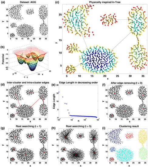
Figure 1.
The idea of the proposed clustering method. (a) A synthetic dataset from literature [39]. (b) An illustration for the potential surface. As the isopotential lines vary from red to blue, the potentials in the corresponding areas become lower and lower. (c) The constructed In-Tree. The colors on nodes denote the potentials corresponding to the cases in (b). (d) The constructed in-tree, in which the inter-cluster edges are colored in red while the intra-cluster edges are in black. Note that the graph structures in (c,d) are the same. (e) The plot in which the lengths of all the edges in the In-Tree are arranged in decreasing order. (f) The result after removing the undesired edges (i.e., the inter-cluster edges). The nodes in red are the root nodes of sub-graphs. (g) The result after the first round of parallel searching of the root node for each non-root node. (h) The results after the last round of parallel searching of the root nodes. All the non-root nodes are directly linked to their root nodes. (i) The clustering result. The samples in the same colors are assigned to the same clusters.
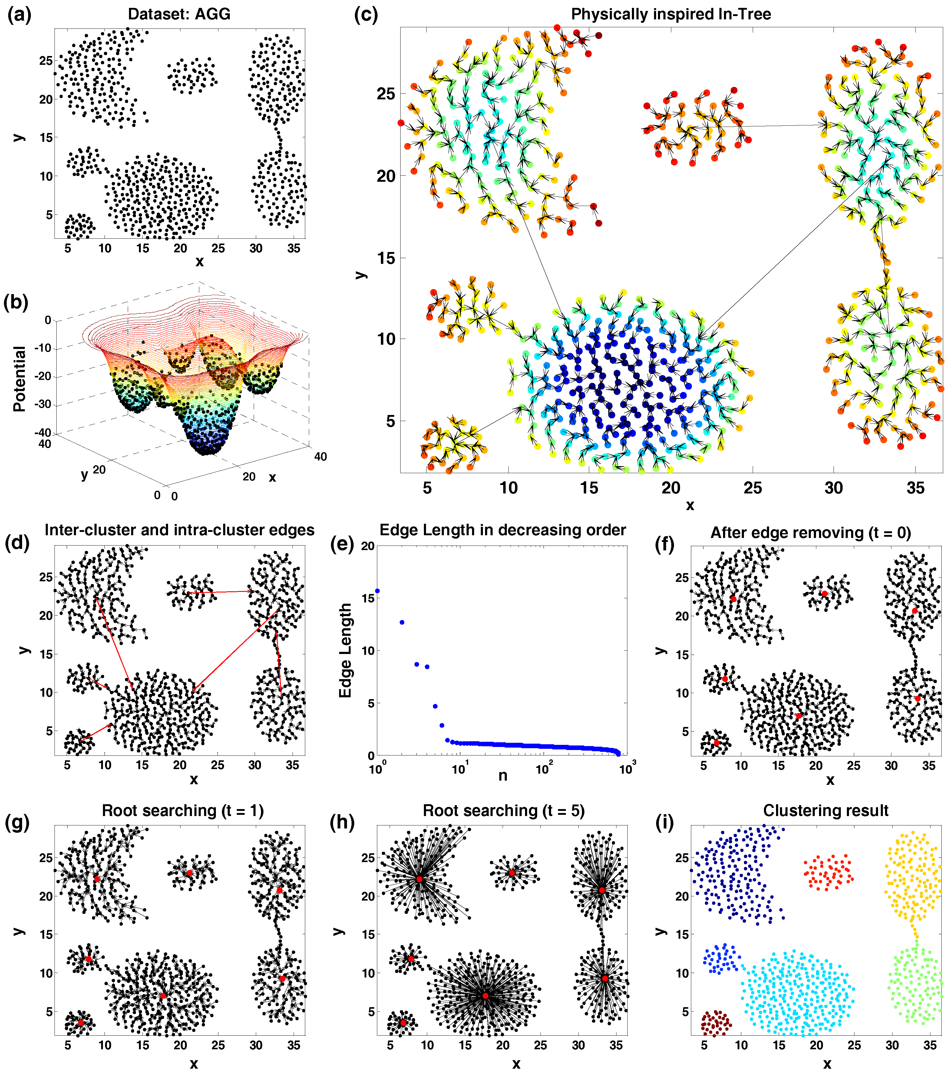
Actually, on this relay-like trajectory, we only need to make effort to determine the first transfer point (also called the parent node) for each point. The reason is that once linking each point to its first transfer point by a directed line (also called the edge), one can obtain an attractive network (or graph), called the In-Tree, in which the discrete data points are efficiently organized (Figure 1c). This In-Tree can then serve as a map, on which the next hops (or the next transfer points) can be easily determined by following the directions of the edges (one can view this graph-based relay based on other points of the group as a sort of Swarm Intelligence).
One problem for this In-Tree is that there exist some inter-cluster edges (i.e., the red edges between clusters in Figure 1d) that require to be removed before conducting the rest steps. Pleasingly, those inter-cluster edges are quite distinguishable; for instance, they are generally much longer than the intra-cluster edges. For this reason, if we define the weight of each directed edge as the distance between its start and end nodes, then we can simply regard the m longest edges as the inter-cluster edges, where m can be determined either based on the pre-specified cluster number or the plot in which all the edge lengths are ranked in decreasing order (Figure 1e). In Section 3.2, we will show other more effective edge-cutting methods. After removing the determined inter-cluster edges, the initial graph will be divided into several sub-graphs (Figure 1f), each containing a special node called the root node (corresponding to the point with the lowest potential of one cluster). Within each sub-graph, all the sample points will reach their root node by successively hopping along the edge directions (Figure 1g,h show two intermediate results). Lastly, the samples that are associated with the same root nodes will be assigned into the same clusters (Figure 1i).
3.2. Basic Implementation
Let be a dataset of N sample points and be the corresponding data indexes. Each point can be either a real-valued or character-typed vector. The proposed method contains 3 stages and 10 steps (stage I: steps 1; stage II: steps : stage III: ), as follows:
- Stage I: make the dataset organized into the In-Tree structure. This stage contains the following steps:
- -
- Step 1, compute the distance between each pair of points :where denotes the distance between sample and (in this paper, the Euclidean distance is used, for which ).
- -
- Step 2, compute the potential at each point :where is a parameter, usually called the kernel bandwidth. It is noteworthy that the magnitude of , i.e., , can be also viewed as the density at node i estimated via the exponential kernel function.
- -
- Step 3, determine all the candidate parent node set of each point :
- -
- Step 4, determine the parent node of each point :
- -
- Step 5, build a directed graph, denoted as , for which the node set and the edge set . In Section 3.3.2, we will demonstrate that is an In-Tree, in which each point i has one and only one directed edge started from it and there is a particular node in , called the root node (denoted as r), for which . Note that (1) the min operation outside the parentheses of Equation (9) serves to guarantee the uniqueness of ; (2) the second term (i.e., ) of serves to select the nodes with smaller indexes among the nodes with same potential as node i. However, if there is no such node with the same potential as node i (this case is very common in practice), is actually determined by .
- Stage II: cut the inter-cluster edges. This stage contains the following steps:
- -
- Step 6, define the edge weight. First, we have the following observation: each edge in is associated with the following three features , , and , where
- *
- denotes the distance between the start and end nodes of (i.e., );
- *
- () denotes the magnitude of the potential at the start node of (accordingly, can be viewed as the density at the start node of );
- *
- denotes the number of points in the circle taking the start point of edge as the center and the distance between the start and end nodes of as the radius.
Since the inter-cluster edges are usually much longer than the intra-cluster edges, the distance could be used as the weight of the edge to determine the inter-cluster edges. However, such -based cutting is quite sensitive to outliers and cluster scales (we will demonstrate this in the experiments). To solve the above problem, we also propose other approaches to define the edge weight. Specifically, the weight of the edge can be also defined as one of the following variables and . - -
- Step 7, determine the inter-cluster edges. After defining the edge weight (by either , , or ), we then regard the edges with the largest edge weights as the inter-cluster edges, where M is the number of clusters. We will compare the above three different edge-weight definition methods in the experiments. Therefore, if the cluster number is pre-defined, the inter-cluster edges can be determined automatically. Otherwise, one can determine the inter-cluster edges interactively following the Decision-Graph-based strategy proposed by Rodriguez and Laio [29]. Specifically, one can represent each directed edge by two features such as and . Then, all the edges can be displayed in a 2D scatter plot (Figure 2a). Since only the inter-cluster edges have large values on both and , they will pop out in the scatter plot and thus can be interactively determined. Actually, similar results can be obtained if replacing by (Figure 2b) or (Figure 2c). Nevertheless, it is noteworthy that, in the experiments, we will not use the Decision-Graph-based cutting method to determine the inter-cluster edges, since sometimes it is hard for users to make a decision when the Decision Graph does not show very clear pop-out points. Instead, we will use the Decision Graph (referring to the 2D scatter plot based on features W and ) to validate the effectiveness of the automatic cutting methods (we will detail this in Section 4).
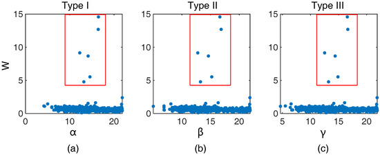 Figure 2. Illustration of different Decision-graph-based methods for determining the inter-cluster edges. (a–c) Different types of scatter-plot-based cutting (Type I: a; Type II: b; Type III: c). The pop-out points within the red rectangles correspond to the inter-cluster edges.
 - -
- Step 8, remove the inter-cluster edges. Assume that are the indexes of the start nodes of the determined inter-cluster edges. Then, the inter-cluster edges are removed by setting (). Each node will become a new root node of the generated graph.
- Stage III: make cluster assignments. This stage contains the following steps:
- -
- Step 9, update the parent nodes. In each round of updating, the parent node of each node i () is updated in this way where denotes the parent node of node i in the t-th round of updating (), and . The updating stops in a certain round when the parent nodes of all nodes no longer change, which means each node is directly linked to its root node (i.e., at this moment, stores the index of the root node that node i reaches), as shown in Figure 1h.
- -
- Step 10, obtain the clustering result (a partition of X). Let , where r is the root node of . The original dataset X is divided into M clusters as follows: , where ().
The pseudocode of the proposed method is shown in Algorithm 1.
| Algorithm 1 ND-C |
| Require:: test dataset; : kernel bandwidth; M: cluster number; |
| Ensure:; // a partition of containing M clusters; |
|
In the following, we also provide an example to illustrate the result of each step of the proposed method on a 1-dimensional dataset as follows: , where , , , , , , and . This dataset can be seen in Figure 3. We set the cluster number and the kernel bandwidth . The main results of each step of the proposed method are listed as follows.

Figure 3.
A 1-dimensional test dataset. Each point represents a 1-dimensional sample.
- Step 1: denotes the ()-entry of the following matrix:
- Step 2:, , , , , , and ;
- Step 3:
- -
- ;
- -
- ;
- -
- ;
- -
- ;
- -
- ;
- -
- ;
- -
- ;
- Step 4:, , , , , , and ;
- Step 5: for ,
- -
- ;
- -
- ;
- -
- .
- Step 6:
- -
- , , , , , and ;
- -
- , , , , , and ;
- -
- , , , , , and ;
- Step 7: ; note that for the test data here, no matter which feature (, , or ) was used to define the weight of each edge , .
- Step 8: , , , , , , and ;
- Step 9: , , , , , , and ;
- Step 10: , , , and .
3.3. Analysis
This section contains the analysis of the two key elements involved in the proposed method, i.e., Nearest Descent (Section 3.3.1) and the In-Tree (Section 3.3.2), as well as the analysis of the time complexity of the proposed method (Section 3.3.3) and the relationship between the proposed method and three most similar methods (Section 3.3.4).
3.3.1. Nearest Descent
The second term in Equation 8 serves to (i) guarantee the uniqueness of the parent node and (ii) avoid the unexpected “singleton cluster phenomenon” in some special circumstances (see details in Appendix B). If we simply define the candidate parent node set as by ignoring the second term in its original definition given by Equation 8, a more explicit understanding is obtained toward the nature of parent node, i.e., for each point, its parent node is the nearest one among the nodes in the descent direction of potential. Furthermore, we name this parent node selection method simply as Nearest Descent (ND) (in contrast to the classical method of Gradient Descent or Steepest Descent), where
- “Nearest” specifies the local choice (or criterion).
- “Descent” specifies the global direction (i.e., in the descending direction of potential), which serves as a constraint to the local choice.
Thus, ND is actually a constrained proximity rule, different from the classical proximity rules such as k-Nearest-Neighbor (k-NN) and -Nearest-Neighbor (-NN) in which the neighbors (or the parent nodes) of any node i are simply defined as the k nearest nodes to node i (i.e., k-NN) and the nodes within a radius centered at node i (i.e., -NN), respectively. Both k-NN and -NN can be viewed as non-constrained proximity criterions. In addition, ND abandons the term Gradient, which makes ND essentially different from the Gradient Descent (GD).
Moreover, since ND regards the samples as nodes in Graph Theory, the proposed clustering method is blind to the underlying features of the samples. Consequently, though inspired from the physical world, ND turns out to be a generalization of the physical world, applicable to the datasets in any high-dimensional space irrespective of whether it is Euclidean space or not. This allows the proposed clustering algorithm to have wide applications.
3.3.2. In-Tree
In Graph Theory [40], as opposed to the Out-Tree, an In-Tree, also called in-arborescence or in-branching, is a digraph that meets the following conditions:
- (a)
- Only one node has outdegree 0;
- (b)
- Any other node has outdegree 1;
- (c)
- There is no cycle in it;
- (d)
- It is a connected graph.
Accordingly, we have the following result (see the proof in Appendix C).
Proposition 1.
The physically inspired graph constructed in Stage I is an In-Tree.
In Figure 4, we compare this physically inspired In-Tree with other popular graphs like the k-nearest-neighbor graph (k-NNG) and Minimal Spanning Tree (MST) on the same dataset. Both k-NNG and MST are widely used in graph-based clustering [41,42,43,44,45,46,47,48,49,50]. From Figure 4, we can see the following two features:

Figure 4.
Comparison between the physically inspired In-Tree (left), k-NNG (middle) and MST (right). Unlike the physically inspired In-Tree whose inter-cluster edges (in red) are relatively longer than the rest inter-cluster edges, both k-NNG and MST contain very short inter-cluster edges (see the local areas circled by the red boxes).
- Like MST and k-NNG, this physically inspired In-Tree follows well the cluster structure in the dataset.
- Although there are some inter-cluster edges in this physically inspired In-Tree, those edges are quite distinguishable, in contrast to the cases in MST and k-NNG.
The 2nd feature makes it possible to easily and reliably determine those inter-cluster edges by diverse methods. The 1st feature guarantees the meaningfulness of the discovered clusters.
Besides the above specialties of this physically inspired In-Tree, the In-Tree graph structure itself has very good properties [40], which facilitate the reliability and efficiency of clustering:
- Removing any edge in the In-Tree will divide the In-Tree into two sub-graphs, each still being an In-Tree.
- There is one and only one directed path between each non-root node and the root node.
The 1st property guarantees that, after removing inter-cluster edges, there will be M sub-graphs and thus the original dataset X will be divided into M non-empty clusters , with ; , .
The 2nd property guarantees that when searching along the directed edges on the generated sub-graphs, each non-root node is sure to reach its root node in the same sub-graph in finite steps. Note that this search on the graph is in essence different from the numerical iteration in the methods such as MeanShift.
3.3.3. Time Complexity
Steps 1∼3 require time. Steps 4∼6 require time. Since step 7 requires to sort the weights of edges, the time complexity of this step is . Step 8 requires time. For step 9, since each time of updating the parent nodes of all the nodes means that the length of path from each leaf node to the reached root node in the previous graph is halved, the time complexity of this step is , where H is the length of the longest path in . The time complexity of step 10 is . Thus, the total time complexity of the proposed method is .
3.3.4. Comparison with Three Similar Clustering Methods
Admittedly, the proposed method is very similar to the following three clustering methods: PHA [27], Quickshift [28], and RL’s method [29]. We briefly introduced these three similar methods in Section 2. Based on the above detailed introduction of the proposed method, here we will make detailed comparison between the proposed method and the above similar methods.
Comparison with PHA. The proposed clustering method is also a potential-based graph-theoretical hierarchical clustering method such that the whole procedure of the proposed method is very similar to that of PHA. However, unlike PHA, (1) we define the potential based on the exponential kernel function (we will show the advantage of this change in the experiments); (2) we give more sophisticated definition for the parent node and we link each node i to its parent node (we also prove that the constructed graph is an in-tree); (3) besides using the Euclidean distance between each node and its parent node to define the edge weight, we also use other more effective ways to define the edges; and (4) we use a scatter-plot-based visualization method to validate the effectiveness of the edge cutting (we will demonstrate its effectiveness in the experiments).
Comparison with QuickShift and RL’s method. The relationship between the proposed method and density clustering (especially QuickShift and RL’s method) is due to the close relationship between the potential and density. Specifically, the magnitude of , i.e., , can be viewed as the density of node i estimated based on the exponential kernel function. In addition can be equivalently written as Accordingly, the parent node selection rule can be viewed as the method of Nearest Ascent in the density perspective; here Nearest Ascent means that each point jumps to the nearest point in the ascending direction of density, or simply speaking, each point ascends to the nearest point. Thus, the proposed method can be viewed as a non-gradient density-peak-based clustering method using Nearest Ascent (NA).
If we let (for both QuickShift and RL’s method), we will find that NA is very similar to QuickShift and RL’s method in terms of parent node definition, as compared in Table 2. Note that for RL’s method, the parent node of each node i is not explicitly defined; the expression of in Table 2 is derived from the definition of in Equation (5). Actually, RL’s method does not explicitly construct a graph, either. However, the density-peak points can be viewed as the start nodes of the inter-cluster edges in the graph constructed by the proposed method. In other words, RL’s method is in the perspective of nodes, while our method and QuickShift are in the perspective of edges. From Table 2, we can see that the difference among QuickShift, RL’s method, and NA on the parent node definition is very small (mainly involving the consideration of some special cases), which has a very limited influence on the ultimate clustering results, as revealed by the experimental results.

Table 2.
Comparison between QuickShift, RL’s method, and NA on the definition for the parent node . , , and .
Compared with QuickShift, the contributions of this paper are as follows:
- We find a more effective feature (i.e., feature ) to define the edge weight such that the proposed method is more insensitive to the data dimension, outlier, and cluster scale.
- We give more sophisticated definition on the parent nodes and strictly prove the constructed graph is an in-tree (rather than a minimal spanning tree).
- We combine the proposed method with RL’s method, using RL’s Decision Graph to validate the effectiveness of each automatic edge cutting method.
Compared with RL’s method, the contributions of this paper are as follows:
- We reveal the nature of the common idea, i.e., Nearest Ascent (from the perspective of density) or Nearest Descent (from the perspective of potential), which helps make a direct connection and significant comparison with the classical ones such as gradient-ascent-based density clustering methods;
- We introduce the graph structure, In-Tree, into the clustering field;
- We present a more general framework (i.e., first estimate the potential, then construct the In-Tree, and lastly remove the inter-cluster edges in the In-Tree), in which RL’s method can be viewed as a scatter-plot-based method to determine the inter-cluster edges.
Actually, a similar clustering idea can be also found in the literature [51], where the clustering method, called Nearest-better clustering, was proposed to enable niching on the multimodal fitness landscapes rather than to solve the general clustering problems. Consequently, the effectiveness of this Nearest-better clustering method is not fully revealed in literature [51] and as a result, it receives little attention. Moreover, the literature [51] claims that the constructed graph is a minimal spanning tree, which is not accurate as revealed Figure 4 by this study.
4. Experiments
First in Section 4.1, we compare three different automatic implementations of the proposed method with other related methods on both synthetic and real-world datasets. Then in Section 4.2, we further compare the three different automatic implementations of the proposed method with regard to the sensitivity to noise, outlier, cluster scales, parameters, and sample order. Additionally, we will also demonstrate the effectiveness of the Decision-Graph-based visualization method for validating the effectiveness of the automatic cutting methods.
4.1. Comparison with Other Methods
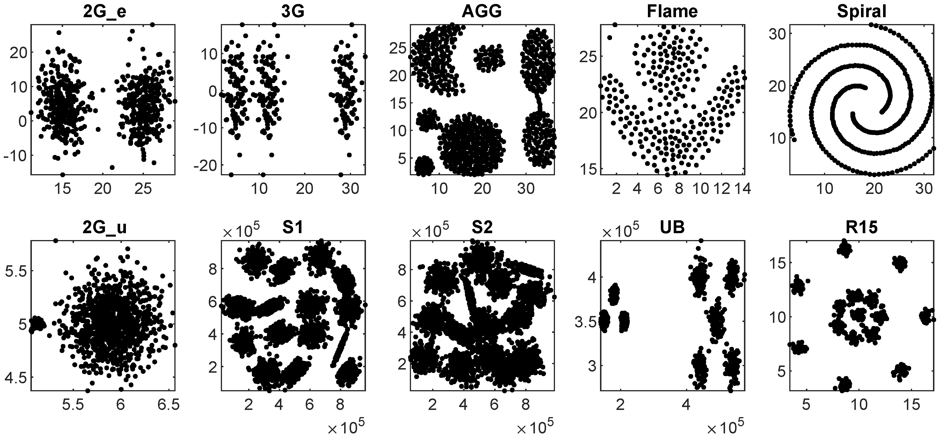
Test datasets. The characteristics of the datasets are shown in Table 3, where the first ten datasets are synthetic datasets (see their cluster structures in Figure 5) while the other eight datasets are real-world ones. For the real-world datasets OrlFace, Coil20, USPS, Pendigits, and Coil100, they does not involve the feature extraction process (i.e., the pixel values of the images were directly used); for the Banknote and Mfeat datasets, more sophisticated features were extracted from the input images [52]. The MetRef dataset was derived from the nuclear magnetic resonance spectra of urine samples [53].

Table 3.
Characteristics of the test datasets. N: number of samples; Dim: number of dimensions; CN: cluster number; TS: this study; RW: Real-world; CV: computer vision.

Figure 5.
Visualization of the 2-dimensional synthetic datasets.
Compared methods. Since the proposed method simultaneously belongs to the categories such as physically-inspired clustering, density-based clustering, and hierarchical clustering, we selected the most relevant methods from these classes. Since the proposed method requires the cluster number as a priori information, all the compared methods can make use of the cluster number as well. What is more, to maximally reduce the influence of the parameter setting, the compared methods either have no parameter or have the suggested empirical settings for the contained parameters. The details of the compared methods are introduced as follows.
- S-Link: Single Linkage hierarchical clustering method [61].
- A-Link: Average Linkage hierarchical clustering method (also called the unweighted pair group method with arithmetic means algorithm) [62].
- PHA: a fast potential-based hierarchical agglomerative clustering method [27]. In the experiments, we used two versions of PHA, denoted as PHA-1 and PHA-2, where
- -
- PHA-1 uses the default potential estimation method of PHA;
- -
- PHA-2 uses the same potential estimation as the proposed method.
- QuickShift: a density-based hierarchical agglomerative clustering method [28]. In the experiments, QuickShift used the same kernel (i.e., an exponential kernel) as the proposed method to estimate the density at each node.
- RL: a density-peak-based clustering method proposed by Rodriguez and Laio [29]. In the experiments, we used two versions of RL, denoted as RL-1 and RL-2, where
- -
- RL-1 uses the default Gaussian kernel to estimate the density;
- -
- RL-2 uses the same kernel function (i.e., the exponential kernel function) as the proposed method to estimate the density.
- DLORE_DP: a recent variant of RL [63].
- ND-C: the proposed method. We used three automatic versions of ND-C, denoted as ND-C(1), ND-C(2), and ND-C(3), which only differ in how they define the edge weight. Specifically,
- -
- For ND-C(1), the distance feature is used to define the weight of each edge in the constructed in-tree;
- -
- For ND-C(2), feature is used to define the weight of each edge in the constructed in-tree;
- -
- For ND-C(3), feature is used to define the weight of each edge in the constructed in-tree;
where , and are the three features associated with each edge in the constructed in-tree; see more details in Section 3.2 (stage II).
Parameter setting. Both S-Link and A-Link do not contain any parameter. Note that, in this study, we do not view the cluster number as a parameter. For all the compared methods, we set the cluster number as the true number of classes of each test dataset. For all the methods that involve the parameters, their default parameter settings were used. Specifically, For PHA-2, QuickShift, RL-1, RL-2, ND-C(1), ND-C(2), and ND-C(3), we fixed the kernel bandwidth to the () percentile of all the pair-wise distances. PHA-1 contains a density-related parameter, which was set by its default setting (). DLORE_DP also contains a parameter, for which we chose its default setting (). Besides, to make the results of the compared methods producible, for RL-1, RL-2, and DLORE_DP, the density-peak points were determined using the automatic methods based on the cluster number and the product (i.e., the defined variable in [29]) of the density and the distance from each node to its parent node.
Evaluation indexes. Two widely used external evaluation indexes were used to evaluate the accuracy of the clustering result, which are the normalized mutual information (NMI) [64] and the adjusted Rand index (ARI) [65]. The value of NMI ranges from 0 to 1, while the value of ARI ranges from −1 to 1. Higher values of NMI and ARI indicate better performance of clustering methods. Note that different evaluation indexes (e.g., NMI and ARI) are defined using different principles (see the definitions of NMI and ARI in Appendix D), which evaluate the clustering accuracy from different aspects.
Results. The NMI and ARI scores of the compared methods are shown in Table 4 and Table 5, respectively, where we can see that ND-C(3) achieves overall the best performance. Specifically,

Table 4.
The NMI scores of different methods on different datasets (the names of synthetic datasets are in italics). The best performance on each dataset is highlighted in bold.

Table 5.
The ARI scores of different methods on different datasets. The best performance on each dataset is highlighted in bold. The names of synthetic datasets are in italics.
- ND-C(1), ND-C(2), and ND-C(3) show the same NMI and ARI scores on all the synthetic datasets (in italics). However, on the real-world datasets (which are high-dimensional datasets), ND-C(1) performs much worse than ND-C(3). However, by taking both distance and potential features into account, ND-C(2) performs overall better than ND-C(1), but it still performs overall worse than ND-C(3).
- Besides ND-C(1) and ND-C(2), ND-C(3) also achieves overall better performance than all the other compared methods.
Furthermore, it is noteworthy that PHA-2, QuickShift and ND-C(1) achieve the same performance on all the datasets (this is also the case for RL-2 and ND-C(2)), which demonstrates again the close relationship between PHA, QuickShift, RL, and the proposed method.
4.2. Further Comparison of ND-C(1), ND-C(2), and ND-C(3) and The Usage of the Visualization Tool for Validation
In the following, we will further compare the three different automatic implementations (i.e., ND-C(1), ND-C(2), and ND-C(3)) of the proposed method with regard to the sensitivity to noise, outlier, cluster scales, parameters, and sample order.
Remark: In step 7 of the proposed method (Section 3.2), besides the automatic cutting methods, we also introduce the Decision-Graph-based interactive methods to determine the inter-cluster edges. In this section, we will not directly validate the effectiveness of the Decision Graph by interactively determining the inter-cluster edges based on it. Instead, we will validate the effectiveness of Decision Graph indirectly by taking it as a visualization tool to reveal the effectiveness of different automatic cutting methods. Specifically, in the Decision Graph, the points will be colored based on whether the corresponding edges are removed by the automatic cutting methods or not. If the edges are removed, the corresponding points in the Decision Diagram are colored in red; otherwise the corresponding points in the Decision Diagram are colored in blue. We call the above Decision Graph with two classes of points the 2-classification Decision Diagram. Note that we use Diagram rather than Graph in the above term in order to distinguish it from the graph concept in graph theory. Similar to the assumption for the density-peak points in [29], the inter-cluster edges in the in-tree are assumed to have large values in both features (i.e., W and ) in the Decision Graph. Thus, the expected 2-classification Decision Diagrams are the ones in which the red points are all the pop-out points. If there are two pop-out points, the pop-out point with higher density is more likely to correspond to the inter-cluster edge. Note that since the 2-classification Decision Graphs based on features W and are almost the same as the 2-classification Decision Graphs based on features W and (or ), we only show the 2-classification Decision Graphs on features W and in the experiments.
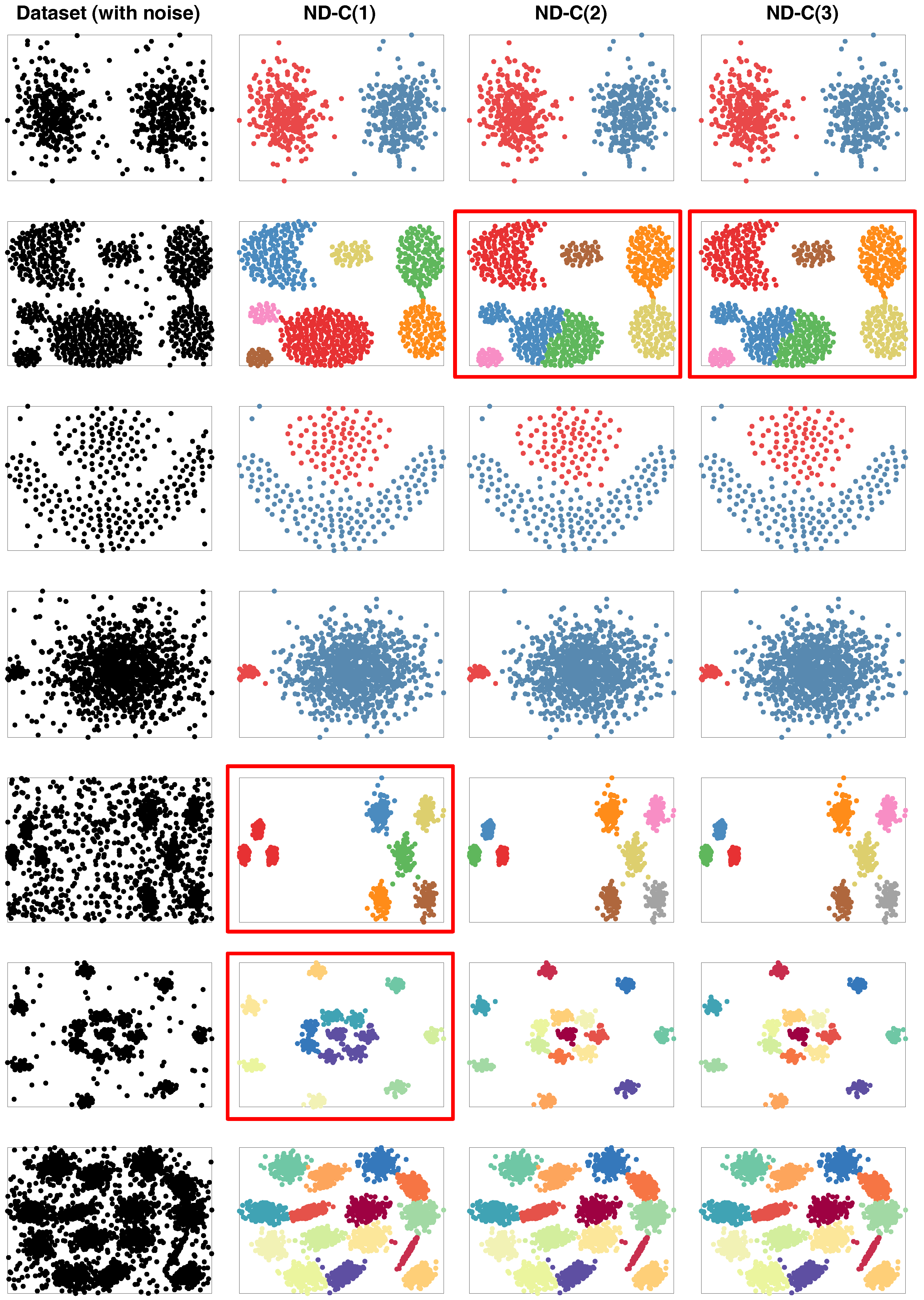
Sensitivity to noise. To study the noise sensitivity of ND-C(1), ND-C(2), and ND-C(3), we added random noise to eight test datasets. For each test dataset, the number of the noise points is 10 percent of the total number of the samples it contains. The first column of Figure 6 shows the datasets with the added noise points. The clustering results of ND-C(1), ND-C(2), and ND-C(3) are shown in the 2nd, 3rd, and 4th columns of Figure 6, respectively; note that for clarity purposes, we removed the noise points in those clustering results and use the red rectangles to mark the failure cases (in each of which there are at least two clusters not separated). The results in Figure 6 show that all of the three implementations are not very sensitive to the the added noise points. Relatively, ND-C(2) and ND-C(3) perform slightly better than ND-C(1). Furthermore, Figure 7 shows the corresponding 2-classification Decision Diagrams of ND-C(1), ND-C(2), and ND-C(3) on all the test noise-contaminated datasets. From the 2-classification Decision Diagrams marked by the red rectangles, we can see that there are some saliently pop-out points (pointed by the red arrows) falsely colored in blue; specifically, since those points pop out in the scatter plots, the corresponding edges are more likely to be the inter-cluster edges, but from their colors, we know that they are not removed by the automatic cutting methods. This explains the underlying reason of the corresponding failure cases in Figure 6. In contrast, for the rest of the 2-classification Decision Diagrams, we can clearly see that all the pop-out points are colored in red (denoting that the corresponding edges are removed).
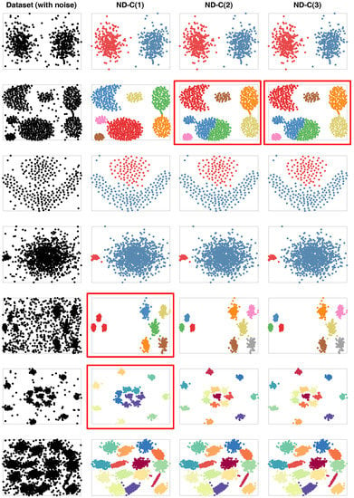
Figure 6.
Comparison of clustering performance of ND-C(1), ND-C(2), and ND-C(3) on noise-contaminated datasets. The subplots within the red rectangles are the ones containing obvious false assignments. In each subplot (in columns 2, 3, and 4), different colors on points indicate different clustering assignments on them.
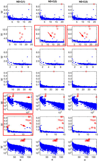
Figure 7.
The 2-classification Decision Diagrams of ND-C(1), ND-C(2), and ND-C(3) on all the noise-contaminated test datasets shown in Figure 6. Each row shows the 2-classification Decision Diagrams of the test dataset shown in the same row of Figure 6. The blue points correspond to the edges that are not automatically removed by the cutting methods; the red points correspond to the edges that are automatically removed by the cutting methods. The red rectangles mark the 2-classification Decision Diagrams with falsely classified points, which are in blue and indicated by the red arrows.
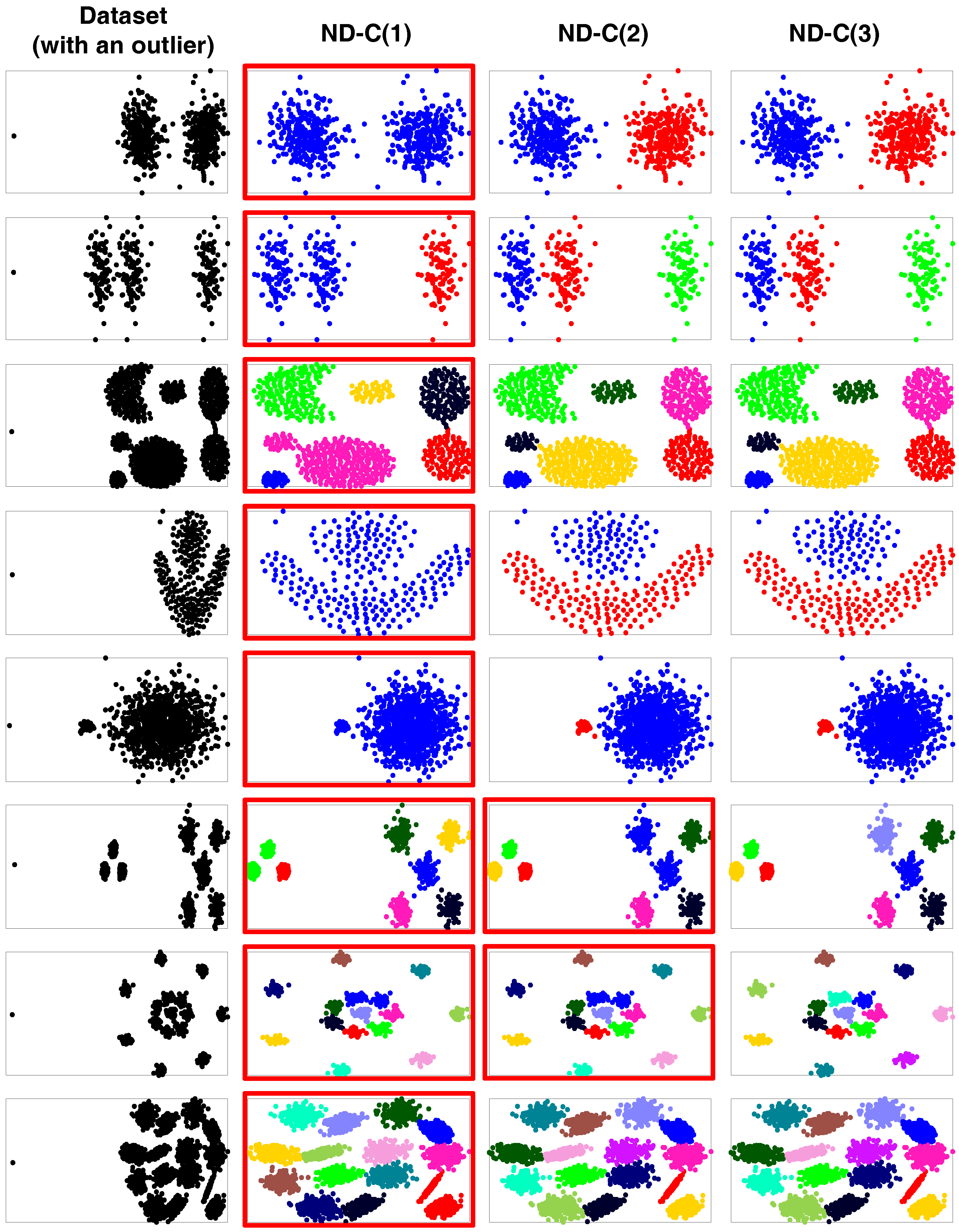
Sensitivity to outliers. To study the outlier sensitivity of ND-C(1), ND-C(2), and ND-C(3), we added an outlier to each selected dataset (i.e., a point that is further apart from the cluster structure). The clustering results are shown in Figure 8, where the 1st column shows the outlier-contaminated test datasets, in each of which the leftmost point is the added outlier. The clustering results of ND-C(1), ND-C(2), and ND-C(3) are shown in the 2nd, 3rd, and 4th columns of Figure 8, respectively; for clarity purposes, we also removed all the outliers in those clustering results and use the red rectangles to mark the problematic results (in each of which there are two major clusters not separated, since the outlier itself is regarded as a singleton cluster). From Figure 8, we can see that ND-C(1) is severely affected by the outliers with all the results being problematic. ND-C(2) performs much better than ND-C(1), but it still contains two problematic results. ND-C(3) performs the best without any problematic result. We also show the 2-classification Decision Diagrams in Figure 9, which shows high consistency with the clustering results in Figure 8. Specifically, for all the problematic clustering results in Figure 8, their corresponding 2-classification Decision Diagrams are also problematic in Figure 9, which are marked by the red rectangles as well, where we also point out the pop-out points that are colored in blue (for those points, the corresponding edges could be the inter-cluster edges but are not removed by the automatic cutting methods).
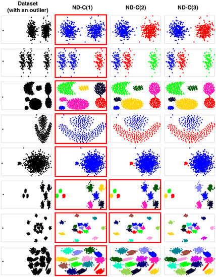
Figure 8.
Comparison of clustering performance of ND-C(1), ND-C(2), and ND-C(3) on the outlier-contaminated datasets. The subplots within the red rectangles are the ones containing obvious false assignments. In each subplot (in columns 2, 3 and 4), different colors on points indicate different clustering assignments on them.
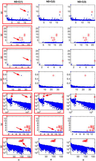
Figure 9.
The 2-classification Decision Diagrams of ND-C(1), ND-C(2), and ND-C(3) on all the outlier-contaminated test datasets shown in Figure 8. Each row shows the 2-classification Decision Diagrams of the test dataset shown in the same row of Figure 8. The blue points correspond to the edges that are not automatically removed by the cutting methods; the red points correspond to the edges that are automatic removed by the cutting methods. The red rectangles marker the 2-classification Decision Diagrams with falsely classified points, which are in blue and pointed by the red arrows.
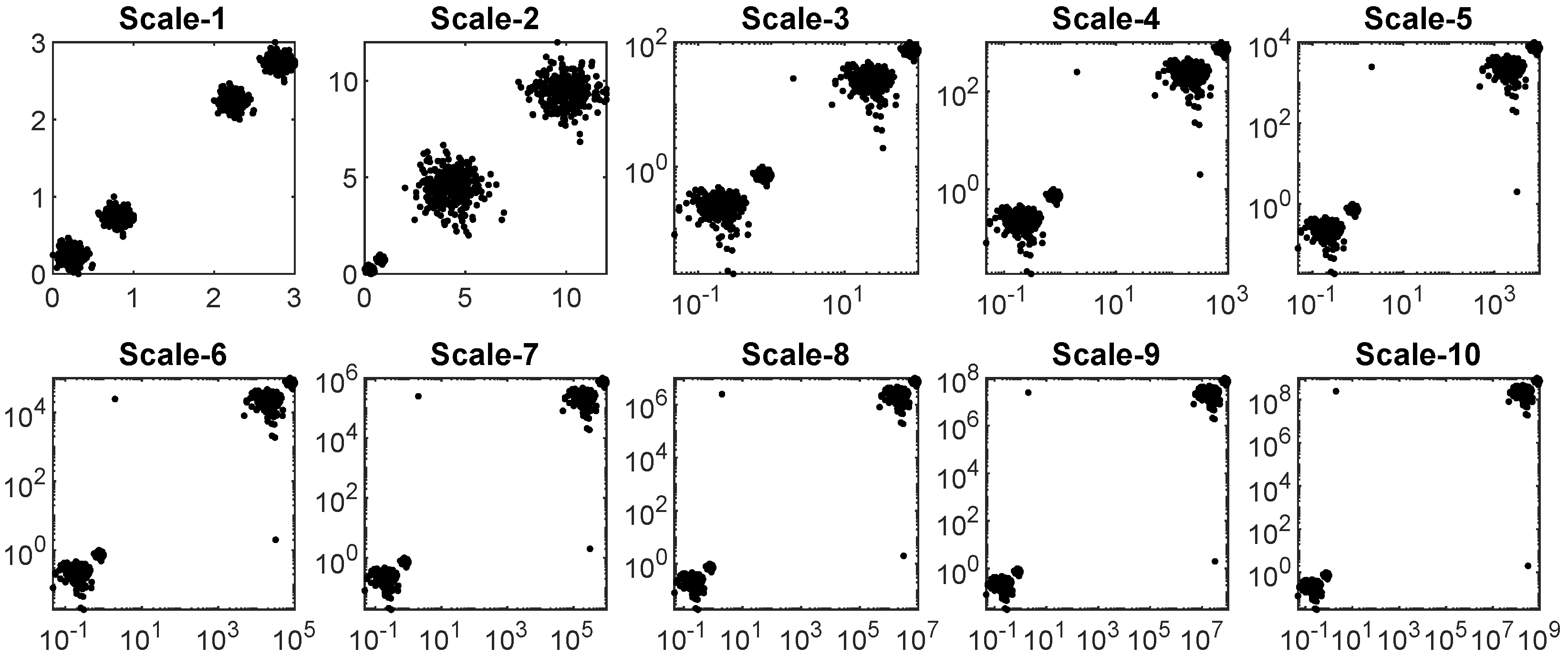
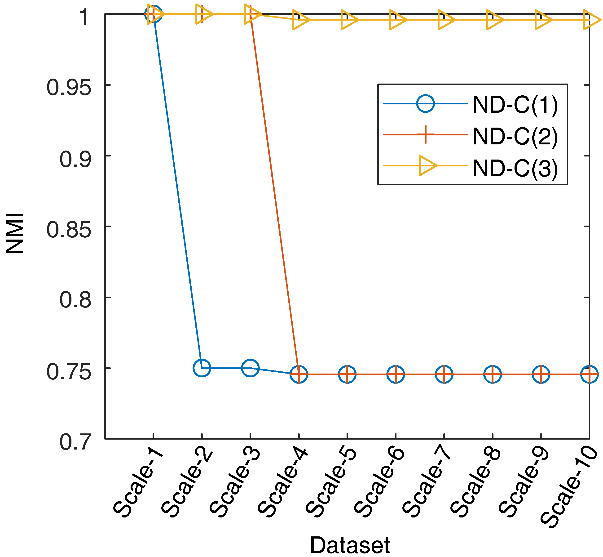
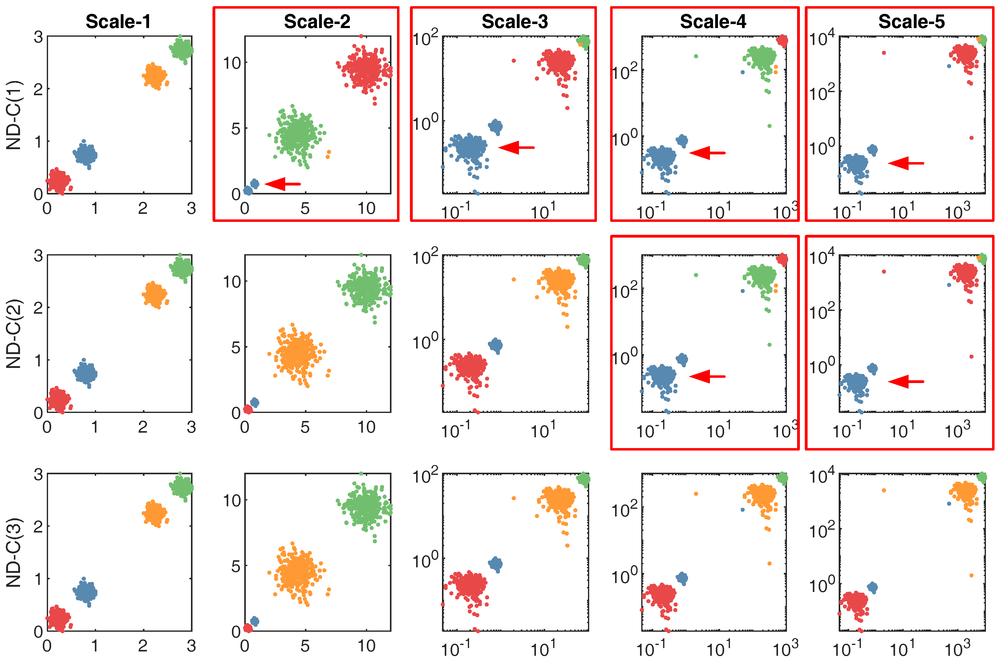
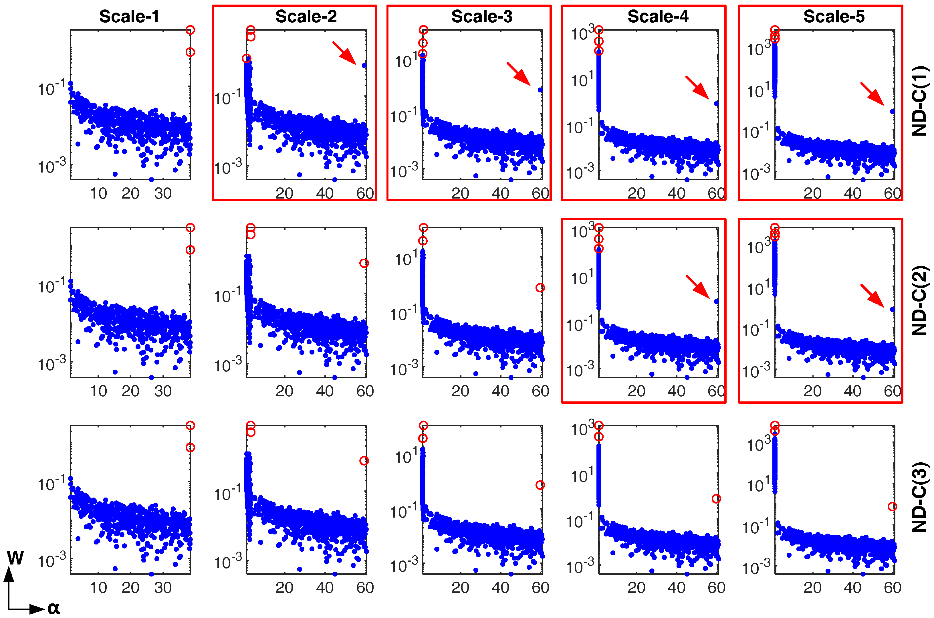
Sensitivity to cluster scale. To study the sensitivity of ND-C(1), ND-C(2), and ND-C(3) to the scale difference of the clusters, we generated ten datasets (named Scale-1, Scale-2,…, Scale-10) with different scales of clusters, as shown in Figure 10. In Figure 11, we compared the NMI scores on those scale-different datasets, where we can see that only ND-C(3) shows almost ideal performance on all the scale-different datasets; this is further demonstrated by the clustering results shown in Figure 12, where only ND-C(3) correctly finds all the clusters in the considered scale-different datasets. The 2-classification Decision Diagrams of ND-C(1), ND-C(2), and ND-C(3) on the first five scale-different datasets also reveal that only ND-C(3) successfully finds all the inter-cluster edges; see Figure 13.

Figure 10.
Ten datasets with different scales of clusters visualized. Except datasets Scale-1 and Scale-2, all the other datasets are visualized in logarithmic scale (in the linear scale, some clusters could not be visually found).
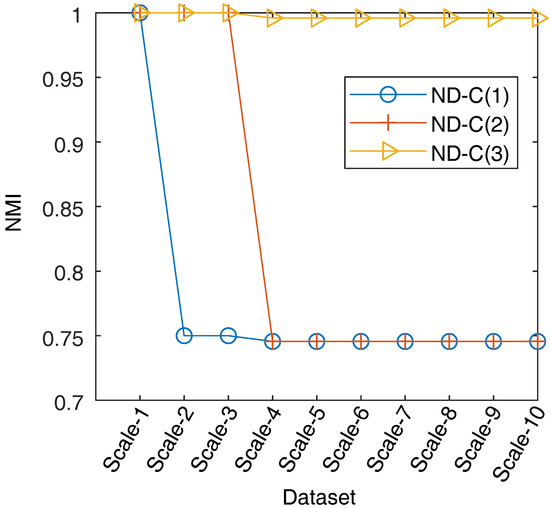
Figure 11.
The NMI scores of ND-C(1), ND-C(2), and ND-C(3) on ten datasets with very different scales of clusters.
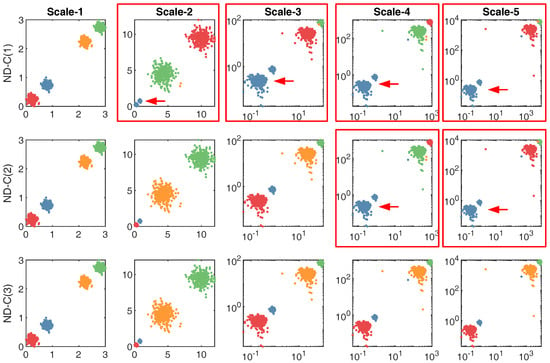
Figure 12.
Comparison of the clustering results of ND-C(1), ND-C(2), and ND-C(3) on the first five scale-different datasets (Scale-1, Scale-2,…, Scale-5) shown in Figure 10. The red rectangles mark the sub-plots with false clustering assignments (pointed by the red arrows).
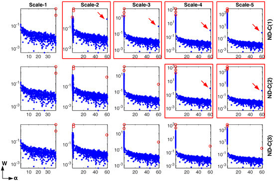
Figure 13.
The 2-classification Decision Diagrams of ND-C(1), ND-C(2), and ND-C(3) on the first five scale-different datasets shown in Figure 10. The red rectangles mark the 2-classification Decision Diagrams with falsely classified points, which are in blue and pointed by the red arrows. For each sub-graph in the first column, there are actually three circles, two of which are overlapped.
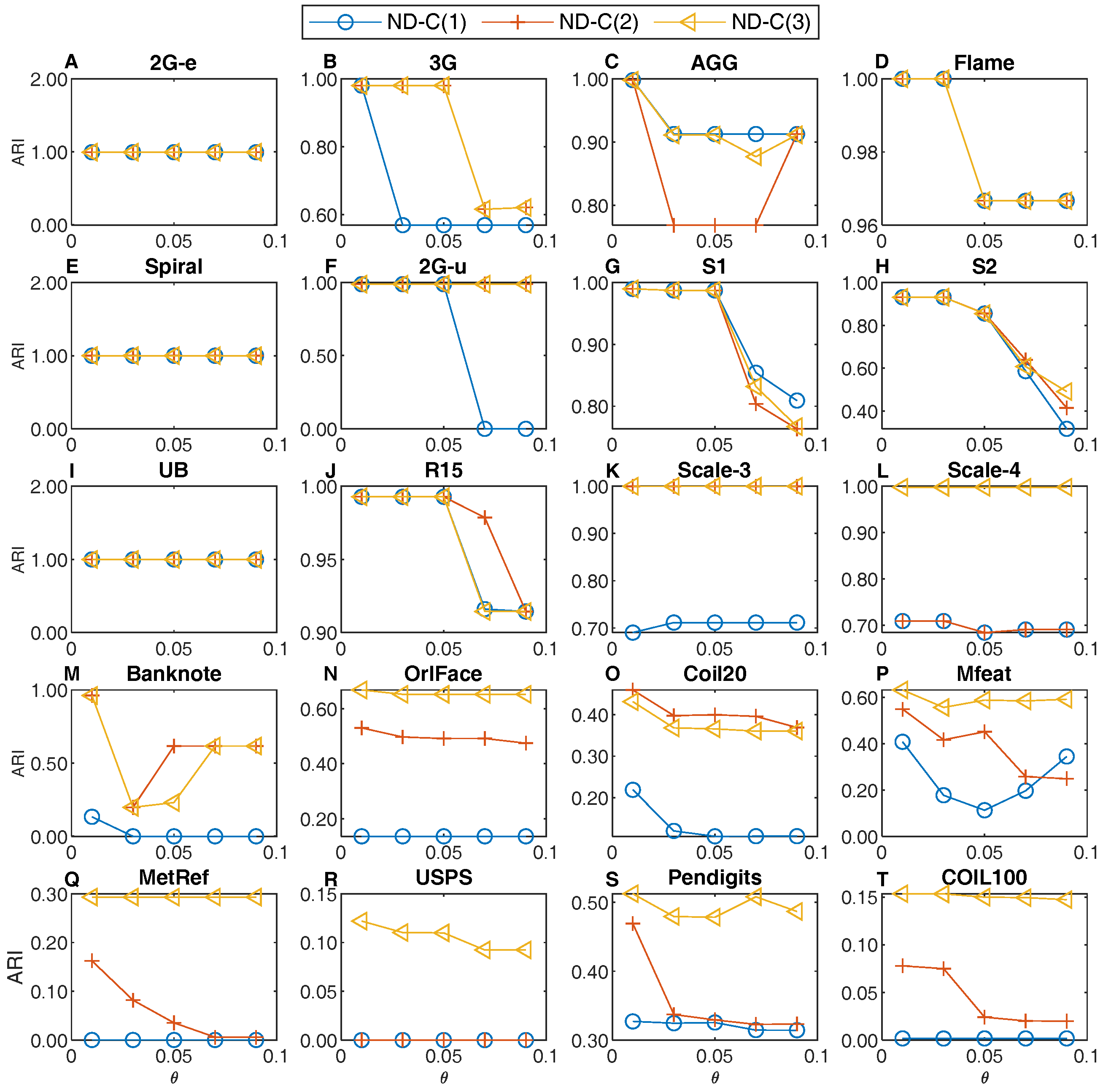
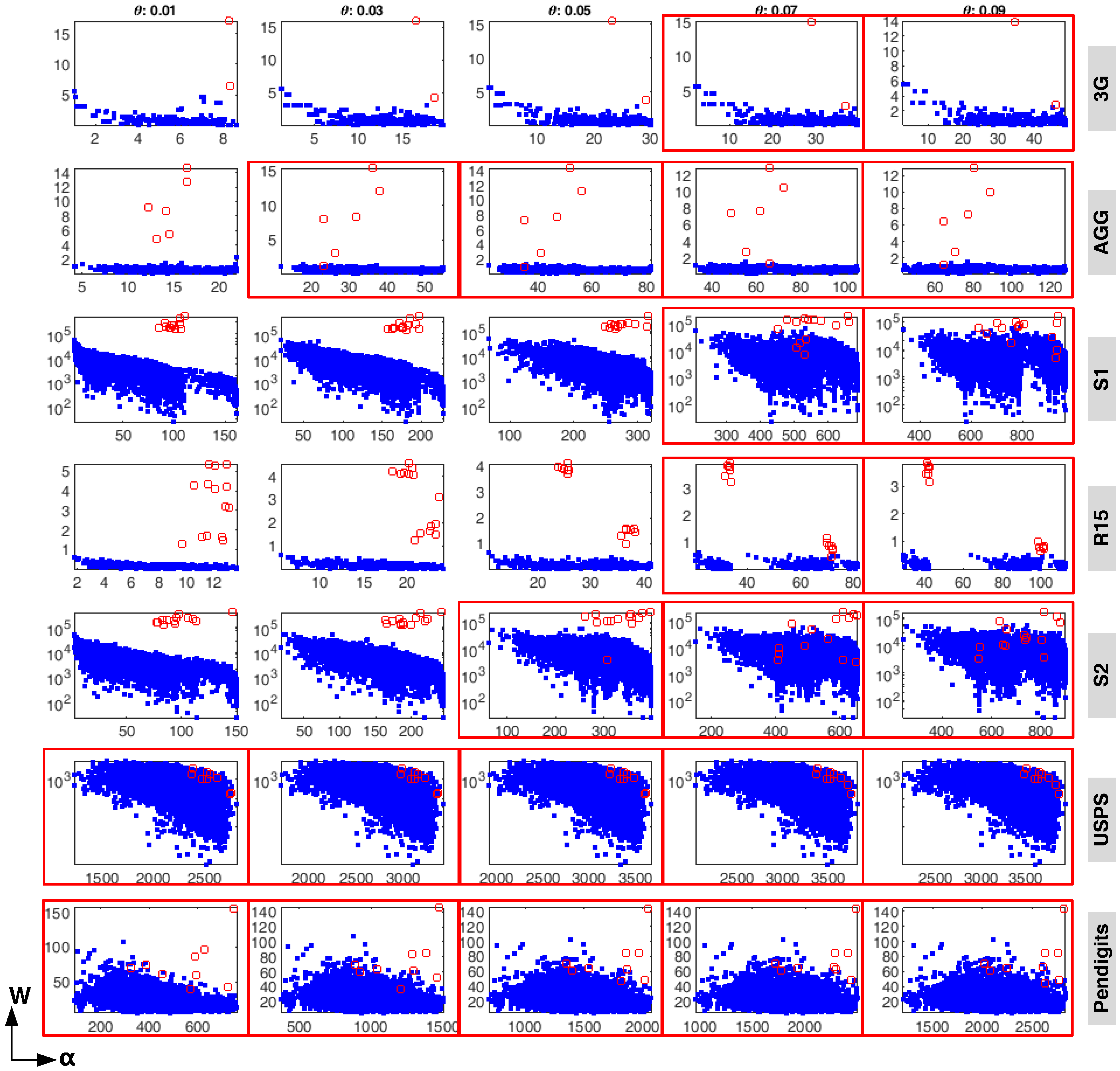
Sensitivity to parameters. To study the parameter sensitivity of ND-C(1), ND-C(2), and ND-C(3), we applied them on twenty datasets with the value of parameter ranging from 0.01 to 0.09 with a step of 0.02. From the ARI scores in Figure 14, we can see that ND-C(1), ND-C(2), and ND-C(3) are overall not very sensitive to the parameter setting, with very robust performance on datasets 2G-e (Figure 14A), Spiral (Figure 14E), UB (Figure 14I), Scale-3 (Figure 14K), Scale-4 (Figure 14L), OrlFace (Figure 14N), Coil20 (Figure 14O), USPS (Figure 14R). Nevertheless, ND-C(3) still performs slightly better than ND-C(1) and ND-C(2); see the results on datasets 2G-u (Figure 14F), Mfeat (Figure 14P), MetRef (Figure 14Q), COIL100 ( Figure 14T). What is more, the values of the ARI scores of ND-C(3) are overall higher than that of ND-C(1), and ND-C(2), especially on the scale-different datasets (see Figure 14 K,L) and most real-world datasets (see Figure 14N,P–T). We also show the 2-classification Decision Diagrams of ND-C(3) with different values of on the seven datasets (3G, AGG, S1, R15, S2, USPS, and Pendigits). The red rectangles in Figure 15 mark the problematic 2-classification Decision Diagrams in which there exist the circles that are not well separated from the blue ones, which are very consistent with the corresponding results in Figure 14 where the corresponding ARI scores are relatively low. Specifically, for the AGG dataset, Figure 14 shows that the ARI score is almost ideal only when . In Figure 15, we can also see that, only in the case of , all the red circles are well separated from the blue points. For USPS, Figure 14 shows that the ARI score is very low in any setting of . In Figure 15, we can also see that in all the 2-classification Decision Diagrams of USPS, the red circles are totally mixed with the blue points, showing the very low reliability of the automatic trimming method on these data. The reason could be that the clusters of this image dataset could lie in the manifold space. Actually, when we embedded USPS dataset to a lower dimension (e.g., 20) by the non-linear dimension reduction method t-SNE [66] and then applied ND-C(3) on it, we obtained much better performance on both the ARI scores and the 2-classification Decision Diagrams, as revealed by Figure 16, where we can also see the consistency of the ARI scores (Figure 16A) and the quality of the 2-classification Decision Diagrams (Figure 16B). Specifically, when and , the red circles in the 2-classification Decision Diagrams are all the pop-out points, and the corresponding ARI scores are also the highest.
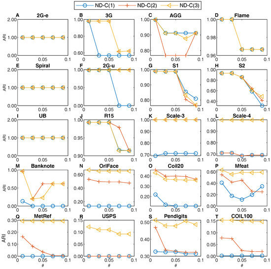
Figure 14.
Comparison of the sensitivity of ND-C(1), ND-C(2), and ND-C(3) to parameter .
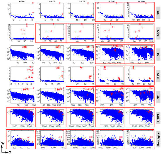
Figure 15.
The 2-classification Decision Diagrams of ND-C(3) with different values of on different datasets. From top to bottom, the test datasets are 3G, AGG, S1, R15, S2, USPS, and Pendigits, respectively. From left to right, the values of of ND-C(3) are 0.01, 0.03, 0.05, 0.07, and 0.09, respectively. The red rectangles mark the 2-classification Decision Diagrams in which there exist the red circles that are not well separated with the blue ones.

Figure 16.
The results of ND-C(3) with different parameter settings on USPS with dimension reduction by t-SNE. (A) the ND scores. (B) the 2-classification Decision Diagrams.
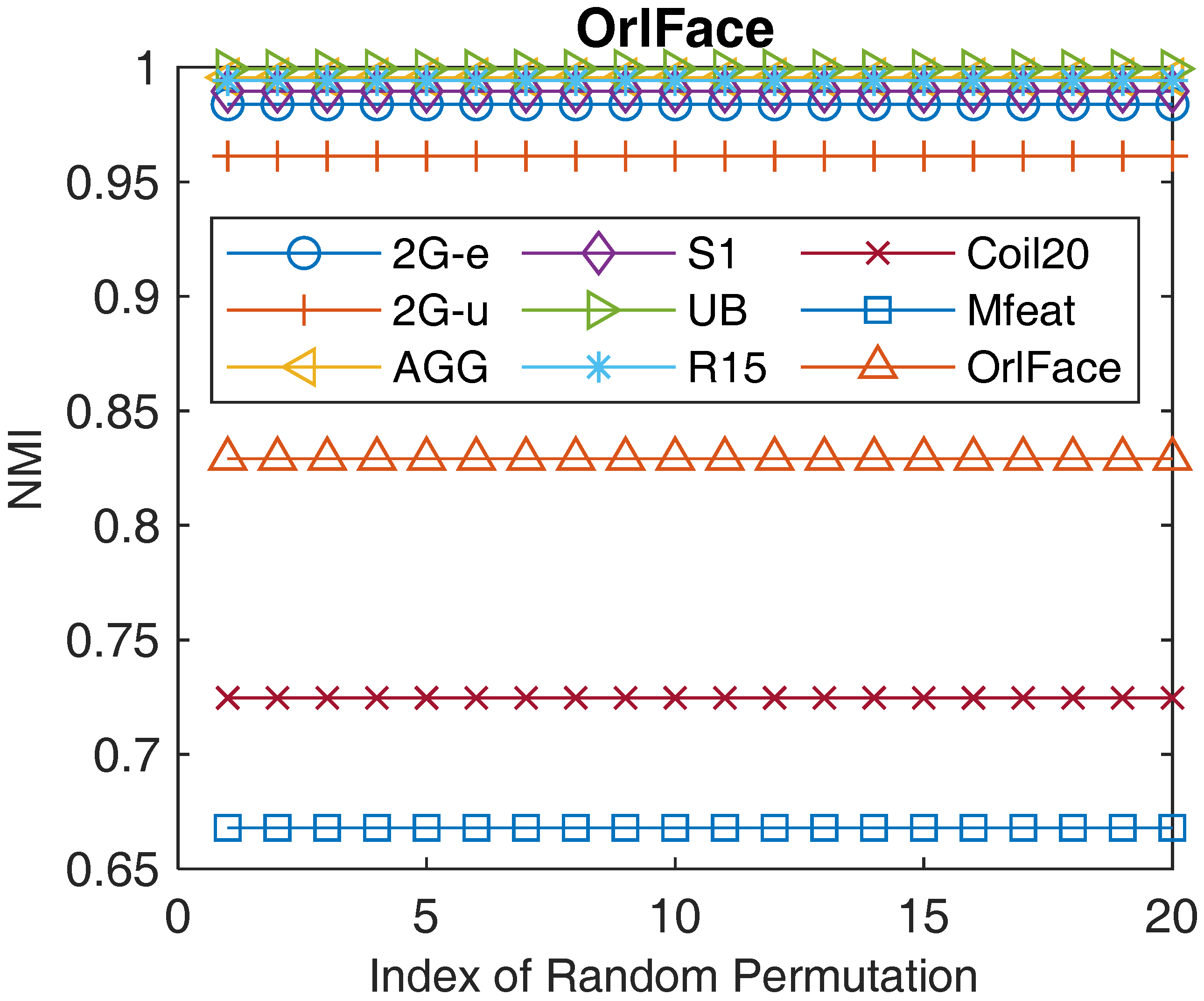
Sensitivity to sample order. To study the sample order sensitivity of ND-C(1), ND-C(2), and ND-C(3), we tested them on nine datasets multiple times. Specifically, we tested each dataset 20 times using each method with the samples randomly permuted each time. The results of ND-C(3) are shown in Figure 17; the results of all the other cutting methods are almost the same as that of ND-C(3) and thus omitted here. These experimental results reveal that ND-C(1), ND-C(2), and ND-C(3) are not very sensitive to the sample order. We also give a detailed analysis for the underlying reason in Appendix B.
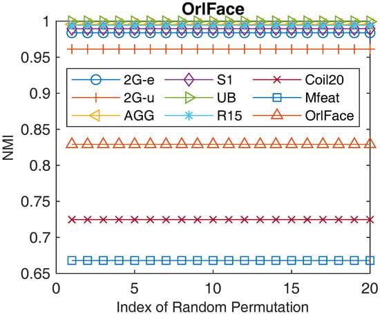
Figure 17.
The NMI scores of ND-C(3) on nine datasets. For each dataset, we applied ND-C(3) on it 20 times and each time we randomly permuted the orders of the samples in the dataset.
5. Conclusions
In this study, we propose a physically inspired graph-theoretical density-based hierarchical clustering method, using a non-gradient paradigm (i.e., Nearest Descent) and a particular digraph (i.e., In-Tree). We demonstrate its effectiveness on both synthetic and real-world datasets. We reveal the connection and difference between the proposed method and the similar methods via both theoretical analysis and experiments. Experimental results also reveal that all the three automatic implementations of the proposed method are not very sensitive to the noise and sample order. Nevertheless, feature proves overall more effective than the feature W and feature to determine the inter-cluster edges especially when handling the high-dimensional datasets, the outlier-contaminated datasets, and the datasets containing different scales of clusters. The experimental results also reveal the meaningfulness of the visualization strategy in increasing the reliability of the clustering results in practice [67].
6. Future Work
In the future, we would like to apply the proposed method to handle more real-world datasets generated in different fields. Additionally, since the proposed method has time complexity, which means that the proposed method would be efficient to handle the medium-size datasets (e.g., the datasets containing tens of thousands of samples), but would not be very efficient when handling the large-size datasets (e.g.,the datasets containing millions of samples). Thus, next, we would also like to accelerate the proposed method using more efficient algorithms in order to efficiently handle the datasets with very large sizes.
Author Contributions
Conceptualization, T.Q. and Y.L.; methodology, T.Q. and Y.L.; software, T.Q.; validation, T.Q. and Y.L.; investigation, T.Q. and Y.L.; data curation, T.Q.; writing—original draft preparation, T.Q.; writing—review and editing, Y.L.; visualization, T.Q.; supervision, Y.L.; funding acquisition, Y.L. All authors have read and agreed to the published version of the manuscript.
Funding
This research was funded by Guangdong Key R&D Research Project (2018B030338001).
Institutional Review Board Statement
Not applicable.
Informed Consent Statement
Not applicable.
Data Availability Statement
The code and data of this study can be found at the following links: https://github.com/Teng-Qiu-Clustering/Nearest-Descent-in-tree-and-Clustering-2022-Mathematics and https://codeocean.com/capsule/2873687/tree/v1 (accessed on 3 February 2022).
Acknowledgments
The authors would like to thank Fu-ya Luo, Cheng Chen, and Nancy Westanmo-Head for revising this paper. The authors would also like to thank Hongmei Yan, Kaifu Yang, Ke Chen, Yezhou Wang and Shaobing Gao for the suggestions.
Conflicts of Interest
The authors declare no conflict of interest.
Abbreviations
The following abbreviations are used in this manuscript:
| ND | Nearest Descent |
| NA | Nearest Ascent |
| ND-C | Nearest Descent based Clustering |
| HC | Hierarchical clustering |
| CSPV | Clustering by Sorting Potential Values |
| PHA | Potential-based Hierarchical Agglomerative |
| GA-C | Hradient-Ascent-based Clustering |
| GGA | Graph-theoretical-based Gradient Ascent |
| RL | Rodriguez and Laio |
| GD | Gradient Descent |
| MST | Minimal Spanning Tree |
| k-NNG | k-Nearest-Neighbor Graph |
| S-Link | Single Linkage hierarchical clustering |
| A-Link | Average Linkage hierarchical clustering |
| NMI | Normalized Mutual Information |
| ARI | Adjusted Rand Index |
| Dim | Dimensions |
| CN | Cluster Number |
| CV | Compute Vision |
Appendix A. Density-Border-Based Clustering
This category (the density-border-based) can be traced back to the work of Hartigan in 1975 [68], while the most popular and widely used algorithm is the one called DBSCAN proposed in 1996 [14]. DBSCAN implicitly defines the density at each data point i as the number of the r-neighboring points of point i within the radius centered at point i, and accordingly defines the points with densities beyond a pre-defined density threshold () as the core points. Here we say that point j is a r-neighboring point of i if point j is within the radius r centered at point i (note that this r-neighborhood relationship is symmetric. i.e., point i is also a r-neighboring point of point j with respect to r). For the non-core points (with densities below ), they are further divided into two parts: the border points and noise points, which differs in that the border points are the neighboring points of certain core points. A cluster is then defined as a maximum set (denoted of ) of core points in which any core point is the r-neighboring or transitively r-neighboring point of any other core point in this set, plus a maximal set (denoted as ) of the border objects which are the neighboring nodes of certain core objects in . Here we say that point j is a transitively r-neighboring point of i if there is a chain of points (where and ) such that and (for any ) are the r-neighboring points to each other. Obviously, this transitively neighboring relationship is also symmetric. DBSCAN has two major problems: (i) the two parameters, r and , are hard to set; (ii) Using a global density threshold , DBSCAN could fail to detect the clusters with varying densities [20,21,22].
Among the various variants of DBSCAN (see a review in [22]), OPTICS [69] and HDBSCAN [70] are more representative.
Unlike DBSCAN which directly seeks for a flat partitioning of the dataset, clustering based on OPTICS (or OPTICS for short) belongs to HC, which divides the clustering process into two distinguishable phases. In the 1st phase of HC, OPTICS first seeks for an effective linear arrangement of the samples in the dataset, via a walk on a minimal spanning tree based on the so-called reachability distances [22]. Then, similar to the Decision Graph [29], OPTICS represents each data point by two variables, its index in the new order and its smallest reachability distance, and then shows the original dataset in a 2D bar plot, called the reachabiltiy plot (each valley in the reachability plot represents a optimal cluster). Actually, there is a close relationship between this reachability plot and the Dendrogram [71]. In the 2nd phase of HC, like Dendrogram, one can obtain a flat clustering result from the reachability plot by such as setting a global threshold (for the parameter r). Compared with DBSCAN, the advantages of OPTICS are threefold. (i) OPTICS is relatively insensitive to the two parameters, r and , especially for r which is usually set as infinity (in the first phase of HC). (ii) By choosing different distance thresholds in the reachability plot (for the parameter r, it is usually set as infinity in the first phase so as to output a complete hierarchical data representation, and is set as a specific threshold in the 2nd phase so as to obtain an optimal flat partitioning of the original dataset), one can easily get all the flat clustering results obtained by DBSCAN* with same values for and r (note that DBSCAN and DBSCAN* differ in that the latter one only takes the core points as the elements of a cluster). (iii) OPTICS can discover the clusters in varying densities that DBSCAN cannot. The underlying reason is that in the 2nd phase one can choose other flexible methods [71] to detect the clusters in more complicated reachability plots in which simply setting a global threshold would fail. Furthermore, OPTICS also benefits another significant variant of DBSCAN, called HDBSCAN [70] (also a HC method).
HDBSCAN [70] was proposed recently in 2015, which follows the two phases utilized in OPTICS. However, compared with OPTICS, HDBSCAN presents a more concise and comprehensible procedure in the 1st phase to make the dataset organized into a condensed Dendrogram based on the concepts such as the minimum cluster size and cluster shrink. In the 2nd phase, HDBSCAN proposes an effective automatic cutting method to extract the flat partitioning result from the condensed Dendrogram. The cutting method is mainly based on the concept of cluster stability and the objective that the sum of the stabilities of the extracted clusters should be the maximal. Theoretically, this automatic cutting method could extract the clusters in varying densities. Compared with OPTICS, HDBSCAN completely abandons the parameter r, and like OPTICS, HDBSCAN is not sensitive to the parameter (the only parameter in HDBSCAN). However, this is at the cost of a time complexity of (corresponding to the worst case of OPTICS when r is set as infinity) [72].
Appendix B. About the Data Index
In the original formula of Nearest Descent (see step 4 of stage I), the data indexes (i.e., the order in which data points are processed), together with the potential values, serve to provide references for parent node selection. The role of the data indexes is to deal with the special case that the close points (or the extreme case, the overlapping ones) could have the same potential. Specifically, the data index term could help the proposed method to choose only one point from those close points to communicate with other points with lower potentials, which can avoid the unexpected “singleton cluster phenomenon” after edge cutting.
However, introducing data index term does not mean that the clustering result is sensitive to the change of data indexes. The influence is very limited, as demonstrated by the experimental results in Section 4.2. The undelying reason is analyzed as follows:
If point i is not with the local minimal potential, then since its candidate point set consists of two groups of points, i.e., the points with smaller potentials (group A) and the points with the same potential but smaller data indexes (group B), only points in group B are affected by data index. The points in group B are so special that they do not always exist. Even if group B is non-empty, according to the “constrained proximity criterion" claiming that only the nearest point or the point with the smallest index among the nearest ones in will be selected as the parent node, the selected parent node is at least very close to point i. Therefore, the change of the data indexes only affects the connections or edges in local areas, whereas these local edges, even they are changed, are in general much shorter than those inter-cluster edges among groups and thus less likely to be cut off. Consequently, the near points connected by these local edges can be clustered into the same groups.
Otherwise, the candidate points with lower potential values in set will come from other groups. So, no matter how data indexes are assigned to those points, the edge between point i and its parent node will in general be much longer than the edges among points within group, and thus will be cut off later. This is what we expect. Consequently, the clustering result will not be largely affected. The above analysis is further demonstrated by a test with different random permutations to dataset “S1”, as shown in Figure A1.
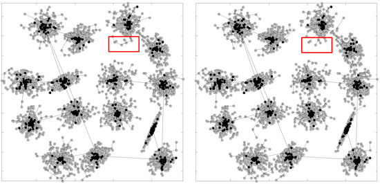
Figure A1.
The experiment for showing the negligible influence of data index. Take dataset “S1” for instance. In order to show the effect of data index, we first generated lots of vertices with identical potentials, since only for these vertices, their data index may serve as a reference for identifying parent nodes. We set as 10, much less than the average pair-wise distance. Consequently, only 151 potential values are unique, which means that most vertices have the same potentials. We randomly changed the data index for 50 times, and the In-Trees of two of the 50 runs are shown in this figure. It is clear that for the edge points in the red rectangles, local difference occurs in their neighborhood relationships, whereas this difference makes very little effect on the final clustering results. In fact, (i) for the in-trees of all 50 tests, we found that the longest 100 edges are the same; (ii) for the clustering results of all 50 tests, when we took one (e.g., the first clustering result) as the benchmark and compared it with the other 49 clustering results, relative clustering error rate were very small, 0.0074 ± 0.0041 (mean ± standard deviation), which means that on average, 37 points out of 5000 get different assignments. To summarize, although the nearest descent rule involves data index item, the change of the data indexes makes negligible influence on the final clustering result.
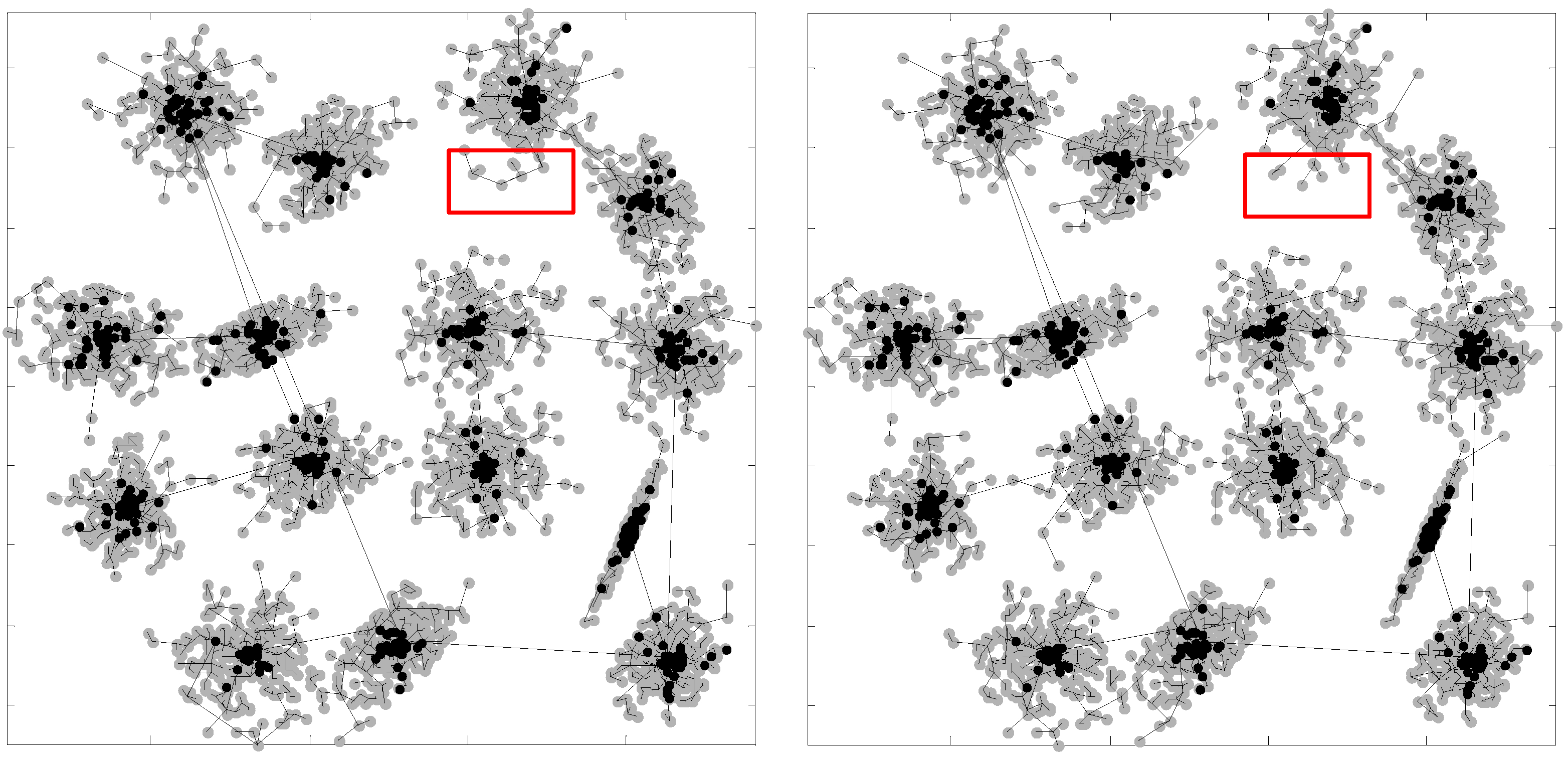
Appendix C. Proof of the In-Tree
Let , , and denote the degree, indegree and outdegree of a node v, respectively. Let G denote any graph. Before proving, we first give the following properties on G [40,73].
- (P1)
- If G is a cycle, then, for any node , = 2. Typically, when the cycle is a directed cycle, .
- (P2)
- If G is a tree, then , where and denote the number of edges and the number of nodes, respectively.
- (P3)
- If G is a digraph, then , and.
Proof of Proposition 1.
First, according to the definition of the graph , we have the following facts:
- (F1)
- For each node i in , () is defined as the points with smaller potentials or the same potential but smaller data indexes;
- (F2)
- For each node i in with , its parent node is unique, i.e., ;
- (F3)
- For each node i in with , it has no parent node, i.e., .
The following proof is then made by showing how the requirements (F1∼F3) can meet the definitions (a∼d) of the In-Tree in Section 3.3.2 of the main body of this paper.
- (i)
- Let be the globally minimal potential among the potentials at all nodes, i.e., . According to; F1, for each node i with , . If only one node i has the minimum potential value, then, according to F1, . If several nodes are of the minimum potential, the node with the smallest index among the above nodes has empty . In conclusion, there is always one and only one node, denoted as r, with , for which, according to F3, . The condition (a) is met.
- (ii)
- According to F1, for any other node , there will be at least one node (e.g., node r) which makes . Then, according to F2, we have . The condition (b) is met.
- (iii)
- Suppose there is a cycle in digraph . If is a directed cycle , then according to F1, the potential values for these nodes should meet , which is true only when . Then according to F1 again, the data indexes for these nodes should meet , resulting in , an obvious contradiction. If is not a directed cycle, we claim that there exists at least one node of , say w, then, according to P1, there will be either or in this cycle . If , then it will contradict with the result in (ii); If , since every node v on a cycle has degree 2, i.e., , and according to P3,there must be at least one node in having outdegree 2, which contradicts the result in (ii) again. Therefore, there is no cycle in digraph . The condition (c) is met.
- (iv)
- Suppose is not connected, e.g., containing T connected sub-graphs , , ⋯, . Since digraph has no cycle, there should be no cycle in each subgraph as well. Hence, each subgraph is at least a tree. Assume the node r of outdegree 0 is in , then nodes in any other subgraph are all with outdegree 1, thus, according to P3,which contradicts P2. Therefore, the digraph is connected. The condition (d) is met.
According to (i), (ii), (iii) and (iv), we can conclude that the digraph is an In-Tree.
Appendix D. NMI and ARI
Let and be the two partitions of the dataset , which means that and (,); and (,). Note that () and () denote two clusters, and that in the experiments, or denotes the partition of determined by the proposed method or determined based on the class labels provided by the benchmark dataset. Then, we have the following definitions of NMI and ARI (note that NMI is a measure based on information theory, while ARI is a measure based on pair counting. Consequently, on certain dataset, a clustering method may show very good performance on one index rather than on all indexes).
(1) The NMI scores between and is defined as
where () denotes the mutual information between and , () denotes the entropy with regard to , and denotes the entropy with regard to . Note that .
(2) The ARI score between and is defined as
where , , and and is the binomial coefficient (). Note that .
References
- Jain, A.K. Data clustering: 50 years beyond K-means. Pattern Recognit. Lett. 2010, 31, 651–666. [Google Scholar] [CrossRef]
- Xu, R.; Wunsch, D. Survey of clustering algorithms. IEEE Trans. Neural Netw. 2005, 16, 645–678. [Google Scholar] [CrossRef] [PubMed] [Green Version]
- Theodoridis, S.; Koutroumbas, K. Pattern Recognition, 4th ed.; Elsevier: Amsterdam, The Netherlands, 2009. [Google Scholar]
- Handl, J.; Knowles, J.; Kell, D.B. Computational cluster validation in post-genomic data analysis. Bioinformatics 2005, 21, 3201–3212. [Google Scholar] [CrossRef] [PubMed] [Green Version]
- Macqueen, J. Some Methods for Classification and Analysis of Multivariate Observations. In Proceedings of the 5th Berkeley Symposium on Mathematical Statistics and Probability; University of California Press: Berkeley, CA, USA, 1967; pp. 281–297. [Google Scholar]
- Frey, B.J.; Dueck, D. Clustering by passing messages between data points. Science 2007, 315, 972–976. [Google Scholar] [CrossRef] [PubMed] [Green Version]
- Eisen, M.B.; Spellman, P.T.; Brown, P.O.; Botstein, D. Cluster analysis and display of genome-wide expression patterns. Proc. Natl. Acad. Sci. USA 1998, 95, 14863–14868. [Google Scholar] [CrossRef] [Green Version]
- McLachlan, G.; Peel, D. Finite Mixture Models: Wiley Series in Probability and Mathematical Statistics; John Wiley & Sons: New York, NY, USA, 2000. [Google Scholar]
- Shi, J.; Malik, J. Normalized cuts and image segmentation. IEEE Trans. Pattern Anal. Mach. Intell. 2000, 22, 888–905. [Google Scholar]
- Ng, A.Y.; Jordan, M.I.; Weiss, Y. On Spectral Clustering: Analysis and an algorithm. Proc. Adv. Neural Inf. Process. Syst. 2002, 14, 849–856. [Google Scholar]
- Cheng, Y. Mean shift, mode seeking, and clustering. IEEE Trans. Pattern Anal. Mach. Intell. 1995, 17, 790–799. [Google Scholar] [CrossRef] [Green Version]
- Comaniciu, D.; Meer, P. Mean shift: A robust approach toward feature space analysis. IEEE Trans. Pattern Anal. Mach. Intell. 2002, 24, 603–619. [Google Scholar] [CrossRef] [Green Version]
- Fukunaga, K.; Hostetler, L. The estimation of the gradient of a density function, with applications in pattern recognition. IEEE Trans. Inf. Theory 1975, 21, 32–40. [Google Scholar] [CrossRef] [Green Version]
- Ester, M.; Kriegel, H.P.; Sander, J.; Xu, X. A density-based algorithm for discovering clusters in large spatial databases with noise. In Proceedings of the 2nd ACM International Conference Knowledge Discovery and Data Mining; AAAI Press: Portland, OR, USA, 1996; Volume 96, pp. 226–231. [Google Scholar]
- Lin, F.; Cohen, W.W. Power iteration clustering. In Proceedings of the 27th International Conference Machine Learning, Haifa, Israel, 21–24 June 2010; pp. 655–662. [Google Scholar]
- Carreira-Perpinan, M.A. Acceleration strategies for Gaussian mean-shift image segmentation. In Proceedings of the Conference Computer Vision and Pattern Recognition, New York, NY, USA, 17–22 June 2006; pp. 1160–1167. [Google Scholar]
- Elgammal, A.; Duraiswami, R.; Davis, L.S. Efficient kernel density estimation using the fast gauss transform with applications to color modeling and tracking. IEEE Trans. Pattern Anal. Mach. Intell. 2003, 25, 1499–1504. [Google Scholar] [CrossRef]
- Georgescu, B.; Shimshoni, I.; Meer, P. Mean shift based clustering in high dimensions: A texture classification example. In Proceedings of the 9th IEEE International Conference Computer Vision, Los Alamitos, CA, USA, 13–16 October 2003; pp. 456–463. [Google Scholar]
- Paris, S.; Durand, F. A topological approach to hierarchical segmentation using mean shift. In Proceedings of the IEEE Conference Computer Vision and Pattern Recognition, Minneapolis, MA, USA, 18–23 June 2007; pp. 1–8. [Google Scholar]
- Ertöz, L.; Steinbach, M.; Kumar, V. Finding clusters of different sizes, shapes, and densities in noisy, high dimensional data. In Proceedings of the 3rd SIAM International Conference Data Mining, San Francisco, CA, USA, 1–3 May 2003; pp. 47–58. [Google Scholar]
- Pei, T.; Jasra, A.; Hand, D.J.; Zhu, A.X.; Zhou, C. DECODE: A new method for discovering clusters of different densities in spatial data. Data Min. Knowl. Discov. 2009, 18, 337–369. [Google Scholar] [CrossRef]
- Kriegel, H.P.; Kröger, P.; Sander, J.; Zimek, A. Density-based clustering. Wiley Interdiscip. Rev. Data Min. Knowl. Discov. 2011, 1, 231–240. [Google Scholar] [CrossRef]
- Kundu, S. Gravitational clustering: A new approach based on the spatial distribution of the points. Pattern Recognit. 1999, 32, 1149–1160. [Google Scholar] [CrossRef]
- Gomez, J.; Dasgupta, D.; Nasraoui, O. A new gravitational clustering algorithm. In Proceedings of the 3rd SIAM International Conference Data Mining, San Francisco, CA, USA, 1–3 May 2003; pp. 83–94. [Google Scholar]
- Sanchez, M.A.; Castillo, O.; Castro, J.R.; Melin, P. Fuzzy granular gravitational clustering algorithm for multivariate data. Inf. Sci. 2014, 279, 498–511. [Google Scholar] [CrossRef]
- Bahrololoum, A.; Nezamabadi-pour, H.; Saryazdi, S. A data clustering approach based on universal gravity rule. Eng. Appl. Artif. Intell. 2015, 45, 415–428. [Google Scholar] [CrossRef]
- Lu, Y.; Wan, Y. PHA: A fast potential-based hierarchical agglomerative clustering method. Pattern Recognit. 2013, 46, 1227–1239. [Google Scholar] [CrossRef]
- Vedaldi, A.; Soatto, S. Quick Shift and Kernel Methods for Mode Seeking. In Proceedings of the 10th European Conference Computer Vision, Marseille, France, 12–18 October 2008; pp. 705–718. [Google Scholar]
- Rodriguez, A.; Laio, A. Clustering by fast search and find of density peaks. Science 2014, 344, 1492–1496. [Google Scholar] [CrossRef] [PubMed] [Green Version]
- Wright, W.E. Gravitational clustering. Pattern Recognit. 1977, 9, 151–166. [Google Scholar] [CrossRef]
- Wang, Z.; Yu, Z.; Chen, C.P.; You, J.; Gu, T.; Wong, H.S.; Zhang, J. Clustering by Local Gravitation. IEEE Trans. Cybern. 2018, 48, 1383–1396. [Google Scholar] [CrossRef]
- Lu, Y.; Wan, Y. Clustering by Sorting Potential Values (CSPV): A novel potential-based clustering method. Pattern Recogn. 2012, 45, 3512–3522. [Google Scholar] [CrossRef]
- Ruta, D.; Gabrys, B. A framework for machine learning based on dynamic physical fields. Nat. Comput. 2009, 8, 219–237. [Google Scholar] [CrossRef]
- Menardi, G. A review on modal clustering. Int. Stat. Rev. 2016, 84, 413–433. [Google Scholar] [CrossRef]
- Hinneburg, A.; Keim, D.A. An efficient approach to clustering in large multimedia databases with noise. In Proceedings of the 4th ACM International Conference Knowledge Discovery and Data Mining, New York, NY, USA, 27–31 August 1998; Volume 98, pp. 58–65. [Google Scholar]
- Koontz, W.L.; Narendra, P.M.; Fukunaga, K. A graph-theoretic approach to nonparametric cluster analysis. IEEE Trans. Comput. 1976, 100, 936–944. [Google Scholar] [CrossRef]
- Müllner, D. fastcluster: Fast hierarchical, agglomerative clustering routines for R and Python. J. Stat. Softw. 2013, 53, 1–18. [Google Scholar] [CrossRef] [Green Version]
- Tenenbaum, J.B.; De Silva, V.; Langford, J.C. A global geometric framework for nonlinear dimensionality reduction. Science 2000, 290, 2319–2323. [Google Scholar] [CrossRef]
- Gionis, A.; Mannila, H.; Tsaparas, P. Clustering aggregation. ACM Trans. Knowl. Discov. Data 2007, 1, 1–30. [Google Scholar] [CrossRef] [Green Version]
- Gross, J.L.; Yellen, J. Handbook of Graph Theory; CRC Press: Boca Raton, FL, USA, 2004. [Google Scholar]
- Zahn, C.T. Graph-theoretical methods for detecting and describing gestalt clusters. IEEE Trans. Comput. 1971, 100, 68–86. [Google Scholar] [CrossRef] [Green Version]
- Karypis, G.; Han, E.H.; Kumar, V. Chameleon: Hierarchical clustering using dynamic modeling. Computer 1999, 32, 68–75. [Google Scholar] [CrossRef] [Green Version]
- Xu, Y.; Olman, V.; Xu, D. Clustering gene expression data using a graph-theoretic approach: An application of minimum spanning trees. Bioinformatics 2002, 18, 536–545. [Google Scholar] [CrossRef] [Green Version]
- Franti, P.; Virmajoki, O.; Hautamaki, V. Fast agglomerative clustering using a k-nearest neighbor graph. IEEE Trans. Pattern Anal. Mach. Intell. 2006, 28, 1875–1881. [Google Scholar] [CrossRef] [PubMed]
- Wieland, S.C.; Brownstein, J.S.; Berger, B.; Mandl, K.D. Density-equalizing Euclidean minimum spanning trees for the detection of all disease cluster shapes. Proc. Natl. Acad. Sci. USA 2007, 104, 9404–9409. [Google Scholar] [CrossRef] [PubMed] [Green Version]
- Cannistraci, C.V.; Ravasi, T.; Montevecchi, F.M.; Ideker, T.; Alessio, M. Nonlinear dimension reduction and clustering by Minimum Curvilinearity unfold neuropathic pain and tissue embryological classes. Bioinformatics 2010, 26, i531–i539. [Google Scholar] [CrossRef] [PubMed]
- Zhong, C.; Miao, D.; Wang, R. A graph-theoretical clustering method based on two rounds of minimum spanning trees. Pattern Recognit. 2010, 43, 752–766. [Google Scholar] [CrossRef]
- Zhong, C.; Miao, D.; Fränti, P. Minimum spanning tree based split-and-merge: A hierarchical clustering method. Inf. Sci. 2011, 181, 3397–3410. [Google Scholar] [CrossRef]
- Yu, Z.; Liu, W.; Liu, W.; Peng, X.; Hui, Z.; Kumar, B.V.K.V. Generalized transitive distance with minimum spanning random forest. In Proceedings of the 24th International Joint Conference Artificial Intelligence, Buenos Aires, Argentina, 25–31 July 2015; pp. 2205–2211. [Google Scholar]
- Yu, Z.; Liu, W.; Liu, W.; Yang, Y.; Li, M.; Kumar, B.V. On Order-Constrained Transitive Distance Clustering. In Proceedings of the 30th AAAI Conference Artificial Intelligence, Phoenix, AZ, USA, 12–17 February 2016; pp. 2293–2299. [Google Scholar]
- Preuss, M.; Schönemann, L.; Emmerich, M. Counteracting genetic drift and disruptive recombination in (μ,+λ)-EA on multimodal fitness landscapes. In Proceedings of the 7th Annual Conference Genetic and Evolutionary Computation. ACM, Washington, DC, USA, 25–29 June 2005; pp. 865–872. [Google Scholar]
- Blake, C.; Merz, C. UCI Repository of Machine Learning Databases. 1998. Available online: Https://archive.ics.uci.edu/ml/index.php (accessed on 3 February 2022).
- Assfalg, M.; Bertini, I.; Colangiuli, D.; Luchinat, C.; Schäfer, H.; Schütz, B.; Spraul, M. Evidence of different metabolic phenotypes in humans. Proc. Natl. Acad. Sci. USA 2008, 105, 1420–1424. [Google Scholar] [CrossRef] [Green Version]
- Fu, L.; Medico, E. FLAME, a novel fuzzy clustering method for the analysis of DNA microarray data. BMC Bioinform. 2007, 8, 3. [Google Scholar] [CrossRef]
- Chang, H.; Yeung, D.Y. Robust path-based spectral clustering. Pattern Recognit. 2008, 41, 191–203. [Google Scholar] [CrossRef]
- Fränti, P.; Sieranoja, S. K-means properties on six clustering benchmark datasets. Appl. Intell. 2018, 48, 4743–4759. [Google Scholar] [CrossRef]
- Veenman, C.J.; Reinders, M.J.T.; Backer, E. A maximum variance cluster algorithm. IEEE Trans. Pattern Anal. Mach. Intell. 2002, 24, 1273–1280. [Google Scholar] [CrossRef] [Green Version]
- Samaria, F.; Harter, A. Parameterisation of a stochastic model for human face identification. In Proceedings of the 1994 IEEE Workshop on Applications of Computer Vision, Sarasota, FL, USA, 5–7 December 1994; pp. 138–142. [Google Scholar]
- Nene, S.A.; Nayar, S.K.; Murase, H. Columbia Object Image Library (COIL-20); Technical Report, Technical Report CUCS-005-96; 1996; Available online: http://citeseerx.ist.psu.edu/viewdoc/download?doi=10.1.1.641.1322&rep=rep1&type=pdf (accessed on 3 February 2022).
- Nene, S.A.; Nayar, S.K.; Murase, H. Columbia Object Image Library (COIL-100); Technical Report, Technical Report CUCS-006-96; 1996; Available online: http://citeseerx.ist.psu.edu/viewdoc/download?doi=10.1.1.360.6420&rep=rep1&type=pdf (accessed on 3 February 2022).
- Sneath, P.H. The application of computers to taxonomy. Microbiology 1957, 17, 201–226. [Google Scholar] [CrossRef] [Green Version]
- Sneath, P.H.; Sokal, R.R. Numerical Taxonomy. The Principles and Practice of Numerical Classification; W. H. Freeman: San Francisco, CA, USA, 1973. [Google Scholar]
- Cheng, D.; Zhang, S.; Huang, J. Dense members of local cores-based density peaks clustering algorithm. Knowl. Based Syst. 2020, 193, 105454. [Google Scholar] [CrossRef]
- Kvalseth, T.O. Entropy and correlation: Some comments. IEEE Trans. Syst. Man Cybern. 1987, 17, 517–519. [Google Scholar] [CrossRef]
- Hubert, L.; Arabie, P. Comparing partitions. J. Classif. 1985, 2, 193–218. [Google Scholar] [CrossRef]
- Van der Maaten, L.; Hinton, G. Visualizing data using t-SNE. J. Mach. Learn. Res. 2008, 9, 2579–2605. [Google Scholar]
- Shneiderman, B. The big picture for big data: Visualization. Science 2014, 343, 730. [Google Scholar] [CrossRef]
- Hartigan, J.A.; Hartigan, J. Clustering Algorithms; Wiley: New York, NY, USA, 1975; Volume 209. [Google Scholar]
- Ankerst, M.; Breunig, M.M.; Kriegel, H.P.; Sander, J. OPTICS: Ordering points to identify the clustering structure. In Proceedings of the 1999 ACM SIGMOD International Conference on Management of Data, Philadelphia, PA, USA, 1–3 June 1999; pp. 49–60. [Google Scholar]
- Campello, R.J.; Moulavi, D.; Zimek, A.; Sander, J. Hierarchical density estimates for data clustering, visualization, and outlier detection. ACM Trans. Knowl. Discov. Data 2015, 10, 5. [Google Scholar] [CrossRef]
- Sander, J.; Qin, X.; Lu, Z.; Niu, N.; Kovarsky, A. Automatic extraction of clusters from hierarchical clustering representations. In Pacific-Asia Conference on Knowledge Discovery and Data Mining; Springer: Berlin/Heidelberg, Germany, 2003; pp. 75–87. [Google Scholar]
- McInnes, L.; Healy, J. Accelerated Hierarchical Density Clustering. arXiv 2017, arXiv:1705.07321. [Google Scholar]
- Gross, J.L.; Yellen, J. Graph Theory and Its Applications; CRC Press: Boca Raton, FL, USA, 2005. [Google Scholar]
Publisher’s Note: MDPI stays neutral with regard to jurisdictional claims in published maps and institutional affiliations. |
© 2022 by the authors. Licensee MDPI, Basel, Switzerland. This article is an open access article distributed under the terms and conditions of the Creative Commons Attribution (CC BY) license (https://creativecommons.org/licenses/by/4.0/).


