Article

A Localized Method of Fundamental Solution for Numerical Simulation of Nonlinear Heat Conduction

School of Civil Engineering and Architecture, Nanchang University, Nanchang 330031, China
*
Author to whom correspondence should be addressed.
Mathematics 2022, 10(5), 773; https://doi.org/10.3390/math10050773
Submission received: 14 February 2022 / Revised: 25 February 2022 / Accepted: 25 February 2022 / Published: 28 February 2022

Abstract

:
In this study, an efficient localized method of fundamental solution (LMFS) is applied to nonlinear heat conduction with mixed boundary conditions. Since the thermal conductivity is temperature-dependent, the Kirchhoff transformation is used to transform the nonlinear partial differential equations (PDEs) into Laplace equations with nonlinear boundary conditions. Then the LMFS is applied to the governing equation, and the nonlinear equations are treated by the fictitious time integration method (FTIM). Both 2D and 3D numerical examples are proposed to verify the effectiveness of the LMFS.

1. Introduction

In many industrial problems, the physical properties of materials are always changing with temperature. For example, thermal conductivity is affected by temperature in the semiconductor materials, which will cause an additional rise in temperature. The change in temperature cannot be neglected during the thermal analysis of GaN-based electronic devices [1]. The changes of thermal conductivity with the temperature can help people to better understand production processes, such as the hot stamping process [2], complex thermal management, and so on [3,4]. The relationship between the material properties and the temperature can be expressed as a set of nonlinear governing equations. In steady-state heat conduction, the nonlinearity of the governing equations can be changed to Laplace equations with nonlinear boundary conditions by Kirchhoff transformation [5]. The first type and second type of boundary conditions remain the same with the Kirchhoff transformation. Then, the nonlinearity on the boundary is not strong and can be solved by various numerical methods.
Numerical methods are proposed to solve nonlinear heat conduction problems, such as the traditional finite difference method (FDM) [6,7], the finite element method (FEM) [8,9,10], the boundary element method (BEM) [11], the finite volume method [12], and so on [13,14]. However, these methods are mainly developed based on grids; the division of the grid is cumbersome, especially when dealing with problems of large deformation. The grids are always changing, and the computational costs are very large. In order to solve the shortcomings of traditional mesh-based methods, meshless methods have been proposed and applied to various problems [15,16,17,18,19,20]. The boundary-type meshless method is one type of famous meshless methods. The basis functions of boundary-type meshless methods are usually related to the governing equations. Famous boundary-type meshless methods include the homotopy method of fundamental solutions (HMFS) [21], the boundary knot method (BKM) [22,23], the Trefftz method [24,25], the singular boundary method (SBM) [26,27], the method of fundamental solutions (MFS) [28,29], and so on [30,31].
The MFS employs fundamental solutions as the basis function and was first proposed by Kupradze and Aleksidze [32]. The MFS employs fictitious boundary nodes close to the source nodes to avoid singularity. It has been applied to many problems of engineering and science [33,34]. However, due to the full matrix formulated in the MFS, the traditional MFS method cannot be easily adapted to large-scale problems. Thus, the localized method of fundamental solution (LMFS) developed from the finite difference form was proposed [35]. The LMFS approximates the numerical solutions by using a small number of nodes in a local subdomain, and the unknown coefficients are interpolated by considering fictitious boundaries in each small domain. Thus, a sparse discretized matrix can be formulated in the LMFS. The LMFS has been applied to some problems, for example, three-dimensional sound analysis [36], anisotropic heat conduction [37], two-dimensional harmonic elastic wave [38], and so on [39,40,41]. However, the LMFS has not yet been applied to nonlinear problems.
In this study, the localized method of fundamental solution (LMFS) is applied to solve the nonlinear heat conduction problem. Kirchhoff transforms are used to transform nonlinear governing partial differential equations into Laplace equations with nonlinear boundary conditions [42,43]. The focus of the research is to propose a new set of local meshless basic solution methods, combined with an innovative, non-traditional, iterative quasi-time integration method (FTIM) for solving nonlinear equations, to solve nonlinear heat conduction problems. The advantage of this scheme is that, compared with the traditional basic solution (MFS), it does not require the arrangement of source points outside the region, and it is more suitable for geometrically irregular three-dimensional problems. At the same time, compared with the nonlinear least squares method [44,45] and the Newton method [46], FTIM does not require a Jacobian matrix, and it makes the solution of such problems very simple. The structure of this paper is as follows: Section 2 gives the details of Kirchhoff transform. Section 3 introduces the numerical formulation of LMFS, Section 4 introduces the FTIM, and then Section 5 provides numerical results and discussions. Finally, some conclusions are drawn in Section 6.

2. Problem Description

First, a simply-connected, bounded 2D domain consisting of internal domain Ω and three boundaries Γ1, Γ2, Γ3 is considered, as shown in Figure 1. The governing equation for the thermal conduction with temperature-dependent thermal conductivity K(T) > 0 has the following form:
( K ( T ) T ) = 0 ,
where T is temperature and subjected to boundary conditions
T = f , on Γ 1 ,
K ( T ) T n = g , on Γ 2 ,
K T n + C h ( T T f ) + C 0 R ( T 4 T s 4 ) = q , on Γ 3 ,
where n is the unit normal vector on the boundary, f is the temperature on the boundary Γ1, g is the given heat flux on boundary Γ2, Ch is the convective heat transfer coefficient, Tf is the temperature located on the fluid boundary, C0 = 5.667 × 10⁻⁸ W/m2, K4 is the Stefan Boltzman constant, R is the radiation exchange factor, and Ts is the temperature on the solid boundary. Equations (2)–(4) are the Dirichlet, Neumann, and Robin boundary conditions, respectively. Among them, nonlinear PDEs can be transformed to Laplace equations by Kirchhoff transformation, which is defined as:
Φ = φ ( T ) = 0 T K ( ξ ) K 0 d ξ ,
where K(T) = K0(1 + m(T)), K0 is a positive constant, m(T) > −1 is a given function. Then the inverse transformation can be defined as:
T = φ 1 ( Φ ) ,
using Kirchhoff transformation, Equations (1)–(4) can be transformed as:
2 Φ = 0 , in Ω ,
Φ = φ ( f ) , on Γ 1 ,
K 0 Φ n = g , on Γ 2 ,
K 0 Φ n + C h [ φ 1 ( Φ ) T f ] + C 0 R [ φ 1 ( Φ ) 4 T s 4 ] = q , on Γ 3 ,
the boundary condition on Γ3 is nonlinear. As Φ is known, T can be determined by Equation (6).

3. Introduction of the LMFS

As shown on the left side of Figure 1, N = ni + nb nodes are distributed in the domain Ω, and along the boundary Ω , nb = nb1 + nb2 + nb3 and ni are the number of boundary and interior nodes, respectively. nb1, nb2 and nb3 are the number of nodes along the Γ1, Γ2, and Γ3, respectively.
When the ith node is considered, the m nearest nodes can be determined by calculating the distance between each node and the ith node. A small local domain can be obtained with the ith node and its nearest m nodes, as shown on the right side of Figure 1. The LMFS in the local domain of the ith node can be expressed as follows:
Φ ( i ) = j = 1 m α j ( i ) P ( ρ j ) ,
where α j ( i ) are the unknown coefficients, P (ρj) is the fundamental solutions of the Laplace equation given by
P ( ρ j ) = { ln ( ρ j ) , in 2 D , 1 ρ j , in 3 D ,
where ρ j = X s j ( i ) is the distance between the field node X = [x, y] and the jth source nodes s j ( i ) = [ x j , y j ] . The source nodes are uniformly distributed along an artificial circular boundary Ω ( i ) s , as shown in Figure 1. The radius of the circular artificial boundary is R S = R × max 1 i N ( λ ( i ) ) , where R > 1 is an adjustable parameter, and λ(i) is largest distance between the m nearest nodes and the ith node. For simplicity, R = 10 is used in this work. Considering Equation (11), the field quantities at the nodes located in the ith local domain can be written as:
Φ ( i ) = H α ( i ) ,
where Φ ( i ) = [ Φ 1 ( i ) , Φ 2 ( i ) , Φ 3 ( i ) , , Φ m ( i ) ] is the vector of field quantities and α ( i ) = [ α 1 ( i ) , α 2 ( i ) , α 3 ( i ) , , α m ( i ) ] is the vector of the unknown coefficients, and H is the coefficient matrix related to the fundamental solution which can be expressed as:
H k j = { ln ( ρ k j ) , in 2 D , 1 ρ k j , in 3 D ,
where k denotes the index of the local nodes in the local domain, and j is the index of the fictitious source nodes on Ω ( i ) s . Considering the inverse matrix of H to Equation (13), the unknown coefficients can be interpolated in terms of the field quantities at the local nodes in each local subdomain:
α ( i ) = H 1 Φ ( i ) ,
thus, the numerical solution at ith node can be expressed as the following form:
Φ ( x i ) = j = 1 m α j ( i ) ln ( ρ i j ) = h ( i ) α ( i ) = h ( i ) H 1 Φ ( i ) = j = 1 m ω j ( i ) Φ j ( i )
where ω j ( i ) is the weighting coefficient related to the nodes in the ith local domain, the fictitious source nodes, and the fundamental solution of the Laplace equation.
h ( i ) = { [ ln ( ρ i 1 ) , ln ( ρ i 2 ) , ln ( ρ i 3 ) , , ln ( ρ i m ) ] in 2 D , [ 1 ρ i 1 , 1 ρ i 2 , 1 ρ i 3 , , 1 ρ i m ] in 3 D ,
is the vector of the fundamental solution at the ith node. Equation (16) represents the relationship between the ith node in the local subdomain and the other m nodes. In the MFS, the derivative of the unknown coefficients can be solved directly, and the derivative at the ith node in the LMFS can also be derived in a similar way, as follows:
Φ x = { h x ( i ) α ( i ) = h x ( i ) H 1 Φ ( i ) = j = 1 m ω j x ( i ) Φ j ( i ) in 2 D , h x ( i ) α ( i ) = h x ( i ) H 1 Φ ( i ) = j = 1 m ω j x ( i ) Φ j ( i ) in 3 D ,
and
Φ y = { h y ( i ) α ( i ) = h y ( i ) H 1 Φ ( i ) = j = 1 m ω j y ( i ) Φ j ( i ) in 2 D , h y ( i ) α ( i ) = h y ( i ) H 1 Φ ( i ) = j = 1 m ω j y ( i ) Φ j ( i ) in 3 D ,
where
h x ( i ) = { [ ln ( ρ i 1 ) x , ln ( ρ i 2 ) x , , ln ( ρ i m ) x ] in 2 D , [ x ( 1 ρ i 1 ) , x ( 1 ρ i 2 ) , , x ( 1 ρ i m ) ]       in 3 D ,
h y ( i ) = { [ ln ( ρ i 1 ) y , ln ( ρ i 2 ) y , , ln ( ρ i m ) y ] in 2 D , [ y ( 1 ρ i 1 ) , y ( 1 ρ i 2 ) , , y ( 1 ρ i m ) ] in 3 D ,
are the vectors of the fundamental solutions at the ith node, respectively. ω j x ( i ) and ω j y ( i ) are the weighting coefficients. Therefore, the relationship between each node and its neighbors satisfies Equation (16). In order to force each internal node to satisfy the governing equation, the following linear system is introduced by,
Φ i j = 1 m ω j ( i ) Φ j ( i ) = 0 , i = 1 , 2 , 3 , , n i .
The Dirichlet boundary nodes satisfy the given boundary conditions as follows:
Φ i = φ ( f ) , i = n i + 1 , n i + 2 , n i + 3 , , N ,
The Neumann boundary condition can be given as:
Φ n = n x i Φ x + n y i Φ y = n x i ( j = 1 m ω j x ( i ) Φ j ( i ) ) + n y i ( j = 1 m ω j x ( i ) Φ j ( i ) ) = g i , i = n i + n b 1 + 1 , n i + n b 1 + 2 , n i + n b 1 + 3 , , N ,
where n = (nxi, nyi) is the unit outward normal vector at the ith node. The nonlinear boundary conditions along Γ3 are given as:
K 0 Φ n + C h [ φ 1 ( Φ ) T f ] + C 0 R [ φ 1 ( Φ ) T s ] = q i ,
Merging the two systems of nonlinear algebraic equations (NAEs) consisting of boundary nodes and interior nodes will constitute the final system of NAEs, as follows:
F i ( Φ 1 , Φ 2 , Φ 3 , , Φ n a ) = 0 , i = 1 , 2 , 3 , , n a ,
we finally get the Φ by solving the above NAEs system.

4. Fictitious Time Integration Method

Considering the governing equations Equation (22) and boundary conditions Equations (23) and (24), the following NAEs system can be obtained:
F ( Φ ) = 0 ,
through using the Kirchhoff transformation [47,48], we can obtain the following equation:
Φ = v ( 1 + t ) m F ,
where t is the fictitious time variable.v and m are the parameters that control the convergence rate. For simplicity, the explicit Euler method is used to integrate Equation (28):
Φ k + 1 = Φ k + Δ t v ( 1 + t ) m F ( Φ k ) ,
Superscripts k and k + 1 mean the kth and (k + 1)th timesteps. Δt is the value of the timestep. The criterion for stopping iteration is
F k + 1 2 n a ε ,
where ε is a predefined parameter, represents the 2-Norm. When the residual of the equation is close to zero, the solutions in Equation (27) can be obtained. When Φ is obtained, the temperature T can be evaluated by Equation (6).

5. Numerical Results and Discussions

In this part, both 2D and 3D nonlinear heat transfer problems are carried out to demonstrate the proposed method. In this paper, the absolute error is defined as follows:
Aerr = | T n T e |
where Tn and Te represent the numerical solutions and exact solutions, respectively.

5.1. Example 1

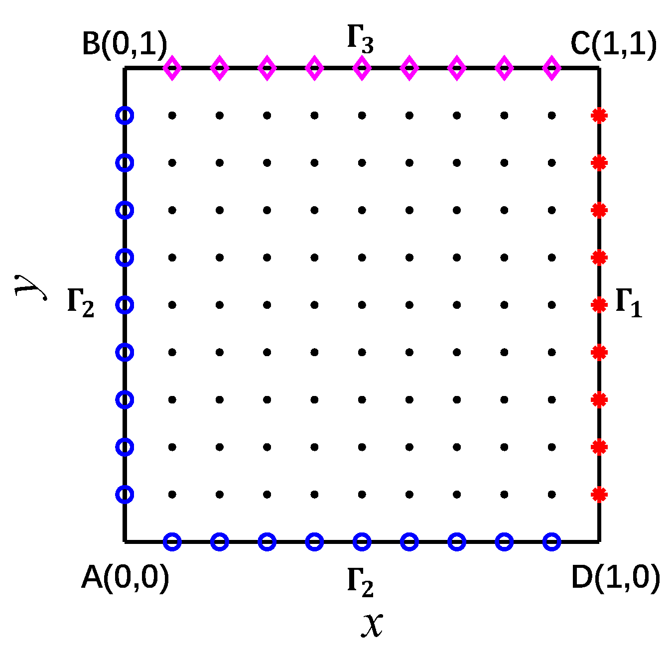
A nonlinear case in the previous work of Bialecki and Nowak is considered [49], where the two-dimensional heat conduction in the unit square Ω = [0, 1] × [0, 1] is shown in Figure 2. There is no radiation on the boundary Γ3. Assuming the thermal conductivity changes with temperature as follows:
K ( T ) = K 0 ( 1 + m ( T ) ) ,
where K(T) = 1 + aT constant is positive, a ≥ 0 is the prescribed positive constant, K0 = 1 is simply considered here:
f = 300   K ,   C h = 10   W / m K 2 ,   T f = 500   K ,   g = q = R = 0 .
Substituting Equation (32) to Equation (5), the following Kirchhoff transformation formula can be obtained:
Φ = φ ( T ) = T + T 2 2 ,
then the temperature can be obtained from Equation (34),
T = φ 1 ( Φ ) = 1 + 1 + 2 a Φ a ,
the governing equation and the boundary conditions can be described as,
2 Φ = 0 , in   Ω ,
Φ ( 1 , y ) = 300 ( 1 + 150 a ) , on Γ 1 ,
Φ x ( 0 , y ) = 0 , on Γ 2 ,
Φ y ( x , 0 ) = 0 , on Γ 2 ,
Φ y ( x , 1 ) + 10 [ 2 Φ ( x , 1 ) 1 + 1 + 2 a Φ ( x , 1 ) 500 ] = 0 , on Γ 3 ,
where a = 0, then K(T) = 1. The governing equation can be described as a linear governing equation as follows:
2 T = 0 , in Ω ,
with the boundary conditions,
T ( 1 ,   y ) = 300 , on Γ 1 ,
T x ( 0 , y ) = 0 , on Γ 2 ,
T y ( x , 0 ) = 0 , on Γ 2 ,
T y ( x , 1 ) + 10 ( T ( x , 1 ) 500 ) = 0 , on Γ 3 ,
9 × 9 = 81 nodes are uniformly distributed over the domain of Figure 2. The number of nodes in the local domain is fixed at 15.
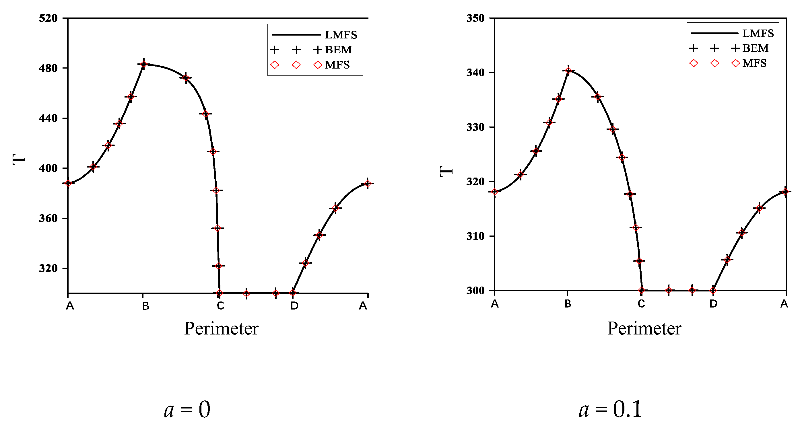
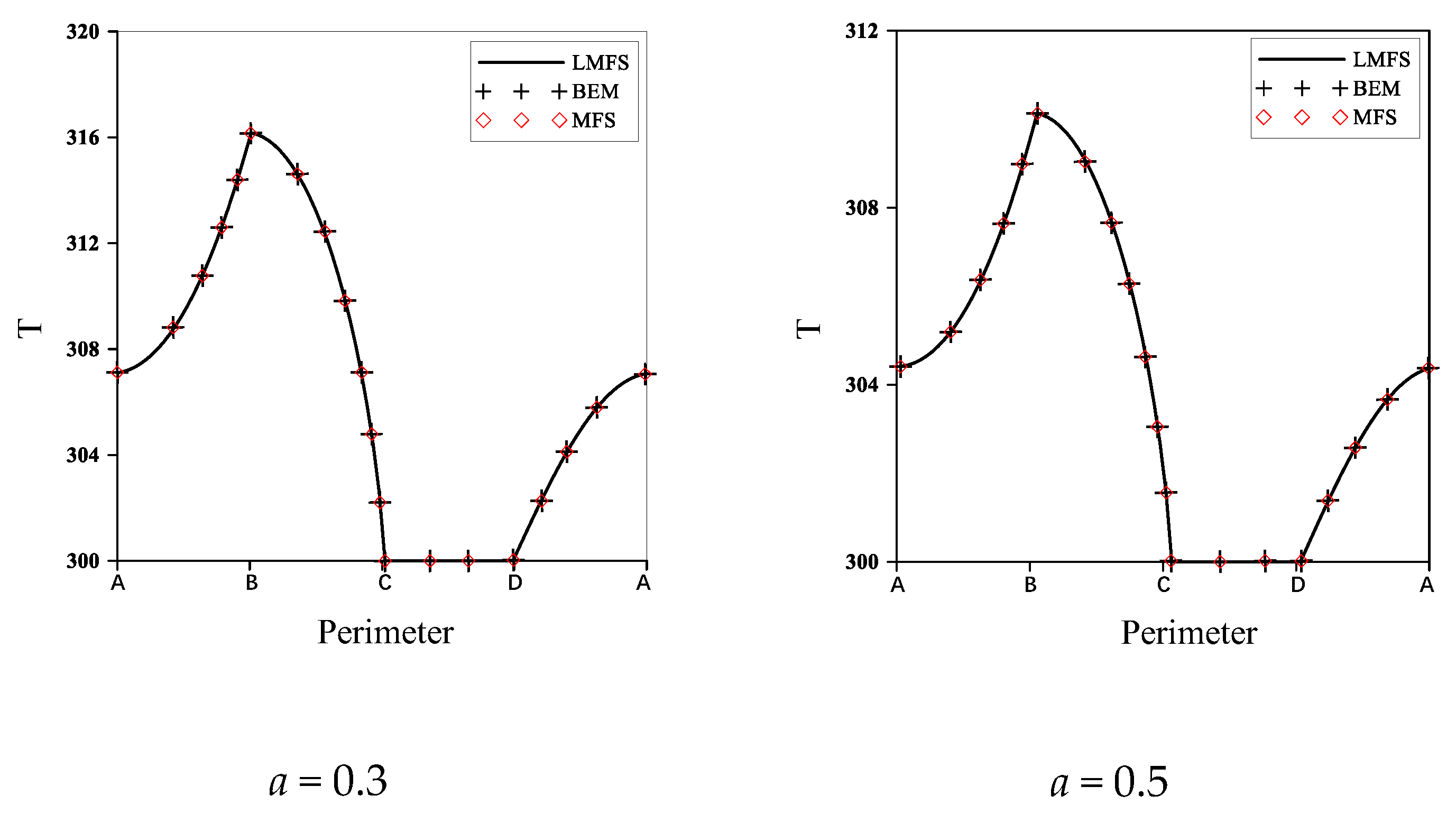
Since there are no exact solutions, the numerical results in this paper are compared with previous works [49,50]. In Figure 3, the temperature around the boundary is given, starting from the origin point A back to A in a clockwise direction in the case of a = 0, 0.1, 0.3, and 0.5. The total number of nodes is 117. As shown in points B, C, and D of Figure 3, there are monotonic changes of the temperature on the boundary, which is the same as the physical phenomenon [49]. The numerical results in Figure 3 fit well with the corresponding graphs obtained from MFS [49] and BEM [50]. In Figure 3, the problem is linear when a = 0, and the nonlinearity is increasing when the value of a is becoming large. Numerical results show that the LMFS can obtain good results in both linear and non-linear problem.

5.2. Example 2

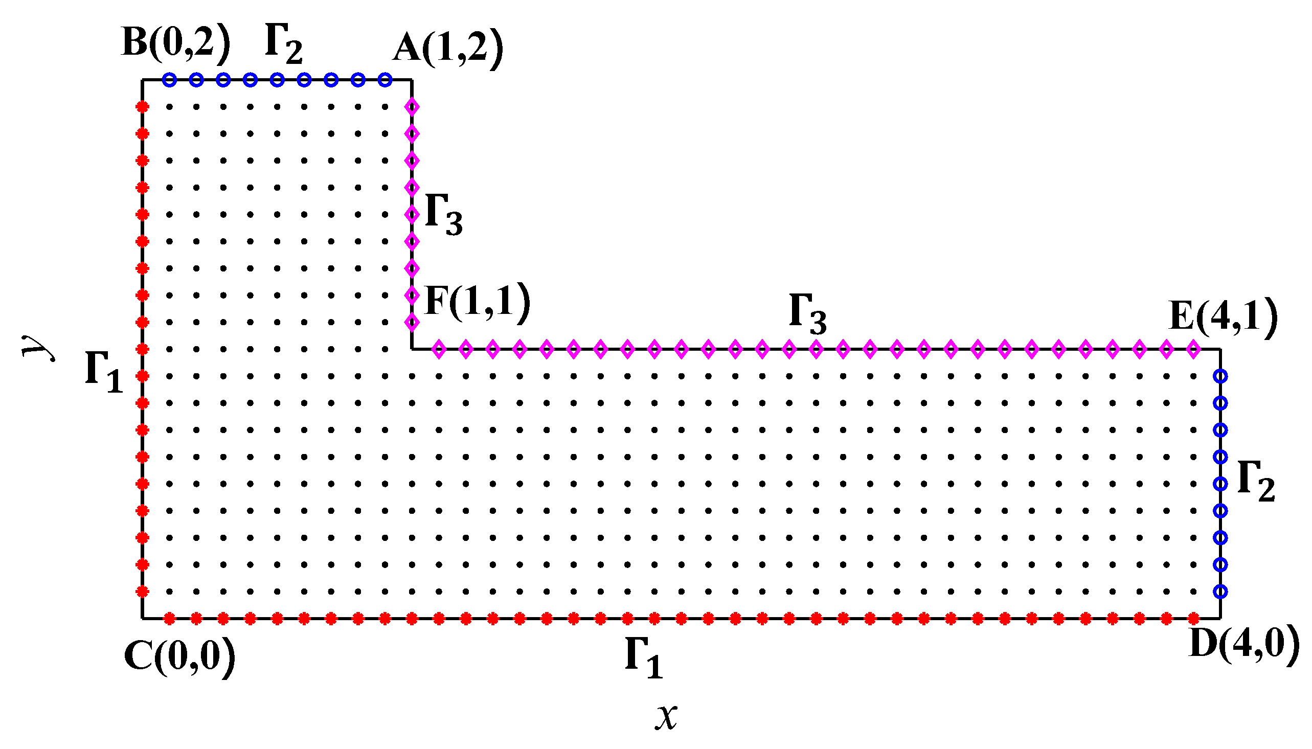
In this case, another case in the L domain is considered, as shown in Figure 4, where a totality of 555 nodes, including the 114 boundary nodes, are distributed:
K ( T ) = K 0 ( 1 + a T ) , K 0 = 1   W / m K , a = 0.25   K 1 ,
we consider the convective boundary conditions with a constant heat transfer coefficient Ch = 40 W/m2K, the thermal radiation interchange factor R = 0.7, f = 320 K, Ts = 1000 K, and g = q = 0. Employing the Kirchhoff transformation, the governing equation can be changed to:
2 Φ = 0 , in Ω ,
with the boundary conditions:
Φ ( x , y ) = 13 , 120 , on Γ 1 ,
Φ y ( x , 2 ) = Φ x ( 4 , y ) = 0 , on Γ 2 ,
Φ y ( x , 1 ) + N ( x , 1 ) = 0 , on Γ 3 ,
Φ y ( 1 , y ) + N ( 1 , y ) = 0 , on Γ 3 ,
where
N ( x , y ) = 160 [ 1 + 0.5 Φ ( x , y ) 126 ] + 3.967 × 10 8 [ 256 ( 1 + 1 + 0.5 Φ ( x , y ) ) 4 10 12 ] .
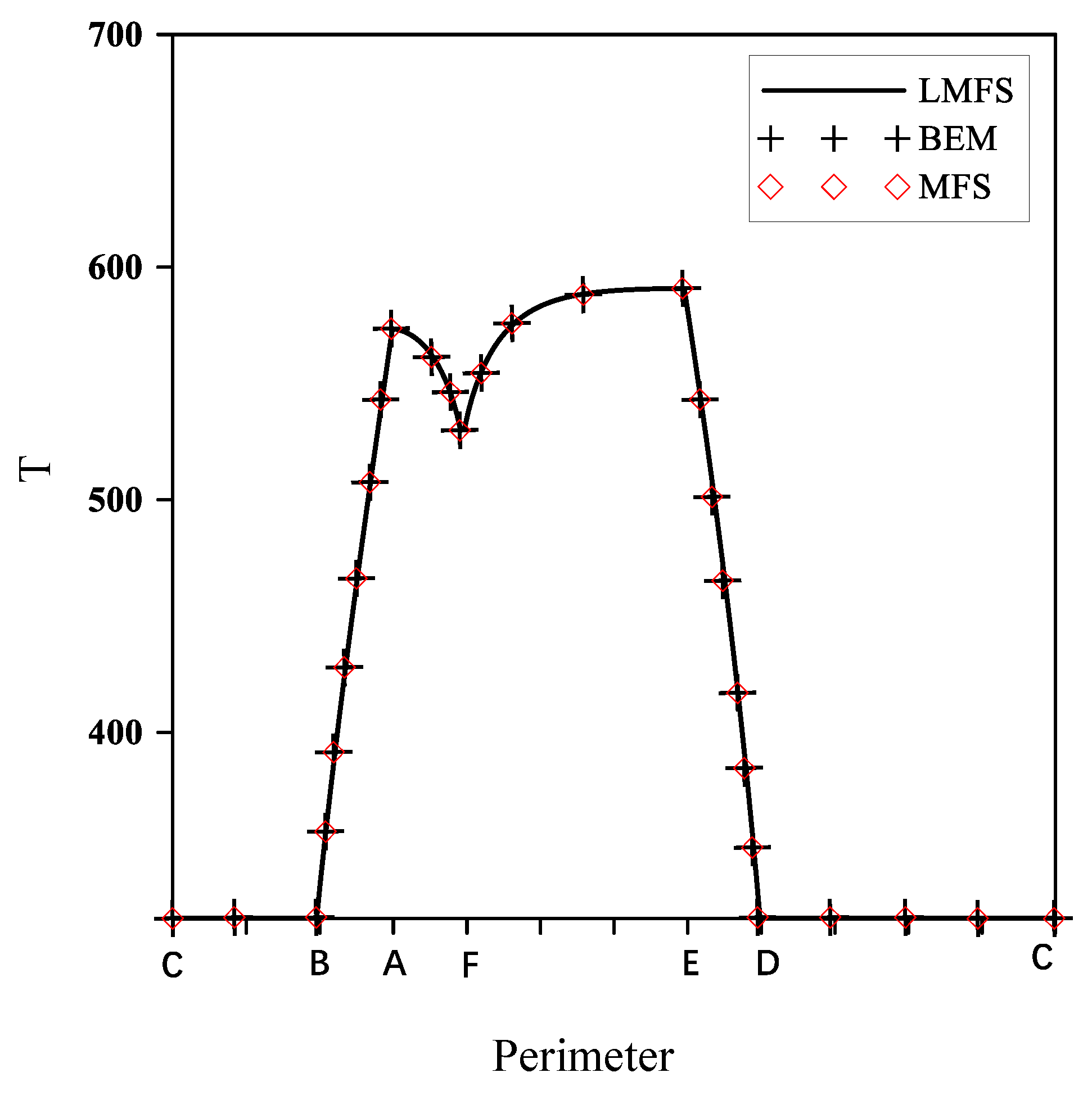
As there is no exact solution to this problem, the numerical results in this paper are compared with previous works [49,50]. In Figure 5, the temperature at the boundary is given, starting from the origin C, and back to C in a clockwise direction, as shown in Figure 4. In this case, the number of the local domain nodes is 15. The numerical results are given in Figure 5, where the temperatures on the boundary show sudden changes at points B, A, F, E, and D. The numerical results obtained from the LMFS have a similar phenomenon by comparing with the results of the MFS and BEM [49,50], which also validates the accuracy of the numerical results obtained from LMFS.
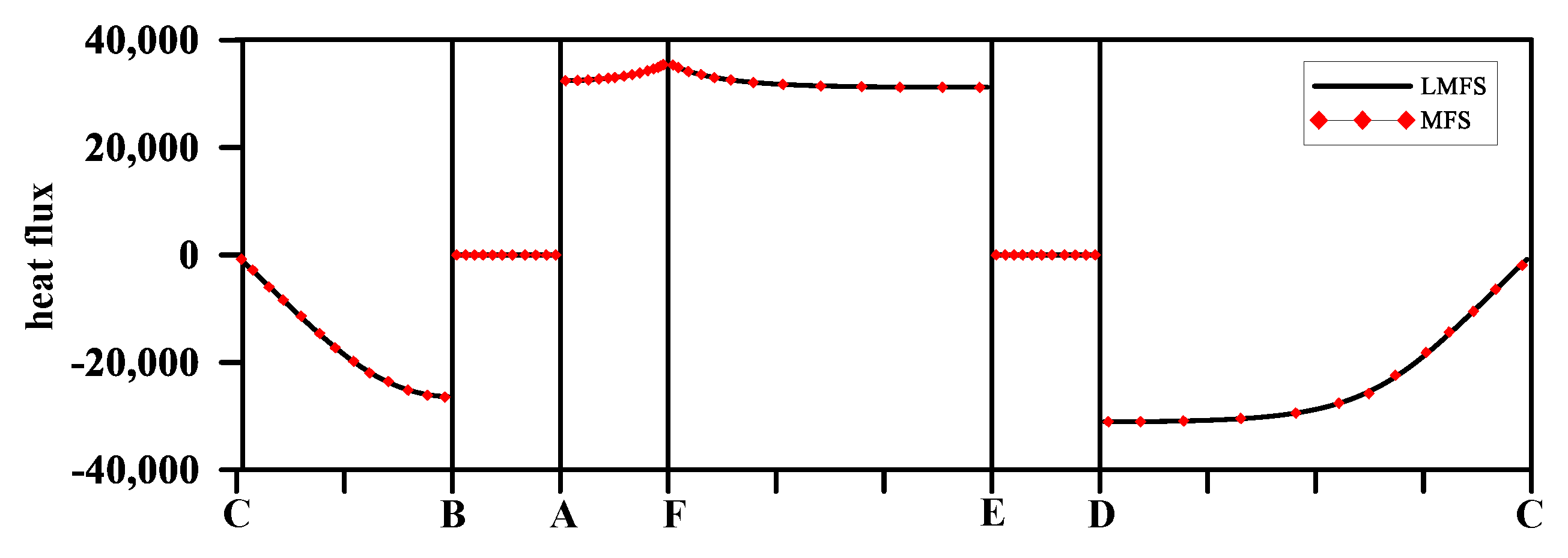
In Figure 6, we further give the heat flux when a = 0.25. As shown in Figure 6, there are huge variations of the heat flux at point B, A, E, and D. However, both the LMFS and the MFS [49] can obtain a similar numerical result at these points. The LMFS can evaluate the heat flux very well.

5.3. Example 3

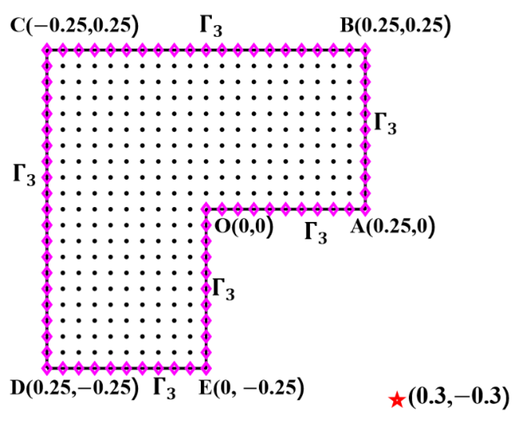
In order to analyze the influence of the nodes’ distribution, we consider a computational domain depicted in Figure 7, with an exact solution as:
T ( x , y ) = 1 + 1 2 a ln ( ( x 0.3 ) 2 + ( y + 0.3 ) 2 ) a
then
K ( T ) = K 0 ( 1 + a T ) , K 0 = 1   W / m K , a { 0.1 , 0.3 , 0.5 } K 1 ,
the radiation boundary conditions are given on all the boundaries as:
C h = 0 , R = 10 8 / 5.667 , T s = 0 ,
the boundary condition can be changed to:
K ( T ) T ( x , y ) n + ( T ( x , y ) ) 4 = q L , on Γ 3 ,
where qL is given as:
q L = ( 1 + a T ) n ( 1 + 1 2 a ln ( ( x 0.3 ) 2 + ( y + 0.3 ) 2 ) a ) + ( 1 + 1 2 a ln ( ( x 0.3 ) 2 + ( y + 0.3 ) 2 ) a ) 4 .
By employing the Kirchhoff transformation to the boundary condition, and the governing equation becomes:
2 Φ = 0 , in Ω ,
Φ ( x , y ) n + ( 1 + 1 + 2 a Φ ( x , y ) a ) 4 = q L 1 on Γ 3 ,
where
q L 1 = n ( ln ( ( x 0.3 ) 2 + ( y + 0.3 ) 2 ) ) + ( ln ( ( x 0.3 ) 2 + ( y + 0.3 ) 2 ) ) 4 ,
the exact solution of problem (57) and (58) can be presented as:
Φ ( x , y ) = ln ( ( x 0.3 ) 2 + ( y + 0.3 ) 2 ) , ( x , y ) ( Ω Γ 3 ) .
To generate the data qL1 in Equation (58), we use the derivatives:
x ( Φ ( x , y ) ) = x 0.3 ( x 0.3 ) 2 + ( y + 0.3 ) 2 ,  
y ( Φ ( x , y ) ) = y + 0.3 ( x 0.3 ) 2 + ( y + 0.3 ) 2 .
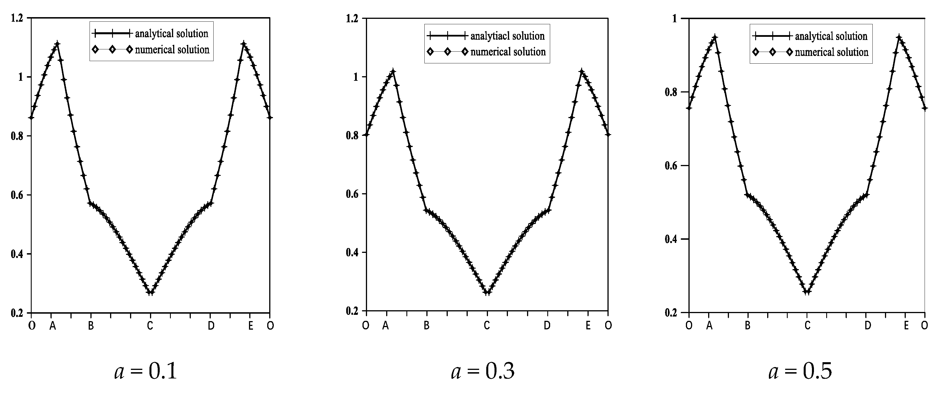
We present the boundary temperature along the boundary of case 3 in Figure 8; the number of local domain nodes is 10, and the total number of computational domain nodes is 347. It can be seen that the numerical solutions are in good agreement with the analytical solutions in Equation (53). It also can be seen that the temperature distribution along the boundary is symmetrical from point C.
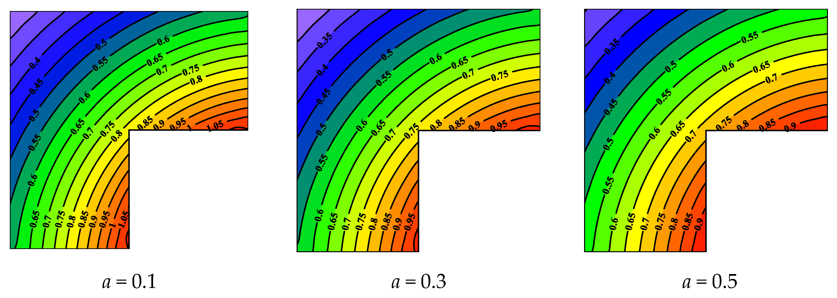
In Figure 9, we give the temperature contour map, when a = 0.1, 0.3, 0.5. We can see that the temperature contour distribution in the entire domain is symmetrical along the axis of the line between the points O and C, which is consistent with the physical heat transfer law. As the value of a increases, the temperature in the calculation domain gradually decreases, which indicates that the larger value of a will lead to a lower temperature, which is consistent with Equation (52).
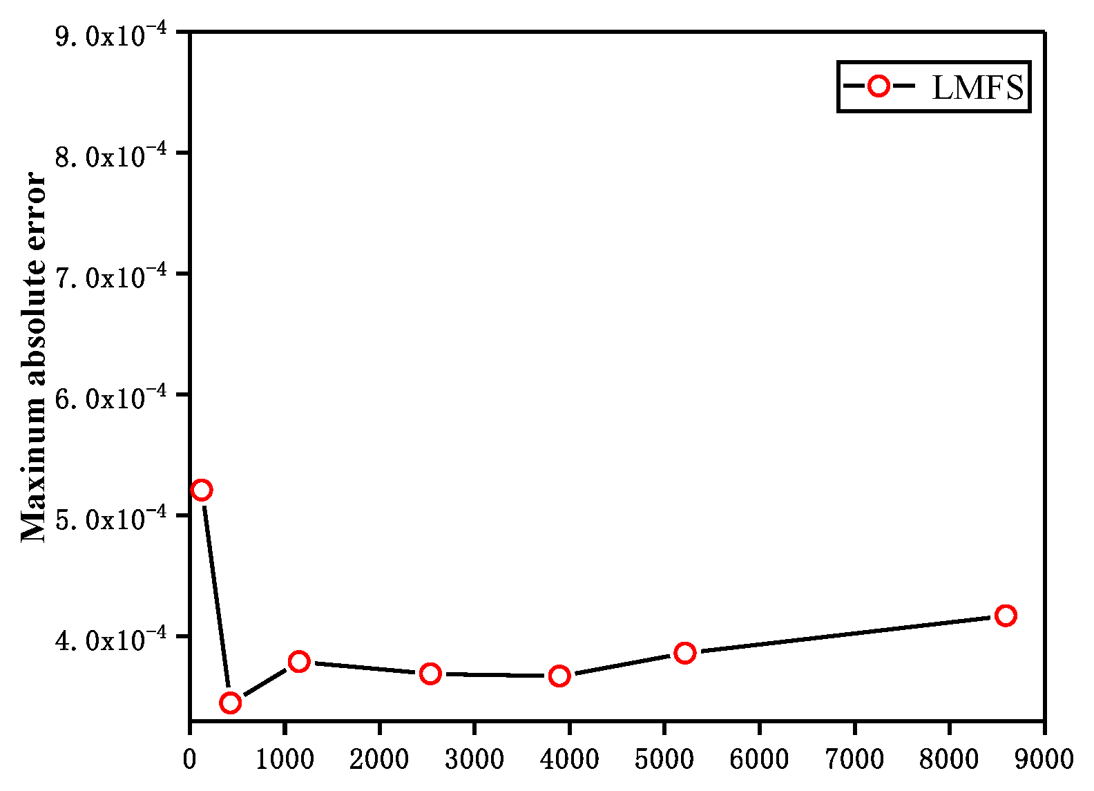
Finally, when the number of local domain nodes is fixed at 15, the convergence rate is given in Figure 10, where Na is the total number of nodes. From the numerical results in Figure 10, we can see that the maximum absolute error defined in Equation (31) obtained from the LMFS convergences after Na = 300. As the number of nodes increases after Na = 300, the maximum absolute error increases; however, the maximum absolute error still retains a high accuracy.

5.4. Example 4

Finally, we analyze the influence of the local nodes by considering a simple, three-dimensional case with exact solution:
T ( x , y , z ) = 4 ( 1 + 1 + x + y + z ) , ( x , y , z ) ( 0 , 1 ) 3 ,
the nonlinear materials with thermal conductivity:
K ( T ) = K 0 ( 1 + a T ) , K 0 = 1 W / m K , a = 0 . 25 K 1 .
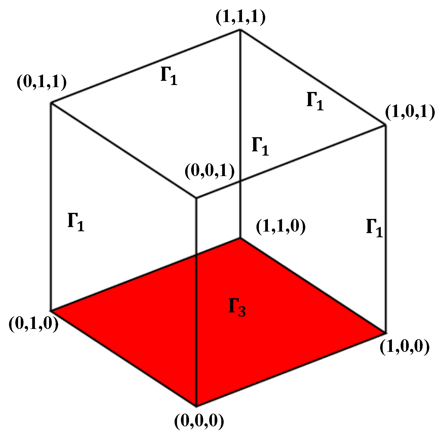
We distribute nodes uniformly in the computational domain, as shown in the Figure 11; we take Ch = Ts = 0 and R = 4,411,500. Based on Equation (5), boundary conditions in Equations (2)–(4) become:
T ( 0 , y , z ) = 4 ( 1 + 1 + y + z ) , T ( 1 , y , z ) = 4 ( 1 + 2 + y + z ) ,
T ( x , 0 , z ) = 4 ( 1 + 1 + x + z ) , T ( x , 1 , z ) = 4 ( 1 + 2 + x + z ) ,
T ( x , y , 1 ) = 4 ( 1 + 2 + x + z ) ,
( 1 + T ( x , y , 0 ) 4 ) T z ( x , y , 0 ) + T 4 ( x , y , 0 ) = 2 + 256 ( 1 + 1 + x + y ) 4 ,
considering the Kirchhoff transformation, we can obtain:
Φ = φ ( T ) = T + T 2 8 , T = φ 1 ( Φ ) = 4 ( 1 + 1 + Φ / 2 ) ,
and the governing equation is changed to:
2 Φ ( x , y , z ) = 0 , ( x , y , z ) ( 0 , 1 ) 3 ,
with boundary conditions:
Φ ( 0 , y , z ) = 2 ( y + z ) , Φ ( 1 , y , z ) = 2 ( 1 + y + z ) ,
Φ ( x , 1 , z ) = 2 ( 1 + x + z ) , Φ ( x , y , 1 ) = 2 ( 1 + x + y ) ,
Φ z ( x , y , 0 ) + 256 ( 1 + 1 + Φ ( x , y , 0 ) / 2 ) 4 = 2 + 256 ( 1 + 1 + x + y ) 4 .
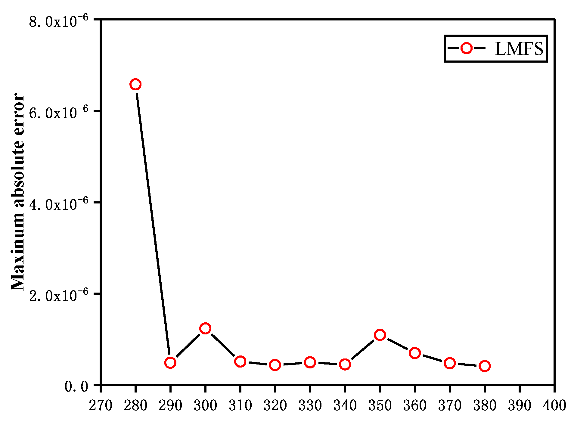
In Figure 12, we test the influence of the number of local nodes when the total number of nodes is fixed at 3547. It can be seen that, when the total number of nodes is fixed, the maximum absolute decreases with the increase of the number of local nodes, the error of the LMFS solution is small when the number of local nodes is over 290.

6. Conclusions

In this work, the local method of fundamental solution (LMFS) is used to solve two-dimensional and three-dimensional steady-state nonlinear heat conduction problems. The numerical results show that the LMFS can be easily used to solve steady-state nonlinear heat conduction problems with Robin and radiation boundary conditions. The LMFS combined with the Kirchhoff transformation can deal with the nonlinearity very well and obtain high numerical results. In our future work, we will apply the LMFS to more complicated nonlinear problems based on the techniques proposed in this work.

Author Contributions

Data curation, H.Z.; Formal analysis, F.W.; Methodology, Y.-C.L. All authors have read and agreed to the published version of the manuscript.

Funding

This research received no external funding.

Institutional Review Board Statement

Not applicable.

Informed Consent Statement

Not applicable.

Data Availability Statement

Not applicable.

Acknowledgments

This work is supported by the National Natural Science Foundation of China (No: 12172159), National Natural Science Foundation of Jiangxi Provence (No: 20192ACB21022; 20212BAB211022), Jiangxi Province Funds for Distinguished Young Scientists (No: 20192ACB21022). The authors are very thankful for Jiangxi double thousand talents support (No: jxsq2018106027).

Conflicts of Interest

The authors declare no conflict of interest.

References

  1. Bagnall, K.R.; Muzychka, Y.S.; Wang, E.N. Application of the Kirchhoff transform to thermal spreading problems with convection boundary conditions. IEEE Trans. Compon. Packag. Manuf. Technol. 2014, 4, 408–420. [Google Scholar] [CrossRef]
  2. Mosayebidorcheh, S.; Ganji, D.D.; Farzinpoor, M. Approximate solution of the nonlinear heat transfer equation of a fin with the power-law temperature-dependent thermal conductivity and heat transfer coefficient. Propuls. Power Res. 2014, 3, 41–47. [Google Scholar] [CrossRef] [Green Version]
  3. Moradi, A.; Ahmadikia, H. Analytical solution for different profiles of fin with temperature-dependent thermal conductivity. Math. Probl. Eng. 2010, 15, 568263. [Google Scholar] [CrossRef]
  4. Ghasemi, S.E.; Hatami, M.; Ganji, D.D. Thermal analysis of convective fin with temperature-dependent thermal conductivity and heat generation. Case Stud. Therm. Eng. 2014, 4, 1–8. [Google Scholar] [CrossRef] [Green Version]
  5. Chang, J.Y.; Tsai, C.C.; Young, D.L. Homotopy method of fundamental solutions for solving nonlinear heat conduction problems. Eng. Anal. Bound. Elem. 2019, 108, 179–191. [Google Scholar] [CrossRef]
  6. Mitchell, A.R.; Griffiths, D.F. The Finite Difference Method in Partial Differential Equations; John Wiley: New York, NY, USA, 1980. [Google Scholar]
  7. Warming, R.F.; Hyett, B.J. The Modified Equation Approach to the Stability and Accuracy of Finite Difference Method. J. Comput. Phys. 1974, 14, 159–179. [Google Scholar] [CrossRef]
  8. Strang, G.; Fix, G.J.; Griffin, D.S. An Analysis of the Finite Element Method; Prentice-Hall: Englewood Cliffs, NJ, USA, 1973. [Google Scholar]
  9. Qiang, C.; Wang, G.; Jerzy, P.M. Homogenization and localization of nanoporous composites-A critical review and new developments. Compos. Part B Eng. 2018, 155, 329–368. [Google Scholar]
  10. Uwe, M.; Georgios, P. Mechanism based diffusion-reaction modelling for predicting the influence of SARA composition and ageing stage on spurt completion time and diffusivity in bitumen. Constr. Build. Mater. 2021, 267, 120592. [Google Scholar]
  11. Bialecki, R.; Kuhn, G. Boundary element solution of heat conduction problems in multizone bodies of non-linear material. Int. J. Numer. Methods Eng. 1993, 36, 799–809. [Google Scholar] [CrossRef]
  12. Cavalcante, M.; Marques, S.; Pindera, M.J. Parametric Formulation of the Finite-Volume Theory for Functionally Graded Materials—Part I: Analysis. J. Appl. Mech. 2007, 74, 935. [Google Scholar] [CrossRef]
  13. Versteeg, H.K.; Malalasekera, W. An Introduction to Computational Fluid Dynamics; Pearson education: Upper Saddle River, NJ, USA, 1996. [Google Scholar]
  14. Oliveira, P.J.; Pinho, F.T.; Pinto, G.A. Numerical simulation of non-linear elastic flows with a general collocated finite-volume method. J. Non-Newton. Fluid Mech. 1998, 79, 1–43. [Google Scholar] [CrossRef] [Green Version]
  15. Zheng, H.; Sladek, J.; Sladek, V.; Wen, P.H. Fracture analysis of functionally graded material by hybrid meshless displacement discontinuity method. Eng. Fract. Mech. 2021, 247, 107591. [Google Scholar] [CrossRef]
  16. Zheng, H.; Zhou, C.B.; Yan, D.J.; Wang, Y.S.; Zhang, C.Z. A meshless collocation method for band structure simulation of nanoscale phononic crystals based on nonlocal elasticity theory. J. Comput. Phys. 2020, 408, 109268. [Google Scholar] [CrossRef]
  17. Zheng, H.; Sladek, J.; Sladek, V.; Wen, P.H. Hybrid meshless/displacement discontinuity method for FGM Reissner’s plate with cracks. Appl. Math. Model. 2021, 90, 1226–1244. [Google Scholar] [CrossRef]
  18. Zheng, H.; Wang, F.; Chen, C.S.; Lei, M.; Wang, Y. Improved 3D surface reconstruction via the method of fundamental solutions. Numer. Math. Theory Methods Appl. 2020, 13, 973–985. [Google Scholar] [CrossRef]
  19. Sun, P.N.; Colagrossi, A.; Touzé, D.L.; Zhang, A.M. Extension of SPH model for simulating Vortex-Induced-Vibration problems. J. Fluids Struct. 2019, 90, 19–42. [Google Scholar] [CrossRef]
  20. Li, Q.H.; Chen, S.S.; Kou, G.X. Transient heat conduction analysis using the MLPG method and modified precise time step integration method. J. Comput. Phys. 2011, 230, 2736–2750. [Google Scholar] [CrossRef]
  21. Tsai, C.C. Homotopy method of fundamental solutions for solving certain nonlinear partial differential equations. Eng. Anal. Bound. Elem. 2012, 36, 1226–1234. [Google Scholar] [CrossRef]
  22. Chati, M. The boundary node method for three-dimensional linear elasticity. Int. J. Numer. Methods Eng. 2015, 46, 1163–1184. [Google Scholar] [CrossRef]
  23. Tan, G.; Wang, H.; Song, C. 2-D simulation of electrostatic properties of piezoelectric composites using the boundary node method. J. Tsinghua Univ. 2007, 5, 734–737. [Google Scholar]
  24. Fan, C.M.; Chan, H.F.; Kuo, C.L. Numerical solutions of boundary detection problems using modified collocation Trefftz method and exponentially convergent scalar homotopy algorithm. Eng. Anal. Bound. Elem. 2012, 36, 2–8. [Google Scholar] [CrossRef]
  25. Fan, C.M.; Young, D.L.; Chiu, C.L. Method of Fundamental Solutions with External Source for the Eigenfrequencies of Waveguides. J. Mar. Sci. Technol. 2009, 17, 164–172. [Google Scholar] [CrossRef]
  26. Gu, Y.; Wen, C.; Zhang, C.Z. Singular boundary method for solving plane strain elastostatic problems. Int. J. Solids Struct. 2011, 48, 2549–2556. [Google Scholar] [CrossRef] [Green Version]
  27. Fu, Z.J.; Wen, C.; Lin, J. Singular Boundary Method for Various Exterior Wave Applications. Int. J. Comput. Methods 2015, 12, 1550011. [Google Scholar] [CrossRef]
  28. Chen, C.S.; Golberg, M.A.; Hon, Y.C. The method of fundamental solutions and quasi-Monte-Carlo method for diffusion equations. Int. J. Numer. Methods Eng. 2015, 43, 1421–1435. [Google Scholar] [CrossRef]
  29. Young, D.L.; Wu, J.T.; Chiu, C.L. Method of Fundamental Solutions for Stokes Problems by the Pressure-Stream Function Formulation. J. Mech. 2008, 24, 137–144. [Google Scholar] [CrossRef]
  30. Zheng, H.; Yang, Z.J.; Zhang, C.Z.; Tyrer, M. A local radial basis function collocation method for band structure computation of phononic crystals with scatterers of arbitrary geometry. Appl. Math. Model. 2018, 60, 447–459. [Google Scholar] [CrossRef]
  31. Zheng, H.; Zhang, C.Z.; Wang, Y.S.; Chen, W.; Sladek, J.; Sladek, V. A local RBF collocation method for band structure computations of 2D solid/fluid and fluid/solid phononic crystals. Int. J. Numer. Methods Eng. 2017, 110, 467–500. [Google Scholar] [CrossRef]
  32. Kupradze, V.D.; Aleksidze, M.A. The method of functional equations for the approximate solution of certain boundary value problems. Ussr Comput. Math. Math. Phys. 1964, 4, 82–126. [Google Scholar] [CrossRef]
  33. Fan, C.M.; Chen, C.S.; Monroe, J. The Method of Fundamental Solutions for Solving Convection-Diffusion Equations with Variable Coefficients. Adv. Appl. Math. Mech. 2009, 1, 215–230. [Google Scholar]
  34. Mainardi, F. The fundamental solutions for the fractional diffusion-wave equation. Appl. Math. Lett. 1996, 9, 23–28. [Google Scholar] [CrossRef] [Green Version]
  35. Yan, L.; Fu, C.; Yang, F. The method of fundamental solutions for the inverse heat source problem. Eng. Anal. Bound. Elem. 2008, 32, 216–222. [Google Scholar] [CrossRef]
  36. Fan, C.M.; Huang, Y.K.; Chen, C.S. Localized method of fundamental solutions for solving two-dimensional Laplace and biharmonic equations. Eng. Anal. Bound. Elem. 2019, 101, 188–197. [Google Scholar] [CrossRef]
  37. Qu, W.; Fan, C.M.; Gu, Y. Analysis of three-dimensional interior acoustic fields by using the localized method of fundamental solutions. Appl. Math. Model. 2019, 76, 122–132. [Google Scholar] [CrossRef]
  38. Li, W. Localized method of fundamental solutions for 2D harmonic elastic wave problems. Appl. Math. Lett. 2021, 112, 106759. [Google Scholar] [CrossRef]
  39. Reutskiy, S. The method of fundamental solutions for Helmholtz eigenvalue problems in simply and multiply connected domains. Eng. Anal. Bound. Elem. 2006, 30, 150–159. [Google Scholar] [CrossRef]
  40. Wang, X.; Gu, Y.; Golub, M.V. Analysis of bimaterial interface cracks using the localized method of fundamental solutions. Results Math. 2022, 13, 100231. [Google Scholar] [CrossRef]
  41. Alves, C.; Antunes, P. The Method of Fundamental Solutions applied to the calculation of eigensolutions for simply connected plates. Int. J. Numer. Methods Eng. 2006, 77, 177–194. [Google Scholar] [CrossRef]
  42. Tsai, C.C. The method of fundamental solutions with dual reciprocity for three-dimensional thermoelasticity under arbitrary body forces. Eng. Comput. 2009, 26, 229–244. [Google Scholar] [CrossRef]
  43. Carslaw, H.; Jaeger, J. Conduction of Heat in Solids; Oxford Science Publications: Oxford, UK, 1959. [Google Scholar]
  44. Barnett, T.L. Application of a Nonlinear Least-Squares Method to Atmospheric Temperature Sounding. J. Atmos. Sci. 1969, 26, 457–461. [Google Scholar] [CrossRef] [Green Version]
  45. Blaha, G.; Bessette, R.P. Nonlinear least-squares method via an isomorphic geometrical setup. Bull. Geod. 1989, 63, 115–137. [Google Scholar] [CrossRef]
  46. Fernandez, M.A.; Moubachir, M. A Newton method using exact jacobians for solving fluid-structure coupling. Comput. Struct. 2005, 83, 127–142. [Google Scholar] [CrossRef] [Green Version]
  47. Liu, C.S. A fictitious time integration method for two-dimensional quasi-linear elliptic boundary value problems. Comput. Modeling Eng. Sci. 2008, 33, 179–198. [Google Scholar]
  48. Liu, C.S. A fictitious time integration method for a quasilinear elliptic boundary value problem, defined in an arbitrary plane domain. Comput. Mater. Contin. 2009, 11, 15–32. [Google Scholar]
  49. Karageorghis, A.; Lesnic, D. The Method of Fundamental Solutions for Steady-State Heat Conduction in Nonlinear Materials. Commun. Comput. Phys. 2008, 4, 911–928. [Google Scholar] [CrossRef]
  50. Bialecki, R.; Nowak, A.J. Boundary value problems in heat conduction with nonlinear material and nonlinear boundary conditions. Appl. Math. Model. 1981, 5, 417–421. [Google Scholar] [CrossRef]
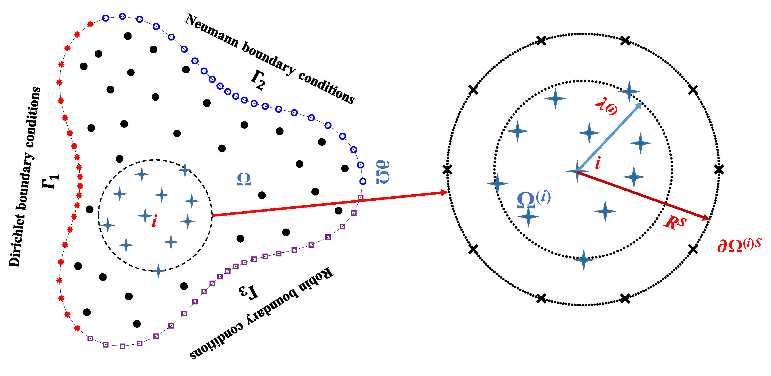
Figure 1. The local domain of the ith node from a global domain.
Mathematics 10 00773 g001
Figure 2. Schematic of the computational domain of case 1.
Mathematics 10 00773 g002
Figure 3. The boundary temperature when a = 0, 0.1, 0.3, 0.5.
Mathematics 10 00773 g003aMathematics 10 00773 g003b
Figure 4. Schematic of the computational domain of case 2.
Mathematics 10 00773 g004
Figure 5. The boundary temperature when a = 0.25.
Mathematics 10 00773 g005
Figure 6. The heat flux on the boundary when a = 0.25.
Mathematics 10 00773 g006
Figure 7. Schematic of the computational domain of case 3.
Mathematics 10 00773 g007
Figure 8. Plot of analytical and the LMFS numerical boundary temperatures along the perimeter, case a = 0.1, 0.3, 0.5.
Mathematics 10 00773 g008
Figure 9. Contour map of temperature in the calculation domain, when a = 0.1, 0.3, 0.5.
Mathematics 10 00773 g009
Figure 10. The convergence rate of the total nodes.
Mathematics 10 00773 g010
Figure 11. Schematic of the computational domain.
Mathematics 10 00773 g011
Figure 12. The convergence rate of local nodes.
Mathematics 10 00773 g012
Publisher’s Note: MDPI stays neutral with regard to jurisdictional claims in published maps and institutional affiliations.