Revisiting the Copula-Based Trading Method Using the Laplace Marginal Distribution Function

Abstract

Pairs trading under the copula approach is revisited in this paper. It is well known that financial returns arising from indices in markets may not follow the features of normal distribution and may exhibit asymmetry or fatter tails, in particular. Due to this, the Laplace distribution is employed in this work to fit the marginal distribution function, which will then be employed in a copula function. In fact, a multivariate copula function is constructed on two indices (based on the Laplace marginal distribution), enabling us to obtain the associated probabilities required for the process of pairs trade and creating an efficient tool for trading.

1. Introduction

Taking the Basel Committee documents into consideration, we divide the risk for business into five main parts [1]: 1. The risk of country, which contains the lack of certainties of political systems and the internal dynamics of societies. 2. The risk of settlement, which contains the external uncertainties of running finance processes along with the operating sequences. 3. The market risk that includes the fuzziness of factors inside markets in association with the valuation and price mechanisms. 4. The credit risk that contains the lack of certainty for external economical effects on sources required from the economic environment. 5. The operational risk, which relates to the structures and parameters of internal organizational processes in connection to individual failures and misbehavior. Hence, managing risk or reinvestigating well-known algorithmic methods is of interest in mathematical finance [2,3].

We name a multidimensional cumulative distribution function (CDF) as a copula, when each variable has a uniform marginal probability distribution on [0,1]. These functions are employed to illustrate the dependency of several given stochastic variables. In fact, they have broadly been employed in multivariate statistics and quantitative finance ranging from trading in portfolios with several stocks to risk management [4,5,6].

Perhaps the most fundamental finding for copulas is the theorem given by Sklar in [7], which mentions that any multidimensional joint distribution could be obtained via one-dimensional marginal distribution functions along with a copula function that shows the structure of dependency among several variables. These distributions were first introduced in the 1940s, and their related machinery and terminology were improved in the 1950s and 1960s [8].

Mostly, Archimedean copulas, unlike the Gaussian copula, possess an explicit formula. They have been widely employed because of their mathematical tractability and also their ability to cover broad range of dependency. For a continuous and decreasing function

$$\psi :[0,\infty )\to [0,1],$$

(1)

with the conditions

$$\psi \left(0\right)=1,\psi (+\infty )=0,$$

(2)

and $\psi ={\varphi }^{-1}$ being the pseudo-inverse [7], we have:

$$C_{\psi }(u_1,u_2,\dots ,u_n)=\psi (\varphi \left(u_1\right)+\varphi \left(u_2\right)+\cdots +\varphi \left(u_n\right)),$$

(3)

$$\mathrm{for}\mathrm{any}{u}_i\in [0,1],i=1,2,\dots ,n,$$

which is an Archimedean copula having $\psi$ as the generator when

$${(-1)}^k{\psi }^{\left[k\right]}\left(x\right)\ge 0,$$

for all $k=0,1,\dots ,n-2$. Here, $\varphi (·)$ is the cumulative of the (standard normal) distribution, and

$${(-1)}^{n-2}{\psi }^{[n-2]}\left(x\right),$$

is convex and decreasing. The function (3) consists of several famous copulas including the Ali-Mikhail-Haq (AMH) copula, the Clayton copula, and the independence (product) copula [8].

In general, if there are two known marginal continuous distributions we cannot derive their joint distribution, but we can recover a joint distribution using a copula function. One of the merits of employing copulas is their isolation of the structure of dependence from the structure of the marginal distributions, etc. The marginal distribution may capture different types of symmetries, asymmetries, fat tails, and structural breaks with a strong influence on the estimation results for modeling of the dependence structure. A copula enables us to separate the joint distribution into the marginal distributions of each variable. This separation enables us to model the dependency among the variables directly.

We recall that it is necessary to use nonparametric measures, such as Kendall’s $\tau$ or Spearman’s $\rho$ (Spearman’s correlation coefficient) [8], in several practical cases, since the basic Pearson correlation coefficient measures the linear dependence only.

Consider the parameter $\rho \in [-1,1]$; then, the unique bivariate normal (or Gauss, or Gaussian) copula is given via the use of the Sklar’s theorem as follows:

$$C(u_1,u_2;\rho )={\varphi }_2({\varphi }^{-1}\left(u_1\right),{\varphi }^{-1}\left(u_2\right);\rho ),$$

(4)

where ${\varphi }_2(·)$ is the CDF of the bivariate standard normal distribution. Note that for $\rho =\{-1,1\}$, the correlation matrix of the two-dimensional standard normal distribution becomes singular. The Gaussian copula (4) is flexible in the sense that it useful for both negative and positive dependency. The correlation parameter $\rho$ is given as:

$$\rho =sin\left(\frac{\pi }{2}\mathrm{Kendall}’\mathrm{s}\tau \right),$$

(5)

wherein

$${\displaystyle \mathrm{Kendall}’\mathrm{s}\tau =4\int \int C(u_1,u_2)dC(u_1,u_2)-1.}$$

(6)

Sometimes, two-dimensional copulas are named doubly-stochastic measures.

In this work, we investigate how to construct a copula with Laplace marginal distribution function. The constructed copula is then be employed on pair trading (also known as pairs trading) as an efficient trading method in quantitative finance.

The Laplace distribution has been shown to provide better fits on economic and financial data when compared to the famous normal distribution [9]. So, this is employed herein as a good tool for managing risk. In fact, the motivation behind choosing the Laplace distribution for risk management is the point that this distribution leads to fatter tails (in contrast to normal distribution tails), which matches much more preferably with the observations of the market [10].

The remainder of this paper is organized as follows. In Section 2, the Laplace distribution is defined briefly. Next, in Section 3, the pairs trading strategy is given briefly. A trading algorithm is furnished in Section 4 as an efficient tool for risk managers and traders. Further simulation results and comparisons are described in Section 5. They confirm the applicability of the Laplace marginal distribution function in contrast to the normal distribution for risk management. Section 6 ends the paper with a conclusion and future focuses.

2. Laplace Distribution

The Laplace distribution is the distribution of differences between two independent variates with identical exponential distributions. In fact, the difference between two independent identically distributed exponential random variables is controlled by a Laplace distribution, as is a Brownian motion computed at an exponentially distributed random time. This distribution is employable in situations wherein the lower values originate under different external conditions than the higher ones such that they follow a different pattern, see [11,12] for further discussions.

It is useful in predicting when a fatter tail (in contrast to normal distribution tails) on the underlying prices exists in the market and to express very different events [13,14]. The statistical continuous Laplace distribution with $\mu$ as the mean and $\sigma$ as the scale parameter is defined over the set of real numbers. Here, if

$$X\sim \mathrm{Laplace}(\mu ,\sigma ),$$

then its probability density function (PDF) is provided by:

$$f\left(x\right)=\left\{\begin{array}{cc}{\displaystyle \frac{e^{\frac{\mu -x}{\sigma }}}{2\sigma }},\hfill & x\ge \mu ,\hfill \\ {\displaystyle \frac{e^{\frac{x-\mu }{\sigma }}}{2\sigma }},\hfill & x<\mu .\hfill \end{array}\right.$$

(7)

Note that this distribution has a specific position along the normal distribution, being stable under geometric rather than ordinary summation; therefore, it is appropriate for stochastic modeling [13].

3. A Review of Pairs Trade

It is known that pairs trade is a famous strategy for trading broadly employed by investment banks and hedge funds [15]. This statistical arbitrage and convergence trading strategy is able to obtain profits irrespective of the direction of the market. It is derived via two steps. In the first step, an asset pair whose prices historically have moved with each other is detected. In the second step, by considering that in the future this equilibrium relationship should persist, the spread between the values of the stocks are controlled over a period of time. Furthermore, the investor shorts the overvalued asset and buys the undervalued one, when this deviates from its historical mean. After the price convergence, the positions are closed.

In the literature for the first part, two procedures are basically recommended. One is to perform a complete search for all available candidates among the chosen securities [16]. The second is to cluster them based on unsupervised machine learning techniques such as k-means++ and then constrain the groups into pairs. However, we consider here that we have already chosen these two appropriate pairs. In fact, pairs trading can be implemented after constructing an efficient portfolio via the clustering analysis procedure in unsupervised machine learning when the stocks of a portfolio have been clustered based on their associated risks, see the recent work [17] for further information.

In pairs trading based on copula theory, the pairs choice stage determines the suitable candidate pairs, choosing the promising ones. Starting with the quest for suitable pairs, the trader must choose the appropriate pairs.

4. An Algorithm Based on the Laplace Distribution

The two stocks considered for imposing the copula distribution function with the Laplace marginal distribution function are shown in

Table 1. Features of the equity pair considered for pairs trade. The dates on which the data were gathered, the copula function was constructed, and the prediction was calculated are provided.

Title	Symbol of Ticker	Market	Sector	Floating Shares	In-Sample Formation Period	Out of Sample Period
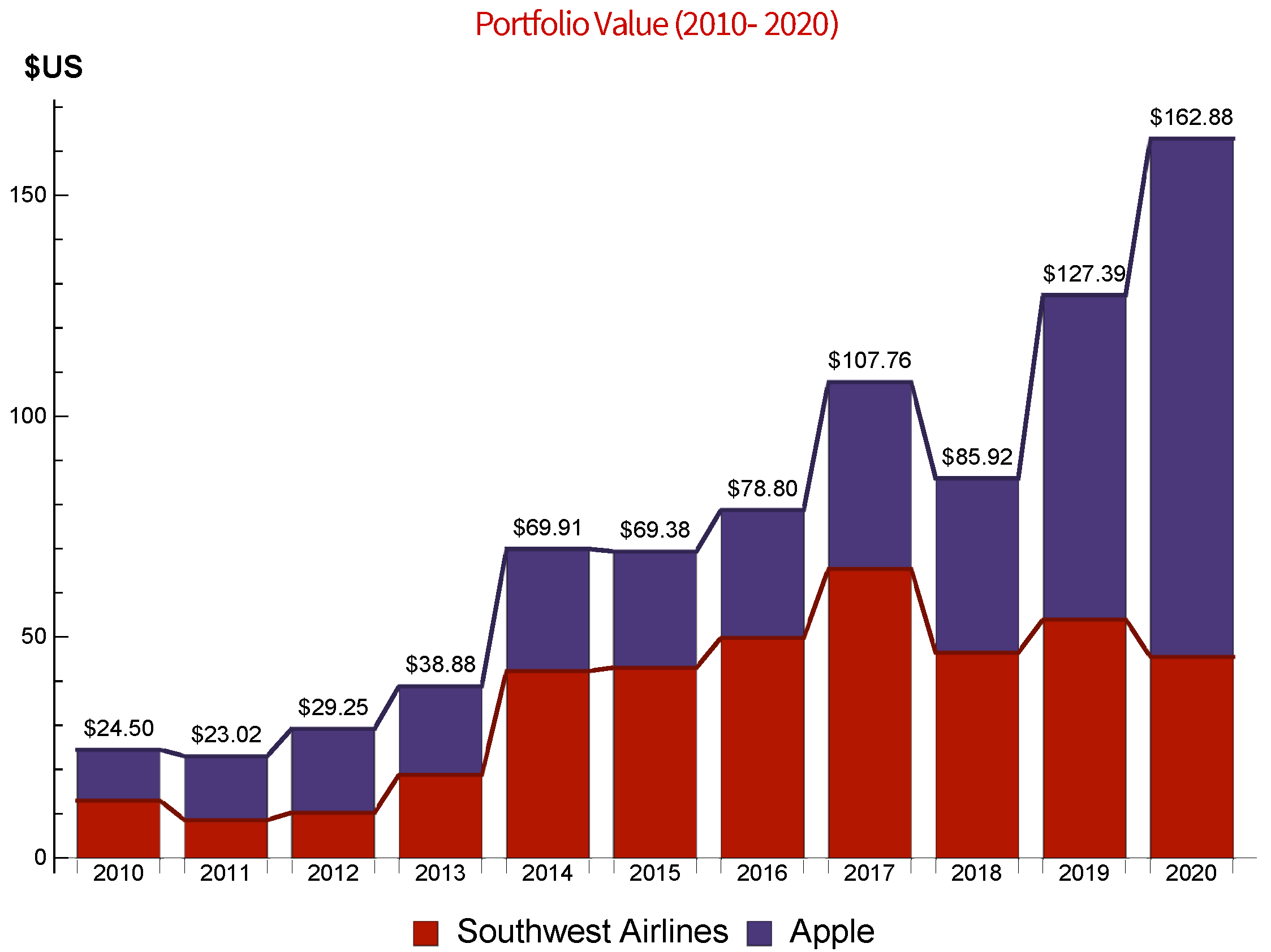
Southwest Airlines	NYSE:LUV	NYSE	Airlines	590273067	1 January 2015 through 31 December 2019	4 January 2020 through 20 November 2020
Apple	NASDAQ:AAPL	NASDAQ	Consumer Electronics	17001802000	1 January 2015 through 31 December 2019	4 January 2020 through 20 November 2020

. This is only one sample choice; in practice, any two highly correlated stocks inside a portfolio can be considered. The pairs can be obtained via strategies such as clustering analysis.

To show how the compared two stocks in our portfolio of companies behave through time, we compared their price trends, as shown in Figure 1.

Based on the discussions in Section 1, Section 2 and Section 3, it is now possible to write Algorithm 1 to perform the trading method. In fact, after constructing the copula function, the joint probability for each observed pair can be calculated.

Note that if only one joint distribution shows a lower tail dependence, then it is considered riskier than the one with a symmetric and weaker dependence.

The third item in Algorithm 1 includes a distribution fit test based on a hypothesis for test data. To illustrate the applicability of the proposed Laplace distribution in contrast to the normal distribution,

Table 2. Examination of whether the financial data follow the normal test under the best-fitted normal distribution. Goodness-of-fit tests are based on several well known statistical measures to test whether the sample data have the skewness and kurtosis matching a normal distribution.

	NYSE:LUV		NASDAQ:AAPL
Statistical Test	Statistic	p-Value	Statistic	p-Value
Pearson ${\chi }^2$	121.37	9.61 × 10${}^{-12}$	144.16	1.60 × 10${}^{-15}$
Cramér-von Mises	2.12	6.75 × 10${}^{-6}$	2.47	1.09 × 10${}^{-6}$
Anderson-Darling	12.23	1.82 × 10${}^{-6}$	14.21	6.50 × 10${}^{-7}$
Baringhaus-Henze	17.12	1.27 × 10${}^{-9}$	21.01	1.21 × 10${}^{-10}$
Jarque-Bera ALM	1510.45	0.	896.42	0.
Mardia Combined	1510.45	0.	896.42	0.
Mardia Kurtosis	37.95	2.86 × 10${}^{-315}$	29.25	3.64 × 10${}^{-188}$
Mardia Skewness	49.46	2.02 × 10${}^{-12}$	27.98	1.22 × 10${}^{-7}$
Shapiro–Wilk	0.94	1.46 × 10${}^{-21}$	0.94	2.67 × 10${}^{-20}$

and

Table 3. Examination of whether the financial data follow the best-fitted Laplace distribution.

	NYSE:LUV		NASDAQ:AAPL
Statistical Test	Statistic	p-Value	Statistic	p-Value
Pearson ${\chi }^2$	34.20	0.45	48.14	0.05
Cramér-von Mises	0.10	0.58	0.19	0.27
Anderson-Darling	0.67	0.57	1.10	0.30

are furnished based on the same test stocks we considered in Table 1. Floating shares are given based on the time of gathering the information for this work. The results clearly reveal that the normal distribution must not be assumed for the returns.

Several statistical test are shown in Table 2 and Table 3. Note that a statistical hypothesis test is a method of statistical inference used to determine a possible conclusion from two different, and likely conflicting, hypotheses [18] (Chapter 9). For instance, the Anderson-Darling test is a statistical test, which shows whether a considered set of data is drawn from a given probability distribution or not. In its basic form, the test assumes that there are no parameters to be estimated in the distribution being tested, in which case the test and its set of critical values is distribution-free. When applied to testing whether a normal distribution properly describes a set of data, it is one of the most useful tools in finding departures from normality.

At the sixth step of the Algorithm 1, one is able to derive a Gaussian copula with marginal Laplace distributions. The PDF of the constructed copula is plotted in Figure 2.

Algorithm 1 Pairs trade employing the Laplace marginal distribution function.

1: Choose the appropriate equity pair. Here, it was selected based on Table 1 on the given dates. 2: Gather daily prices on these indices and compute the log returns series. 3: Using the returns, we find the marginal distribution function. Here, the Laplace distribution based on Section 2 is fitted to these data. 4: We estimate the involved parameters by the maximum likelihood method. 5: The goodness-of-fit test is conducted and supports the selection of the Laplace distribution in contrast to the normal distribution with has a tighter tail dependency for the marginal distribution. This is where the proposed Laplace distribution helps us in practice. 6: Construct the bivariate normal copula (4), and save the final (estimated) copula distribution function as $\mathcal{D}$. 7: We calculate the returns during the out-of-sample period for our indices. 8: By considering the transactions costs to be negligible, we choose a threshold probability level of 95% and consider that we hold the trade for one day only, opening and closing the trade at the start and end of the day, after the signal is obtained. 9: Calculate each pair’s probability for daily observations. 10: Now, we obtain the signal based on the joint probabilities over the out-of-sample days of the series. 11: In the following days, when one observes the pairs with abnormally low/high estimated probabilities, s/he conducts the trading.

5. Simulation Results

In this work, the implementations were conducted using Mathematica 12.0 [19] (Chapter 7) with a computer equipped with Core i7-9750H and SSD memory. It is necessary to check the effectiveness of the derived Gaussian copula under the marginal Laplace distribution. For this purpose, in Figure 3, the empirical data of the two stocks are compared with ${10}^3$ random numbers generated using the Gaussian copula function with the fitted marginal Laplace distribution. The results show how well the revisited copula works for fitting financial data. This distribution is fits stock market returns better, and it allows professionals working in the industry to obtain a more realistic expectation of daily returns.

In

Table 4. Correlation comparisons for the considered sticks, as well as their lower and upper tails.

	Pearson	Spearman	Kendall
Overall	0.380776	0.360071	0.250801
Lower 5%-tile	0.375530	0.438191	0.323109
Upper 95%-tile	0.349495	0.333201	0.230797

, the Pearson correlation, the Spearman $\rho$, and the Kendall $\tau$ for all data as well as for the lower and upper tails of the distribution of stock returns are provided.

Recall that the key element needed for this strategy is a conditional probability function. In fact, $P(U\le u|V=v)$ and $P(V\le v|U=u)$ are differentiations of the associated copula in terms of v and u, respectively, (see for instance [5,20]:)

$$P\left(U\le u|V=v\right)=\frac{\partial C(u,v)}{\partial v},$$

(8)

$$P\left(V\le v|U=u\right)=\frac{\partial C(u,v)}{\partial u}.$$

(9)

Note that the probability threshold is always an obstacle for this approach. However, stocks are determined as being relatively undervalued as long as the conditional probability is less than 0.5 and relatively overvalued as long as the conditional probability is greater than 0.5 [20]. Additionally, the conditional probabilities’ values are an indication of the certainty or confidence about the position of the stocks as well.

Thus, the execution of trade must be performed when one of the conditional probabilities is approaching 1. As such, the use of conditional probability functions is necessary for the strategy.

Some of the results are shown in

Table 5. Results based on pairs trade and Algorithm 1 showing when to conduct the trades based on the probabilities.

	NYSE:LUV	NASDAQ:AAPL	Probability
6 January 2020	0.01580	0.02255	0.02
7 January 2020	−0.00897	−0.00976	0.65
8 January 2020	−0.00405	0.00793	0.20
9 January 2020	0.00295	−0.00471	0.33
10 January 2020	0.00147	0.01595	0.08
13 January 2020	−0.00128	0.02101	0.06
14 January 2020	−0.00665	0.00225	0.35
15 January 2020	0.00092	0.02113	0.05
16 January 2020	0.00921	−0.01359	0.23
17 January 2020	0.00986	−0.00429	0.19
21 January 2020	0.00489	0.01248	0.09
22 January 2020	−0.00525	0.01101	0.16
23 January 2020	−0.02708	−0.00679	0.72
24 January 2020	−0.00112	0.00356	0.26
27 January 2020	0.03527	0.00480	0.01
28 January 2020	0.02054	−0.00288	0.08
29 January 2020	−0.00531	−0.02984	0.67
30 January 2020	0.02371	0.02789	0.009
31 January 2020	−0.01240	0.02071	0.07
3 February 2020	−0.01880	−0.00145	0.55
4 February 2020	−0.01534	−0.04535	0.85
5 February 2020	0.00435	−0.00275	0.28
6 February 2020	0.00829	0.03248	0.01
7 February 2020	0.02255	0.00812	0.04
10 February 2020	0.01343	0.01162	0.05
11 February 2020	−0.00800	−0.01605	0.69
12 February 2020	0.00279	0.00473	0.19
13 February 2020	0.00884	−0.00605	0.21
14 February 2020	0.00944	0.02347	0.03
18 February 2020	0.00102	−0.00714	0.40
19 February 2020	−0.00978	0.00024	0.44
20 February 2020	−0.00640	−0.01848	0.67
21 February 2020	−0.00854	0.01437	0.13
24 February 2020	−0.00298	−0.01031	0.54
25 February 2020	−0.00722	−0.02289	0.70
26 February 2020	−0.04375	−0.04866	0.98
27 February 2020	−0.08581	−0.03445	0.97
28 February 2020	−0.01542	0.01573	0.12
2 March 2020	−0.04753	−0.06760	0.98
3 March 2020	−0.00948	−0.00058	0.47

for pairs trading. After a very high probability reading for 26 February 2020, we can conduct the trading. To illustrate further, we see the very high probability; then, by taking equal weighted positions, we long the NASDAQ:AAPL index and short the NYSE:LUV index on 27 February 2020. We close the position at the end of the day, producing a total return of 5.136%. Similarly, we can employ this pairs trade method to the entire sample and illustrate the resulting profit and loss.

Further acceleration of the pairs trade under Laplace marginal distribution can be pursued using parallel computation. In fact, using parallelization of the $\mathtt{Table}\left[\right]$ Mathematica command or the similar ones used in programming can help to improve the CPU time of the running times as much as possible.

In sum, the computational pieces of evidence reveal that the pairs trading under a copula approach is a good choice as long as a fat-tail marginal distribution (such as the Laplace distribution) is employed for fitting the data when we are calibrating the copula function.

6. Conclusions

In this paper, we reviewed pairs trading using the copula approach with an emphasis on the use of the well-known fat-tailed Laplace distribution. The fat-tailed feature of the considered distribution, particularly when used on the marginal functions, helped us to produce copula distribution functions, which had a better ability to fit stock data. The computational pieces of evidence in Section 5 supported the discussions.

Finally, we note that due to the growth in the availability of data, sometimes it is difficult to determine efficient pairs. Hence, further questions can be investigated in future studies such as:

• How to determine the best pairs while limiting the search space; and,
• How to stop facing long decline periods due to prolonged divergent pairs.

References

- Basel Committee on Banking Supervision. Basel III: A Global Regulatory Framework for More Resilient Banks and Banking Systems; Basel Committee on Banking Supervision: Basel, Switzerland, 2011. [Google Scholar]
- Company, R.; Egorova, V.N.; Jódar, L.; Soleymani, F. A stable local radial basis function method for option pricing problem under the Bates model. Numer. Methods Part. Differ. Equ. 2019, 35, 1035–1055. [Google Scholar] [CrossRef]
- Tsoulos, I.G.; Kosmas, O.T.; Stavrou, V.N. DiracSolver: A tool for solving the Dirac equation. Comput. Phys. Commun. 2019, 236, 237–243. [Google Scholar] [CrossRef] [Green Version]
- Alexander, C. Market Risk Analysis, Chichester; John Wiley & Sons Ltd.: West Sussex, UK, 2008. [Google Scholar]
- Kinlay, J. Pairs Trading with Copulas. 2019, pp. 1–9. Available online: community.wolfram.com (accessed on 26 January 2022).
- Maneejuk, P.; Yamaka, W. The role of economic contagion in the inward investment of emerging economies: The dynamic conditional copula approach. Mathematics 2021, 9, 2540. [Google Scholar] [CrossRef]
- Sklar, A. Fonctions de répartition à n dimension et leurs marges. Publ. L’Institut Stat. L’Université Paris 1959, 8, 229–231. [Google Scholar]
- Okhrin, O.; Ristig, A.; Xu, Y.-F. Copulae in High Dimensions: An Introduction. Appl. Quant. Financ. Stat. Comput. 2017, 13, 247–277. [Google Scholar]
- Gerlach, R.; Lu, Z.; Huang, H. Exponentially smoothing the skewed Laplace distribution for value-at-risk forecasting. J. Forecast. 2013, 32, 534–550. [Google Scholar] [CrossRef]
- Ghanadian, A.; Lotfi, T. Approximate solution of nonlinear Black-Scholes equation via a fully discretized fourth-order method. AIMS Math. 2020, 5, 879–893. [Google Scholar] [CrossRef]
- Itkin, A.; Soleymani, F. Four-factor model of quanto CDS with jumps-at-default and stochastic recovery. J. Comput. Sci. 2021, 54, 101434. [Google Scholar] [CrossRef]
- Ernst, P.A.; Soleymani, F. A Legendre-based computational method for solving a class of Itô stochastic delay differential equations. Numer. Algorithms 2019, 80, 1267–1282. [Google Scholar] [CrossRef]
- Kotz, S.; Kozubowski, T.J.; Podgórski, K. The Laplace Distribution and Generalizations: A Revisit with Applications to Communications, Economics, Engineering and Finance; Birkhauser: Basel, Switzerland, 2001. [Google Scholar]
- Taylor, J. Forecasting value at risk and expected shortfall using a semiparametric approach based on the asymmetric Laplace distribution. J. Bus. Econ. Stat. 2019, 37, 121–133. [Google Scholar] [CrossRef]
- Blázquez, M.C.; De la Cruz, C.D.O.; Román, C.P. Pairs trading techniques: An empirical contrast. Eur. Res. Manag. Bus. Econ. 2018, 24, 160–167. [Google Scholar] [CrossRef]
- Do, B.; Faff, R. Does simple pairs trading still work? Finan. Anal. J. 2010, 66, 83–95. [Google Scholar] [CrossRef]
- Soleymani, F.; Vasighi, M. Efficient portfolio construction by means of CVaR and k-means++ clustering analysis: Evidence from the NYSE. Int. J. Finan. Econ. 2021, 1–15. [Google Scholar] [CrossRef]
- Rice, J.A. Mathematical Statistics and Data Analysis, 3rd ed.; Thomson Brooks/Cole.: Belmont, CA, USA, 2007. [Google Scholar]
- Georgakopoulos, N.L. Illustrating Finance Policy with Mathematica; Springer International Publishing: Cham, Switzerland, 2018. [Google Scholar]
- Liew, R.Q.; Wu, Y. Pairs trading: A copula approach. J. Deriv. Hedge Funds 2013, 19, 12–30. [Google Scholar] [CrossRef] [Green Version]