Stability Analysis and Synthesis for 2-D Switched Systems with Random Disturbance

Abstract

In this paper, the stability analysis and controller design of two-dimensional (2-D) switched system with random disturbances are studied. First, based on the Fornasini–Marchesini local state space model, a random discrete 2-D switched system model is proposed. Secondly, based on the method of switching quadratic Lyapunov function, Schur complement and linear matrix inequality the criterion of the sufficiency of the asymptotically stable under any switching signal is established. The extended average residence time method is used to obtain a sufficient criterion of the mean square exponential stability of the random discrete 2-D switched system under restricted switching conditions. According to the stability analysis results, the conditions for the existence of the state feedback controller are given and the corresponding state feedback controller is designed. Finally, two examples are given to illustrate the effectiveness of the proposed method.

1. Introduction

In recent decades, many researchers have received significant attention from the related theoretical research of 2-D systems. The difference from 1- to 2-D systems is that the dynamic process of 2-D systems depends on two interdependent variables. Therefore, 2-D systems can be applied to many actual system modelling, such as digital filters, signal processing, image enhancement [1], etc. Discrete-time 2-D systems have gradually become an important research direction of 2-D systems with the rapid development of science and technology. It can be seen in [2,3,4], the stability analysis problem of the 2-D system has been solved. In [5], Gao studied the stability and $H_{\infty }$ control of a 2-D system with Markov jump parameters. For the 2-D linear uncertain time-varying system, Dong et al. [6] introduced an alternative indefinite quadratic performance function to replace the standard $H_{\infty }$ performance index.

The switched system is a typical hybrid hopping system [7]. A switched system is a dynamic system composed of several subsystems and switching signals that control the switching between the subsystems. The switched systems can describe its model with less complicated mathematical expressions, and the constructed model can be in good agreement with the actual situation. An interesting phenomenon of the switched system is that even if all subsystems are unstable if the switching signal is properly designed between unstable modes, the switched system can be asymptotically stable [8,9]. Zhu [10] investigates the region stabilization issue of switched neural networks (SNNs) with multiple modes (MMs) and multiple equilibria (ME) via a pole assignment method. Note that the participation of switching signals will lead to quantitative behaviour and have a certain impact on system performance. For example, even if all subsystems are unstable, the stability of the discrete-time switched system can be guaranteed by appropriate switching signals. In [11], sufficient conditions for the magnitude of delay for switched nonlinear systems with external disturbances are given, which guarantees the global exponential stability of switched systems.

Like the 1-D systems, the actual 2-D systems often has sudden changes or failures, and it can be modelled as a 2-D switched system. Because the 2-D switched system integrates the complex internal structure characteristics of all the subsystems of the 2-D systems and the problematic dynamic behaviour induced by the switching signal, its research is precious. In [12,13], Benzaouia et al. studied the stability analysis and customization of the 2-D switched systems, and there are some preliminary results. In [14], the stabilization problem of 2-D switched systems represented by the FM local state space model and the Roesser model is addressed by switching signal conditioning. In [15], for discrete-time 2-D switched systems, a quasi-time-varying (QTD) $H_{\infty }$ filtering method is proposed to ensure that the filtering error system is exponentially stable. Gao [16] et al. further analyzed the weighted robust $H_{\infty }$ interference attenuation performance of the underlying system. Ren et al. [17] designed a 2-D stationary discrete-time linear filter with a specified $H_{\infty }$ performance for all admissible uncertain parameters. Recently, Badie et al. [18] studied the problem of time-delay-dependent exponential stability analysis of 2-D discrete switched systems with time-varying delays described by the Roesser model. Kaiqun et al. [19] studied the single-point control and external disturbance problems of 2-D switched systems on the basis of nominal system information compensation.

To date, stability analysis and switching stability are still the main concerns switched systems. Stability is one of the basic concepts of the control system and plays a critical role in the design of the control system. In this paper, there are roughly two types of stability issues:

1.

System stability without being restricted by switching signals:

The switching signal does not restrict the 2-D switched systems. Even if every subsystem in the system is in a stable state, the entire 2-D switched system may be unstable under a specific switching signal.

2.

System stability under restricted switching laws:

The switched system may not be stable under arbitrary switching, but the system may be stable under restricted switching signals, such as a closed-loop multi-controller system. Dwell time and average dwell time switching are typical restricted switching signals. They were proposed and developed by Hespanha and Morse [20,21,22], respectively. Applying it to a restricted switching signal can effectively solve the stability problem in restricted switching.

Most switching rules are divided into two categories for switched systems: random, such as Markov jumping system; deterministic, such as time and state-related switching rules. In recent years, 1-D systems with random disturbances have received widespread attention in various fields, and many basic results of deterministic systems have been extended to random situations. For the actual 2-D systems, external interference is often inevitable, which will seriously deteriorate the control performance of the system. Random phenomena appear widely in fields such as system science, engineering control and finance. Therefore, in many branches of science, random modelling occupies a significant position, and systems subject to random disturbances have gradually attracted the attention of scholars. In particular, in [23,24], $H_2/H_{\infty }$ control and output feedback stabilization with multiplicative noise are studied. The stochastic stability and $H_{\infty }$ control of a 2-D continuous time-delay Markov jump system with partial transition probability information are studied in [25]. In [26], the time-varying problem of semi-Markov jumping linear systems (S-MJLSs) is fully considered, and sufficient conditions are given to check the stochastic stability of the underlying system.

For 2-D systems, the analysis and design problems become more complex and challenging than normal systems because the random signal is multiplied by the relevant system state. Many methods and results about the stability, performance analysis and controller synthesis of random multiplicative noise dynamic systems have been reported in the literature. For the first time in reference [5], the 2-D discrete linear system with random disturbances was considered. Then they considered the robustness of the proposed system in reference [27]. Yao et al. [28] considered the influence of state lag on 2-D discrete stochastic systems, and studied the robust control of the system in this case. In [29,30], the stability analysis and state estimation of the 2-D discrete system coefficient matrix are considered when subjected to the random disturbance. In [31], the 2-D switched system under arbitrary and restricted conditions is studied. However, few people will analyze and synthesize a 2-D random switched system whose system matrix is randomly disturbed.

Inspired by the above introduction, this paper will study the stability analysis, and controller design of a class of 2-D switched systems with random disturbance under arbitrary and restricted switching conditions. First, a random discrete 2-D switched system model is established based on the Fornasini–Marchesini local state space (FMLSS) model. The mean square asymptotic stability and the mean square exponential stability of the switched system under arbitrary and restricted switching, the random discrete 2-D switched system is derived through linear matrix inequality (LMI) technology. On this basis, the sufficient LMI conditions of the state feedback controller are obtained and verified by practical numerical algorithms.

The rest of this article is organized as follows. The issues considered are explained in Section 2. Section 3 gives the conditions for the stability of the 2-D switched system under arbitrary and restricted switching signals. According to the results of Section 3, the design method of stabilization controller is given in Section 4. Section 5 provides an example to verify the effectiveness of the proposed method, and concludes this article in Section 6.

Notation: Our notations are fairly standard. Symbols used in the paper: superscript T represents matrix transposition; $R^n$ represents n-dimensional Euclidean space; $R^{m\times n}$ is the set of all real matrices of $m\times n$ dimension, symbol $P>0$ represents P is real symmetric positive definite; I and 0 represent units Matrix and zero matrix; $∥•∥$ refers to the Euclidean vector norm; ${\lambda }_{min}\left(•\right)$ and ${\lambda }_{max}\left(•\right)$ represent the minimum eigenvalue and maximum eigenvalue of the matrix, respectively. Function $ceil\left(a\right)$ represents rounding real number a to the nearest integer greater than or equal to a. In the block symmetric matrix or long matrix expression, we use an asterisk $“\ast ”$ to indicate symmetry, and $diag\left\{\cdots \right\}$ to indicate a block diagonal matrix.

2. Problem Formulation

The discrete-time 2-D system described by the FMLSS model (Kaczorek, 1985):

$$x_{i+1,j+1}=A_1{x}_{i,j+1}+A_2{x}_{i+1,j}+B_1{u}_{i,j+1}+B_2{u}_{i+1,j}$$

(1)

where $x_{i,j}\in R^n$ is the local state vector; $u_{i,j}\in R^n$ is the input, $(i,j)\in N\times N$; $A_1,A_2,B_1,B_2$ is the known system matrix, and the sequence $x_{0,j},x_{i,0}$ represents the initial conditions.

Remark 1.

Because the Fornasini–Marchesini (FM) model is more general, usually Attasi model and Roesser model can be considered as special cases. Therefore, we chose to consider the stability analysis and stabilization of the more general FM-type 2-D switched system.

Definition 1.

($\epsilon -\delta$ Stability) System (1) is said to be stable in the sense of Lyapunov under the zero input ${\mathit{u}}_{i,j}=0$ if $\forall \epsilon >0$, there exists $\delta \left(\epsilon \right)>0$ such that if $\parallel x_{0,j}\parallel <\delta$, $\parallel x_{i,0}\parallel <\delta$ then $\parallel x_{i,j}\parallel <\epsilon ,\forall i,j>0$.

Definition 2.

(Asymptotic stability) If the system (1) is asymptotically stable, it satisfies: Lyapunov stability and when the time t tends to infinity, the state trajectory tends to balance. In this article, when $\underset{j\to \infty }{lim}\left|\right|x_{0,j}\left|\right|=0,\underset{i\to \infty }{lim}\left|\right|x_{i,0}\left|\right|=0$, we have $\underset{i+j\to \infty }{lim}\left|\right|x_{i,j}\left|\right|=0$.

Remark 2.

Yeganefar et al. [31] proposed the definition of asymptotic stability and exponential stability of discrete-time 2-D systems, and proposed two different Lyapunov theorems to test these definitions. If the 2-D system (1) is asymptotically stable, the $\epsilon -\delta$ stable condition is first met. Unlike the 1-D system, the initial conditions do not need to be zero at infinity.

Assumption 1.

Assume that the following initial conditions are satisfied:

$$\underset{\Gamma \to \infty }{lim}\sum _{i=0}^{\Gamma }\left(\right|\left|x_{i,0}\right|{|}^2+\left|\right|x_{0,i}\left|{|}^2\right)<\infty$$

(2)

Remark 3.

There is no doubt that the above assumption satisfies $\underset{j\to \infty }{lim}\left|\right|x_{0,j}\left|\right|=0,\underset{i\to \infty }{lim}\left|\right|x_{i,0}\left|\right|=0$. If the system is gradually stable, just prove $\underset{i+j\to \infty }{lim}\left|\right|x_{i,j}\left|\right|=0$.

With the rapid development of control technology, in the design of feedback control systems today, it is often necessary to consider the systems with random disturbance, that is, the robustness of the system. When dealing with many robust control problems of this systems and many other control problems caused by control system theory, they can be transformed into a kind of linear matrix inequality or a problem with linear matrix inequality constraints. In control engineering theory, most control problems can be transformed into linear matrix inequality problems.

Lemma 1.

If there is a matrix $P>0$, and positive scalars α and β satisfy $\alpha +\beta =1$ such that:

$${\overline{A}}^{T}P\overline{A}-Q<0$$

(3)

where

$$\overline{A}\stackrel{\Delta }{=}\left[A_1,A_2\right],\overline{Q}\stackrel{\Delta }{=}\left[\begin{array}{cc}\alpha P& 0\\ 0& \beta P\end{array}\right].$$

Then the 2-D discrete system in (1) is asymptotically stable under zero input.

Lemma 2.

The 2-D discrete-time system in (1) under the zero input is asymptotically stable if there exist matrices $P>0$ and $Q>0$ such that:

$$\left[\begin{array}{cc}{A}_1^{T}P{A}_1+Q-P& *\\ A_2^{T}P{A}_1& A_2^{T}P{A}_2-Q\end{array}\right]<0$$

(4)

Lemma 3.

The following three results are equivalent, if there is a symmetric matrix $S=\left[\begin{array}{cc}{S}_{11}& S_{12}\\ S_{12}^T& S_{22}\end{array}\right]$, where $S_{11}\in R^{r\times r}$:

1.

$S<0$

2.

$S_{11}<0$ and $S_{22}-S_{12}^T{S}_{11}^{-1}{S}_{12}<0$

3.

$S_{12}<0$ and $S_{11}-S_{12}^T{S}_{22}^{-1}{S}_{12}<0$

After the above discussion, we consider the mean square asymptotic stability of a 2-D discrete random system and define it as follows:

Definition 3.

If $u_{i,j}=0$ under zero input and for each initial condition $E\left\{{\left|x_{i,j}\right|}^2\right\}<\infty$, then the 2-D discrete random system under (1) is asymptotically stable in mean square.

$$\underset{i+j\to \infty }{lim}E\left\{{\left|x_{i,j}\right|}^2\right\}=0$$

(5)

Definition 4.

If the constants $\eta >0$ and $0<\rho <1$, the system is exponentially stable in mean square under the switching signal α, then the solution of system (1) satisfies:

$$\sum _{i+j=\Gamma }E\left\{{∥x_{i,j}∥}^2\right\}\le \eta {\rho }^{\Gamma -k_0}\sum _{i+j=k_0}E\{{∥x_{i,j}∥}^2\}$$

(6)

Similar to the well-established discrete-time switched model of 1-D system, we consider the following discrete-time 2-D switched model:

$$\begin{array}{c}\hfill x_{i+1,j+1}=A_1\left({\alpha }_{i,j+1}\right)x_{i,j+1}+A_2\left({\alpha }_{i+1,j}\right)x_{i+1,j}\\ \hfill +B_1\left({\alpha }_{i,j+1}\right)u_{i,j+1}+B_2\left({\alpha }_{i+1,j}\right)u_{i+1,j}\end{array}$$

(7)

where ${\alpha }_{i,j}$ is a switching signal; $(A_1\left({\alpha }_{i,j+1}\right),A_2\left({\alpha }_{i+1,j}\right),B_1\left({\alpha }_{i,j+1}\right),B_2\left({\alpha }_{i+1,j}\right):{\alpha }_{i,j+1}={\alpha }_{i+1,j}\in N)$ is a family of matrices parameterized by an index set N. When ${\alpha }_{i,j}=l\in N$, $A_1\left({\alpha }_{i,j}\right)=A_1\left(l\right)$ and $A_2\left({\alpha }_{i,j}\right)=A_2\left(l\right)$. The boundary condition is also assumed to satisfy Assumption 1. Therefore, the 2-D switched system effectively switches amongst N subsystems with the switching sequence controlled by ${\alpha }_{i,j}$. We assume that the value of ${\alpha }_{i,j}$ is unknown a prior, but its instantaneous value is available in real time. So, we consider the following 2-D discrete stochastic switched system:

$$\begin{array}{c}{x}_{i+1,j+1}=\left[A_1\left({\alpha }_{i,j+1}\right)x_{i,j+1}+A_2\left({\alpha }_{i+1,j}\right)x_{i+1,j}\right]\hfill \\ \begin{array}{cccc}& & & \end{array}+\left[M_1\left({\alpha }_{i,j+1}\right)x_{i,j+1}+M_2\left({\alpha }_{i+1,j}\right)x_{i+1,j}\right]v_{i,j}\hfill \\ \begin{array}{cccc}& & & \end{array}+B_1\left({\alpha }_{i,j+1}\right)u_{i,j+1}+B_2\left({\alpha }_{i+1,j}\right)u_{i+1,j}\hfill \end{array}$$

(8)

where $M_1$, $M_2$ is a matrix of appropriate size, $v_{i,j}$ is independent 2-D random variables with zero mean satisfying:

$$\left\{\begin{array}{c}E\left\{v_{i,j}{v}_{m,n}\right\}=1if(i,j)=(m,n)\\ E\left\{v_{i,j}{v}_{m,n}\right\}=0if(i,j)\ne (m,n)\end{array}\right.$$

(9)

The stochastic signal $v_{i,j}$ for 2-D discrete-time systems has been introduced in [30].

Rewrite system S in the following form:

$$\begin{array}{c}{x}_{i+1,j+1}=\left[A_1\left({\alpha }_{i,j+1}\right)+M_1\left({\alpha }_{i,j+1}\right)v_{i,j}\right]x_{i,j+1}\hfill \\ \begin{array}{cccc}& & & \end{array}+\left[A_2\left({\alpha }_{i+1,j}\right)+M_2\left({\alpha }_{i+1,j}\right)v_{i,j}\right]x_{i+1,j}\hfill \\ \begin{array}{cccc}& & & \end{array}+B_1\left({\alpha }_{i,j+1}\right)u_{i,j+1}+B_2\left({\alpha }_{i+1,j}\right)u_{i+1,j}\hfill \end{array}$$

(10)

We can see that the terms $M_1\left({\alpha }_{i,j+1}\right)v_{i,j}$ and $M_2\left({\alpha }_{i+1,j}\right)v_{i,j}$ can be seen as stochastic perturbations to the system matrices $A_1\left({\alpha }_{i,j+1}\right)$ and $A_2\left({\alpha }_{i+1,j}\right)$, respectively.

3. Stability Analysis with Random Disturbance

3.1. Under Arbitrary Switching

In order to establish the stability of the system, we first assume $u_{i,j}=0$, and then express the open-loop model of the system as:

$$\begin{array}{c}\hfill \begin{array}{c}{x}_{i+1,j+1}=\left[A_1\left({\alpha }_{i,j+1}\right)x_{i,j+1}+A_2\left({\alpha }_{i+1,j}\right)x_{i+1,j}\right]\hfill \\ \begin{array}{ccc}\begin{array}{cc}& \end{array}& & \end{array}+\left[M_1\left({\alpha }_{i,j+1}\right)x_{i,j+1}+M_2\left({\alpha }_{i+1,j}\right)x_{i+1,j}\right]v_{i,j}\hfill \\ \begin{array}{cc}& \begin{array}{cc}& \end{array}\end{array}=\left[A_1\left({\alpha }_{i,j+1}\right)+M_1\left({\alpha }_{i,j+1}\right)v_{i,j}\right]x_{i,j+1}\hfill \\ \begin{array}{ccc}& & \begin{array}{cc}& \end{array}\end{array}+\left[A_2\left({\alpha }_{i+1,j}\right)+M_2\left({\alpha }_{i+1,j}\right)v_{i,j}\right]x_{i+1,j}\hfill \end{array}\end{array}$$

(11)

where ${\alpha }_{i,j}:(Z^{+},Z^{+})\to N$ is a piecewise constant function of time, called a switching signal, which takes its values in the finite set $N\left\{1,2,\dots ,N\right\}$, where N is the number of subsystems; $\left\{A_1\left({\alpha }_{i,j+1}\right),A_2\left({\alpha }_{i+1,j}\right),B_1\left({\alpha }_{i,j+1}\right),B_2\left({\alpha }_{i+1,j}\right):{\alpha }_{i,j+1}={\alpha }_{i+1,j}\in N\right\}$ is a family of matrices parameterized by an index set N. $M_1$, $M_2$ is a matrix of appropriate size, $v_{i,j}$ is independent 2-D random variables.

Next, we will focus on analyzing the stability of the 2-D switched system under arbitrary switching signals.

First, the arbitrary switching is discussed. The following theorem gives a sufficient condition for the discrete-time 2-D switched system to be asymptotically stable under arbitrary switching signals.

Theorem 1.

The discrete-time 2-D switched system (8) is asymptotically stable if there exist matrices $P\left(l\right)>0$, $P\left(k\right)>0$ and $Q\left(k\right)>0$, $\forall k,l\in N$ such that the following linear matrix inequality(LMI) holds:

$$\begin{array}{c}\left[\begin{array}{cc}-P\left(k\right)+Q\left(k\right)& 0\\ *& -Q\left(k\right)\\ *& *\\ *& *\end{array}\right.\hfill \\ \left.\begin{array}{cc}{A_1}^T\left(k\right)P\left(l\right)& {A_1}^T\left(k\right)P\left(l\right)\\ {A_2}^T\left(k\right)P\left(l\right)& {M_2}^T\left(k\right)P\left(l\right)\\ -P\left(l\right)& 0\\ *& -P\left(l\right)\end{array}\right]<0\end{array}$$

Proof. 

To establish the stability of the discrete-time 2-D switched system, we consider the following index:

$$\begin{array}{c}\hfill \begin{array}{c}\zeta \stackrel{\Delta }{=}E\{x_{i+1,j+1}^{T}P\left({\alpha }_{i+1,j+1}\right)x_{i+1,j+1}\left|\tilde{x}\}\right.\hfill \\ \begin{array}{cc}& \end{array}-x_{i,j+1}^T[P\left({\alpha }_{i,j+1}\right)-Q\left({\alpha }_{i,j+1}\right)]x_{i,j+1}\hfill \\ \begin{array}{cc}& \end{array}-x_{i+1}^{T}Q\left({\alpha }_{i+1,j}\right)x_{i+1,j}\hfill \\ =E\left\{\left.\left\{\begin{array}{c}\left(\begin{array}{c}{\left(\begin{array}{c}\left[\begin{array}{c}{A}_1\left({\alpha }_{i,j+1}\right)x_{i,j+1}\hfill \\ +A_2\left({\alpha }_{i+1,j}\right)x_{i+1,j}\hfill \end{array}\right]\hfill \\ +\left[\begin{array}{c}{M}_1\left({\alpha }_{i,j+1}\right)x_{i,j+1}\hfill \\ +M_2\left({\alpha }_{i+1,j}\right)x_{i+1,j}\hfill \end{array}\right]{\nu }_{i,j}\hfill \end{array}\right)}^T\hfill \\ P\left({\alpha }_{i+1,j+1}\right)\hfill \end{array}\right)\hfill \\ \times \left(\begin{array}{c}\left[\begin{array}{c}{A}_1\left({\alpha }_{i,j+1}\right)x_{i,j+1}\hfill \\ +A_2\left({\alpha }_{i+1,j}\right)x_{i+1,j}\hfill \end{array}\right]\hfill \\ +\left[\begin{array}{c}{M}_1\left({\alpha }_{i,j+1}\right)x_{i,j+1}\hfill \\ +M_2\left({\alpha }_{i+1,j}\right)x_{i+1,j}\hfill \end{array}\right]{\nu }_{i,j}\hfill \end{array}\right)\hfill \end{array}\right\}\right|\tilde{x}\right\}\hfill \\ \begin{array}{cc}& \end{array}-x_{i,j+1}^T[P\left({\alpha }_{i,j+1}\right)-Q\left({\alpha }_{i,j+1}\right)]x_{i,j+1}\hfill \\ \begin{array}{cc}& \end{array}-x_{i+1}^{T}Q\left({\alpha }_{i+1,j}\right)x_{i+1,j}\hfill \\ ={\tilde{x}}^T\Psi \tilde{x}\hfill \end{array}\end{array}$$

(12)

where

$$\begin{array}{c}\Psi =\left[\begin{array}{cc}{\Psi }_{11}& {\Psi }_{12}\\ & {\Psi }_{22}\end{array}\right]\hfill \\ {\Psi }_{11}={M_1}^T\left({\alpha }_{i,j+1}\right)P\left({\alpha }_{i+1,j+1}\right)M_1\left({\alpha }_{i,j+1}\right)\hfill \\ \begin{array}{ccc}& & \end{array}+{A_1}^T\left({\alpha }_{i,j+1}\right)P\left({\alpha }_{i+1,j+1}\right)A_1\left({\alpha }_{i,j+1}\right)\hfill \\ \begin{array}{ccc}& & \end{array}-P\left({\alpha }_{i,j+1}\right)+Q\left({\alpha }_{i,j+1}\right)\hfill \\ {\Psi }_{12}={M_1}^T\left({\alpha }_{i,j+1}\right)P\left({\alpha }_{i+1,j+1}\right)M_2\left({\alpha }_{i+1,j}\right)\hfill \\ \begin{array}{ccc}& & \end{array}+{A_1}^T\left({\alpha }_{i,j+1}\right)P\left({\alpha }_{i+1,j+1}\right)A_2\left({\alpha }_{i+1,j}\right)\hfill \\ {\Psi }_{22}={M_2}^T\left({\alpha }_{i+1,j}\right)P\left({\alpha }_{i+1,j+1}\right)M_2\left({\alpha }_{i+1,j}\right)\hfill \\ \begin{array}{ccc}& & \end{array}+{A_2}^T\left({\alpha }_{i+1,j}\right)P\left({\alpha }_{i+1,j+1}\right)A_2\left({\alpha }_{i+1,j}\right)-Q\left({\alpha }_{i+1,j}\right)\hfill \end{array}$$

$$\tilde{x}\stackrel{\Delta }{=}\left[\begin{array}{c}{x}_{i,j+1}\\ x_{i+1,j}\end{array}\right]$$

(13)

From Theorem 1, we have $\Psi <0$, that is, $\varsigma <0$ for any $\tilde{x}\ne 0$. Therefore:

$$\begin{array}{c}\hfill \begin{array}{c}E\{x_{i+1,j+1}^{T}P\left({\alpha }_{i+1,j+1}\right)x_{i+1,j+1}\left|\tilde{x}\}\right.\hfill \\ \begin{array}{cc}& \end{array}<x_{i,j+1}^T[P\left({\alpha }_{i,j+1}\right)-Q\left({\alpha }_{i,j+1}\right)]x_{i,j+1}\hfill \\ \begin{array}{cc}& \begin{array}{cc}& \end{array}\end{array}+x_{i+1}^{T}Q\left({\alpha }_{i+1,j}\right)x_{i+1,j}\hfill \end{array}\end{array}$$

(14)

Take the expectation on both sides of the above formula:

$$\begin{array}{c}\hfill \begin{array}{c}E\left\{x_{i+1,j+1}^{T}P\left({\alpha }_{i+1,j+1}\right)x_{i+1,j+1}\right\}\hfill \\ \begin{array}{cc}& \end{array}<E\left\{x_{i,j+1}^T[P\left({\alpha }_{i,j+1}\right)-Q\left({\alpha }_{i,j+1}\right)]x_{i,j+1}\right\}\hfill \\ \begin{array}{ccc}& & \end{array}+E\left\{x_{i+1}^{T}Q\left({\alpha }_{i+1,j}\right)x_{i+1,j}\right\}\hfill \end{array}\end{array}$$

(15)

We can see that there is a variable $\delta \in \left(0,1\right)$, the (12) written as follows:

$$\begin{array}{c}\hfill \begin{array}{c}E\left\{x_{i+1,j+1}^{T}P\left({\alpha }_{i+1,j+1}\right)x_{i+1,j+1}\right\}<\hfill \\ \begin{array}{cc}& \end{array}\delta \left\{\begin{array}{c}E\left\{x_{i,j+1}^T[P\left({\alpha }_{i,j+1}\right)-Q\left({\alpha }_{i,j+1}\right)]x_{i,j+1}\right\}\hfill \\ +E\left\{x_{i+1}^{T}Q\left({\alpha }_{i+1,j}\right)x_{i+1,j}\right\}\hfill \end{array}\right\}\hfill \end{array}\end{array}$$

(16)

Note that Theorem 1 implies that $P\left({\alpha }_{i,j+1}\right)>Q\left({\alpha }_{i,j+1}\right)$, so

$$\begin{array}{c}\hfill \begin{array}{c}E\left\{x_{i+1,0}^{T}P\left({\alpha }_{i+1,0}\right)x_{i+1,0}\right\}=E\left\{x_{i+1,0}^{T}P\left({\alpha }_{i+1,0}\right)x_{i+1,0}\right\},\hfill \\ E\left\{x_{i,1}^{T}P\left({\alpha }_{i,1}\right)x_{i,1}^{}\right\}\hfill \\ \begin{array}{cccc}& & & \end{array}\le \delta E\left\{x_{i-1,1}^T\left[P\left({\alpha }_{i-1,1}\right)-Q\left({\alpha }_{i-1,1}\right)\right]x_{i-1,1}\right\}\hfill \\ \begin{array}{cccc}\begin{array}{cc}& \end{array}& & & \end{array}+\delta E\left\{x_{i,0}^{T}Q\left({\alpha }_{i,0}\right)x_{i,0}\right\}\hfill \\ \begin{array}{cccc}& & & \end{array}<\delta E\left\{x_{i-1,1}^T\left[P\left({\alpha }_{i-1,1}\right)-Q\left({\alpha }_{i-1,1}\right)\right]x_{i-1,1}\right\}\hfill \\ \begin{array}{cccc}\begin{array}{cc}& \end{array}& & & \end{array}+\delta E\left\{x_{i,0}^{T}P\left({\alpha }_{i,0}\right)x_{i,0}\right\},\hfill \\ E\left\{x_{i-1,2}^{T}P\left({\alpha }_{i-1,2}\right)x_{i-1,2}^{}\right\}\hfill \\ \begin{array}{cccc}& & & \end{array}\le \delta E\left\{x_{i-2,2}^T\left[P\left({\alpha }_{i-2,2}\right)-Q\left({\alpha }_{i-2,2}\right)\right]x_{i-2,2}\right\}\hfill \\ \begin{array}{cccc}\begin{array}{cc}& \end{array}& & & \end{array}+\delta E\left\{x_{i-1,1}^{T}Q\left({\alpha }_{i-1,1}\right)x_{i-1,1}\right\}\hfill \\ ⋮\hfill \\ E\left\{x_{1,i}^{T}P\left({\alpha }_{1,i}\right)x_{1,i}^{}\right\}\hfill \\ \begin{array}{cccc}& & & \end{array}\le \delta E\left\{x_{0,i}^T\left[P\left({\alpha }_{0,i}\right)-Q\left({\alpha }_{0,i}\right)\right]x_{0,i}\right\}\hfill \\ \begin{array}{cccc}& & & \begin{array}{cc}& \end{array}\end{array}+\delta E\left\{x_{1,i-1}^{T}Q\left({\alpha }_{1,i-1}\right)x_{1,i-1}\right\}\hfill \\ \begin{array}{cccc}& & & \end{array}<\delta E\{x_{0,i}^{T}P\left({\alpha }_{0,i}\right)x_{0,i}+x_{1,i-1}^{T}Q\left({\alpha }_{1,i-1}\right)x_{1,i-1}\},\hfill \\ E\left\{x_{0,i+1}^{T}P\left({\alpha }_{0,i+1}\right)x_{0,i+1}\right\}=E\left\{x_{0,i+1}^{T}P\left({\alpha }_{0,i+1}\right)x_{0,i+1}\right\}.\hfill \end{array}\end{array}$$

(17)

Therefore, by adding both sides of the inequality, we can get

$$\begin{array}{c}{\displaystyle \sum _{j=0}^{i+1}}E\left\{x_{i+1-j,j}^{T}P\left({\alpha }_{i+1-j,j}\right)x_{i+1-j,j}\right\}\hfill \\ \begin{array}{cccc}& & & \begin{array}{cc}\le & \delta {\displaystyle \sum _{j=0}^i}E\left\{x_{i-j,j}^{T}P\left({\alpha }_{i-j,j}\right)x_{i-j,j}\right\}\end{array}\end{array}\hfill \\ \begin{array}{ccc}& \begin{array}{ccc}& & \end{array}& +E\left\{x_{i+1,0}^{T}P\left({\alpha }_{i+1,0}\right)x_{i+1,0}\right\}\end{array}\hfill \\ \begin{array}{cccc}& & & \begin{array}{cc}& \end{array}\end{array}+E\left\{x_{0,i+1}^{T}P\left({\alpha }_{0,i+1}\right)x_{0,i+1}\right\}\hfill \end{array}$$

(18)

Iterate and get

$$\begin{array}{c}{\displaystyle \sum _{j=0}^{i+1}}E\left\{x_{i+1-j,j}^{T}P\left({\alpha }_{i+1-j,j}\right)x_{i+1-j,j}^{}\right\}\hfill \\ \begin{array}{cc}& \end{array}\le {\displaystyle \sum _{j=0}^i}{\delta }^{j}E\left\{\left[\begin{array}{c}{x}_{i+1-j,0}^{T}P\left({\alpha }_{i+1-j,0}\right)x_{i+1-j,0}^{}\hfill \\ +x_{0,i+1-j}^{T}P\left({\alpha }_{0,i+1-j}\right)x_{0,i+1-j}^{}\hfill \end{array}\right]\right\}\hfill \\ \begin{array}{ccc}& & \end{array}+{\delta }^{i+1}E{x}_{0,0}^{T}P\left({\alpha }_{0,0}\right)x_{0,0}\hfill \\ \begin{array}{cc}& \end{array}\times {\displaystyle \sum _{j=0}^{i+1}}E\left\{x_{i+1-j,j}^{T}P\left({\alpha }_{i+1-j,j}\right)x_{i+1-j,j}^{}\right\}\hfill \\ \begin{array}{cc}& \end{array}\le {\displaystyle \sum _{j=0}^i}{\delta }^{j}E\left\{\left[\begin{array}{c}{x}_{i+1-j,0}^{T}P\left({\alpha }_{i+1-j,0}\right)x_{i+1-j,0}^{}\hfill \\ +x_{0,i+1-j}^{T}P\left({\alpha }_{0,i+1-j}\right)x_{0,i+1-j}^{}\hfill \end{array}\right]\right\}\hfill \\ \begin{array}{ccc}& & \end{array}+{\delta }^{i+1}E\left\{x_{0,0}^{T}P\left({\alpha }_{0,0}\right)x_{0,0}\right\}\hfill \\ \begin{array}{cc}& \end{array}\le {\displaystyle \sum _{j=0}^i}{\delta }^{j}E\left\{\left[\begin{array}{c}{x}_{i+1-j,0}^{T}P\left({\alpha }_{i+1-j,0}\right)x_{i+1-j,0}^{}\hfill \\ +x_{0,i+1-j}^{T}P\left({\alpha }_{0,i+1-j}\right)x_{0,i+1-j}^{}\hfill \end{array}\right]\right\}\hfill \end{array}$$

(19)

Therefore, we have

$$\begin{array}{c}{\displaystyle \sum _{j=0}^{i+1}}E\left\{{∥x_{i+1-j,j}∥}^2\right\}\hfill \\ \begin{array}{cc}& \end{array}\le \gamma {\displaystyle \sum _{j=0}^{i+1}}{\delta }^{j}E\left\{\left[{∥x_{i+1-j,0}∥}^2+{∥x_{0,i+1-j}∥}^2\right]\right\},\hfill \end{array}$$

(20)

where

$$\gamma \stackrel{\Delta }{=}\frac{\underset{l\in N}{max}\left\{{\lambda }_{max}\left(P\left(l\right)\right)\right\}}{\underset{l\in N}{min}\left\{{\lambda }_{min}\left(P\left(l\right)\right)\right\}}$$

(21)

Now denoting

$$x_i\stackrel{\Delta }{=}\sum _{j=0}^i\left|\right|x_{i-j,j}|{|}^2$$

and then using the above inequality, we have

$$\begin{array}{c}E\left\{x_0\right\}\le \gamma E\left\{{∥x_{0,0}∥}^2+{∥x_{0,0}∥}^2\right\},\hfill \\ E\left\{x_1\right\}\le \gamma \delta E\left\{\begin{array}{c}({∥x_{0,0}∥}^2+{∥x_{0,0}∥}^2)\hfill \\ +({∥x_{1,0}∥}^2+{∥x_{0,1}∥}^2)\hfill \end{array}\right\},\hfill \\ x_2\le \gamma \left\{\begin{array}{c}{\delta }^{2}E({∥x_{0,0}∥}^2+{∥x_{0,0}∥}^2)\hfill \\ +\delta E({∥x_{1,0}∥}^2+{∥x_{0,1}∥}^2)\hfill \\ +E({∥x_{2,0}∥}^2+{∥x_{0,2}∥}^2)\hfill \end{array}\right\},\hfill \\ ⋮\hfill \\ x_{\Gamma }\le \gamma \left\{\begin{array}{c}{\delta }^{\Gamma }E({∥x_{0,0}∥}^2+{∥x_{0,0}∥}^2)\hfill \\ +{\delta }^{\Gamma -1}E({∥x_{1,0}∥}^2+{∥x_{0,1}∥}^2)\hfill \\ +\dots +E({∥x_{2,0}∥}^2+{∥x_{0,2}∥}^2)\hfill \end{array}\right\}\hfill \end{array}$$

(22)

Adding both sides of the above inequality system yields

$$\begin{array}{c}{\displaystyle \sum _{i=0}^{\Gamma }}E\left\{x_i\right\}\le \gamma (1+\delta +\cdots +{\delta }^{\Gamma })E\left\{{∥x_{0,0}∥}^2+{∥x_{0,0}∥}^2\right\}\hfill \\ \begin{array}{cc}& \begin{array}{cc}& \end{array}\end{array}+\gamma (1+\delta +\cdots +{\delta }^{\Gamma -1})E\left\{{∥x_{0,1}∥}^2+{∥x_{0,1}∥}^2\right\}\hfill \\ \begin{array}{ccc}& & \begin{array}{cc}& \end{array}\end{array}+\cdots +\gamma E\left\{{∥x_{\Gamma ,0}∥}^2+{∥x_{0,\Gamma }∥}^2\right\}\hfill \\ \begin{array}{cc}& \end{array}\le \gamma (1+\delta +\cdots +{\delta }^{\Gamma })E\left\{{∥x_{0,0}∥}^2+{∥x_{0,0}∥}^2\right\}\hfill \\ \begin{array}{cc}& \begin{array}{cc}& \end{array}\end{array}+\gamma (1+\delta +\cdots +{\delta }^{\Gamma })E\left\{{∥x_{1,0}∥}^2+{∥x_{0,1}∥}^2\right\}\hfill \\ \begin{array}{ccc}& & \begin{array}{cc}& \end{array}\end{array}+\cdots +\gamma E\left\{{∥x_{\Gamma ,0}∥}^2+{∥x_{0,\Gamma }∥}^2\right\}\hfill \\ \begin{array}{cc}& \begin{array}{cc}& \le \end{array}\end{array}\gamma \frac{1-{\delta }^{\Gamma +1}}{1-\delta }\sum _{i=0}^{\Gamma }E\left\{{∥x_{i,0}∥}^2+{∥x_{0,i}∥}^2\right\}.\hfill \end{array}$$

(23)

Then according to Assumption 1, the right hand side of the above inequality is bounded, which means that $\underset{\mathrm{i}\to \infty }{\lim }E\left\{x_i\right\}=0$, that is, $E\left\{{∥x_{i,j}∥}^2\right\}\to 0$ as $i+j\to \infty$. Hence the proof is completed. □

3.2. Under Restricted Switching

The following 2-D discrete random switching system is considered:

$$\begin{array}{c}{x}_{i+1,j+1}=A_1\left(\alpha \left(k\right)\right)x_{i,j+1}+A_2\left(\alpha \left(k\right)\right)x_{i+1,j}\hfill \\ \begin{array}{cccc}& & & \end{array}+(M_1\left(\alpha \left(k\right)\right)x_{i,j+1}+M_2\left(\alpha \left(k\right)\right)x_{i+1,j})v_{i,j}\hfill \\ \begin{array}{cccc}& & & =\left(A_1\left(\alpha \left(k\right)\right)+M_1\left(\alpha \left(k\right)\right)v_{i,j}\right)\end{array}{x}_{i,j+1}\hfill \\ \begin{array}{cccc}& & & \end{array}+\left(A_2\left(\alpha \left(k\right)\right)+M_2\left(\alpha \left(k\right)\right)v_{i,j}\right)x_{i+1,j}\hfill \end{array}$$

(24)

where $A1$, $A2$ are a set of known parameterized matrices and $M1$, $M2$ correspond to the random uncertainty of the matrix; assuming that the switching occurs at each sampling location k. $v_{i,j}$ is a standard random scalar signal.

Theorem 2.

If there exist matrices $P\left(k\right)>0$, $P\left(l\right)>0$, $Q\left(k\right)>0$ and $Q\left(l\right)>0$, $\forall k,l\in N$, such that the following linear matrix inequality (LMI) hold:

$$\left[\begin{array}{cc}{\Pi }_1\left(k\right)& {\Pi }_2\left(k\right)\\ \ast & {\Pi }_3\left(k\right)\end{array}\right]<0$$

(25)

$$P\left(k\right)-\mu P\left(l\right)\le 0$$

(26)

$$Q\left(k\right)-\mu Q\left(l\right)\le 0$$

(27)

where

$$\begin{array}{c}{\Pi }_1=A_1^T\left(k\right)P\left(k\right)A_1\left(k\right)+M_1^T\left(k\right)P\left(k\right)M_1\left(k\right)\hfill \\ \begin{array}{cc}& \end{array}-\overline{\beta }\left(P\left(k\right)-Q\left(k\right)\right)\hfill \\ {\Pi }_2=A_1^T\left(k\right)P\left(k\right)A_2\left(k\right)+M_1^T\left(k\right)P\left(k\right)M_2\left(k\right)\hfill \\ {\Pi }_3=A_2^T\left(k\right)P\left(k\right)A_2\left(k\right)+M_2^T\left(k\right)P\left(k\right)M_2\left(k\right)-\overline{\beta }Q\left(k\right)\hfill \end{array}$$

(28)

The 2-D switching system whose average residence time of the switching signal satisfies the following conditions is exponentially stable.

$${\tau }_{\alpha }>{\tau }_{\alpha }^{*}\stackrel{\Delta }{=}ceil\left\{-\frac{ln\mu }{ln\stackrel{-}{\beta }}\right\}$$

(29)

where $\stackrel{-}{\beta }=1-\beta$

Proof. 

Consider the following indicators:

$$\begin{array}{c}J=E\left\{\left(V_{\alpha \left(k\right)}^1\left(x_{i+1,j+1}\right)+V_{\alpha \left(k\right)}^2\left(x_{i+1,j+1}\right)\right)\left|\tilde{x}\right.\right\}\hfill \\ \begin{array}{ccc}& & \end{array}-V_{\alpha \left(k\right)}^1\left(x_{i,j+1}\right)-V_{\alpha \left(k\right)}^2\left(x_{i+1,j}\right)\hfill \end{array}$$

(30)

where

$$\begin{array}{c}{V}_{\alpha \left(k\right)}^1\left(x_{i,j}\right)=x_{i,j}^T\left(P\left(\alpha \right(k\left)\right)-Q\left(\alpha \right(k\left)\right)\right)x_{i,j}\hfill \\ V_{\alpha \left(k\right)}^2\left(x_{i,j}\right)=x_{i,j}^{T}Q\left(\alpha \left(k\right)\right)x_{i,j}\hfill \end{array}$$

(31)

For any $\alpha \in N$, if $P\left(\alpha \right(k\left)\right)$ and $Q\left(\alpha \right(k\left)\right)$ are positive definite matrices, then

$$\begin{array}{c}J=E\left\{x_{i+1,j+1}^{T}P\left(k\right)x_{i+1,j+1}|\tilde{x}\right\}\hfill \\ \begin{array}{ccc}& & \end{array}-x_{i,j+1}^T\left(P\left(\alpha \right(k\left)\right)-Q\left(\alpha \right(k\left)\right)\right)x_{i,j+1}\hfill \\ \begin{array}{ccc}& & \end{array}-x_{i+1,j}^{T}Q\left(\alpha \left(k\right)\right)x_{i+1,j}\hfill \\ =E\left\{\begin{array}{c}[A_1\left(k\right)x_{i,j+1}+A_2\left(k\right)x_{i+1,j}\hfill \\ +M_1\left(k\right)x_{i,j+1}{v}_{i,j}+M_2\left(k\right)x_{i+1,j}{v}_{i,j}{]}^{T}P\left(k\right)\hfill \\ \times [A_1\left(k\right)x_{i,j+1}+A_2\left(k\right)x_{i+1,j}\hfill \\ +M_1\left(k\right)x_{i,j+1}{v}_{i,j}+M_2\left(k\right)x_{i+1,j}{v}_{i,j}\left]\right|\tilde{x}\hfill \end{array}\right\}\hfill \\ -x_{i,j+1}^T\left(P\left(\alpha \right(k\left)\right)-Q\left(\alpha \right(k\left)\right)\right)x_{i,j+1}\hfill \\ \begin{array}{cc}& \end{array}-x_{i+1,j}^{T}Q\left(k\right)x_{i+1,j}\hfill \\ ={\tilde{x}}^T\Phi \tilde{x}\hfill \end{array}$$

(32)

where $\tilde{x}\stackrel{\Delta }{=}\left[\begin{array}{c}{x}_{i,j+1}\\ x_{i+1,j}\end{array}\right]$

$$\begin{array}{c}\Phi \stackrel{\Delta }{=}\left[\begin{array}{cc}{A}_1^T\left(k\right)& M_1^T\left(k\right)\\ A_2^T\left(k\right)& M_2^T\left(k\right)\end{array}\right]P\left(k\right)\left[\begin{array}{cc}{A}_1\left(k\right)& A_2\left(k\right)\\ M_1\left(k\right)& M_2\left(k\right)\end{array}\right]\hfill \\ \begin{array}{cc}& \end{array}-\left[\begin{array}{cc}P\left(k\right)-Q\left(k\right)& 0\\ 0& Q\left(k\right)\end{array}\right]\hfill \\ =\left[\begin{array}{cc}{\Phi }_{11}& {\Phi }_{12}\\ & {\Phi }_{22}\end{array}\right]\hfill \\ {\Phi }_{11}=A_1^T\left(k\right)P\left(k\right)A_1\left(k\right)+M_1^T\left(k\right)P\left(k\right)M_1\left(k\right)\hfill \\ \begin{array}{cc}& \end{array}-\left(P\left(k\right)-Q\left(k\right)\right)\hfill \\ {\Phi }_{12}=A_1^T\left(k\right)P\left(k\right)A_2\left(k\right)+M_1^T\left(k\right)P\left(k\right)M_2\left(k\right)\hfill \\ {\Phi }_{22}=A_2^T\left(k\right)P\left(k\right)A_2\left(k\right)+M_2^T\left(k\right)P\left(k\right)M_2\left(k\right)-Q\left(k\right)\hfill \end{array}$$

(33)

Obtained by linear matrix inequality (LMI)

$$\Phi +\beta \left[\begin{array}{cc}P\left(k\right)-Q\left(k\right)& 0\\ 0& Q\left(k\right)\end{array}\right]<0$$

(34)

This means that for any $\tilde{x}\ne 0$, we have

$$J<-\beta \left[V_{\alpha \left(k\right)}^1\left(x_{i,j}\right)+V_{\alpha \left(k\right)}^2\left(x_{i,j}\right)\right]$$

(35)

According to (30)

$$\begin{array}{c}E\left\{\left(V_{\alpha \left(k\right)}^1\left(x_{i+1,j+1}\right)+V_{\alpha \left(k\right)}^2\left(x_{i+1,j+1}\right)\right)\left|\tilde{x}\right.\right\}\hfill \\ \begin{array}{ccc}& & \end{array}<\overline{\beta }\left[V_{\alpha \left(k\right)}^1\left(x_{i,j+1}\right)+V_{\alpha \left(k\right)}^2\left(x_{i+1,j}\right)\right]\hfill \end{array}$$

(36)

Calculate the expected values on both sides of the equation, we have

$$\begin{array}{c}E\left\{\left(V_{\alpha \left(k\right)}^1\left(x_{i+1,j+1}\right)+V_{\alpha \left(k\right)}^2\left(x_{i+1,j+1}\right)\right)\right\}\hfill \\ \begin{array}{ccc}& & \end{array}<\overline{\beta }E\left\{V_{\alpha \left(k\right)}^1\left(x_{i,j+1}\right)+V_{\alpha \left(k\right)}^2\left(x_{i+1,j}\right)\right\}\hfill \end{array}$$

(37)

Simplify

$$\begin{array}{c}E\left\{V_{\alpha \left(k\right)}^1\left(x_{1,\Gamma -1}\right)+V_{\alpha \left(k\right)}^2\left(x_{1,\Gamma -1}\right)\right\}\hfill \\ \begin{array}{ccc}& & \end{array}<\overline{\beta }E\left\{\left[V_{\alpha \left(k\right)}^1\left(x_{0,\Gamma -1}\right)+V_{\alpha \left(k\right)}^2\left(x_{1,\Gamma -2}\right)\right]\right\}\hfill \\ E\left\{V_{\alpha \left(k\right)}^1\left(x_{2,\Gamma -2}\right)+V_{\alpha \left(k\right)}^2\left(x_{2,\Gamma -2}\right)\right\}\hfill \\ \begin{array}{ccc}& & \end{array}<\overline{\beta }E\left\{\left[V_{\alpha \left(k\right)}^1\left(x_{1,\Gamma -2}\right)+V_{\alpha \left(k\right)}^2\left(x_{2,\Gamma -3}\right)\right]\right\}\hfill \\ ⋮\hfill \\ E\left\{V_{\alpha \left(k\right)}^1\left(x_{\Gamma -1,1}\right)+V_{\alpha \left(k\right)}^2\left(x_{\Gamma -1,1}\right)\right\}\hfill \\ \begin{array}{ccc}& & \end{array}<\overline{\beta }E\left\{\left[V_{\alpha \left(k\right)}^1\left(x_{\Gamma -2,1}\right)+V_{\alpha \left(k\right)}^2\left(x_{\Gamma -1,0}\right)\right]\right\}\hfill \end{array}$$

(38)

Furthermore, by the boundary conditions can be obtained

$$\begin{array}{c}{\displaystyle \sum _{i+j=\Gamma }}E\left\{V_{\alpha \left(k\right)}\left(x_{i,j}\right)\right\}\hfill \\ \begin{array}{cc}& <\overline{\beta }\end{array}{\displaystyle \sum _{i+j=\Gamma -1}}E\left\{V_{\alpha \left(k\right)}\left(x_{i,j}\right)\right\}\hfill \\ \begin{array}{ccc}& & \end{array}<{\overline{\beta }}^{\Gamma -k\sigma }{\displaystyle \sum _{i+j=k\sigma }}E\left\{V_{\alpha \left(k\sigma \right)}\left(x_{i,j}\right)\right\}\hfill \end{array}$$

(39)

Supposing $\alpha \left(k{}_{\sigma -1}\right)=l\in N$, we have

$${\displaystyle \sum _{i+j=k\sigma }}E\left\{V_{\alpha \left(k\sigma \right)}\left(x_{i,j}\right)\right\}<\mu {\displaystyle \sum _{i+j=k\sigma -1}}E\left\{V_{\alpha (k\sigma -1)}\left(x_{i,j}\right)\right\}$$

(40)

$$\begin{array}{c}{\displaystyle \sum _{i+j=\Gamma }}E\left\{V_{\alpha \left(k\right)}\left(x_{i,j}\right)\right\}<\mu {\overline{\beta }}^{\Gamma -k_{\sigma }}{\displaystyle \sum _{i+j=\Gamma }}E\left\{V_{\alpha \left(k_{\sigma -1}\right)}\left(x_{i,j}\right)\right\}\hfill \\ <\mu {\overline{\beta }}^{\Gamma -k_{\sigma }}{\beta }^{k_{\sigma }-k_{\sigma -1}}{\displaystyle \sum _{i+j=k_{\sigma -1}}}E\left\{V_{\alpha \left(k_{\sigma -1}\right)}\left(x_{i,j}\right)\right\}\hfill \\ <{\mu }^2{\overline{\beta }}^{\Gamma -k_{\sigma -1}}{\displaystyle \sum _{i+j=k_{\sigma -1}}}E\left\{V_{\alpha \left(k_{\sigma -2}\right)}\left(x_{i,j}\right)\right\}\hfill \\ <\cdots \hfill \\ <{\mu }^{N_{\alpha }(k_{0,}\Gamma )}{\overline{\beta }}^{\Gamma -k_0}{\displaystyle \sum _{i+j=k_0}}E\left\{V_{\alpha \left(k_0\right)}\left(x_{i,j}\right)\right\}\hfill \\ <{\mu }^{N_{\alpha }+\frac{\Gamma -k_0}{{\tau }_{\alpha }}}{\overline{\beta }}^{\Gamma -k_0}{\displaystyle \sum _{i+j=k_0}}E\left\{V_{\alpha \left(k_0\right)}\left(x_{i,j}\right)\right\}\hfill \end{array}$$

(41)

Two positive scalars ${\lambda }_1$ and ${\lambda }_2$ can be obtained from J, $V_{\alpha \left(k\right)}^1$ and $V_{\alpha \left(k\right)}^2$, for $\forall \alpha \left(k\right)=k\in N$, we have

$${\lambda }_{1}E\left\{{∥x_{i,j}∥}^2\right\}\le E\left\{V_k\left(x_{i,j}\right)\right\}\le {\lambda }_{2}E\left\{{∥x_{i,j}∥}^2\right\}$$

(42)

where

$$\begin{array}{c}{\lambda }_1\stackrel{\Delta }{=}min\left\{{\lambda }_{min}\left(P\left(k\right)\right)+{\lambda }_{min}\left(Q\left(k\right)\right)\right\}\hfill \\ {\lambda }_2\stackrel{\Delta }{=}max\left\{{\lambda }_{max}\left(P\left(k\right)\right)+{\lambda }_{max}\left(Q\left(k\right)\right)\right\}\hfill \end{array}$$

(43)

then

$$\sum _{i+j=\Gamma }E\left\{{∥x_{i,j}∥}^2\right\}\le \frac{{\lambda }_2}{{\lambda }_1}{\mu }^{N_0}{\left(\stackrel{-}{\beta }{\mu }^{1/{\tau }_{\alpha }}\right)}^{\Gamma -k_0}\sum _{i+j=k_0}E\left\{{∥x_{i,j}∥}^2\right\}$$

(44)

If the average dwell time satisfies

$${\tau }_{\alpha }>{\tau }_{\alpha }^{*}\stackrel{\Delta }{=}ceil\left\{-\frac{ln\mu }{ln\stackrel{-}{\beta }}\right\}$$

(45)

According to (40), $0<\rho <\stackrel{-}{\beta }{\mu }^{-ln\stackrel{-}{\beta }/ln\mu }=\stackrel{-}{\beta }/\stackrel{-}{\beta }=1$ can be easily obtained. Therefore, by definition, the discrete-time 2-D switched system is exponentially stable in the mean square, and the proof is complete. □

4. Controller Design

4.1. Under Arbitrary Switching

Our objective in this section is to design a stabilization controller for system (1), such that the closed-loop system is stable. Design the stabilization controller as

$$u_{i,j}=K\left(\alpha \right)x_{i,j},\begin{array}{cc}& \alpha \in N\end{array}$$

(46)

where $K\left(\alpha \right)\in R^{m\times n}$ denotes the controller gain to be designed.

The corresponding closed-loop system is expressed as

$$\begin{array}{c}{x}_{i+1,j+1}=\left[\begin{array}{c}{A}_1\left({\alpha }_{i,j+1}\right)+M_1\left({\alpha }_{i,j+1}\right)v_{i,j}\hfill \\ +B_1\left({\alpha }_{i,j+1}\right)K\left({\alpha }_{i,j+1}\right)\hfill \end{array}\right]x_{i,j+1}\hfill \\ +\left[\begin{array}{c}{A}_2\left({\alpha }_{i+1,j}\right)+M_1\left({\alpha }_{i+1,j}\right)v_{i,j}\hfill \\ +B_2\left({\alpha }_{i+1,j}\right)K\left({\alpha }_{i+1,j}\right)\hfill \end{array}\right]x_{i+1,j}\hfill \\ =\left[\begin{array}{c}\left(A_1\left({\alpha }_{i,j+1}\right)+B_1\left({\alpha }_{i,j+1}\right)K\left({\alpha }_{i,j+1}\right)\right)\hfill \\ +M_1\left({\alpha }_{i,j+1}\right)v_{i,j}\hfill \end{array}\right]x_{i,j+1}\hfill \\ +\left[\begin{array}{c}\left(A_2\left({\alpha }_{i+1,j}\right)+B_2\left({\alpha }_{i+1,j}\right)K\left({\alpha }_{i+1,j}\right)\right)\hfill \\ +M_1\left({\alpha }_{i+1,j}\right)v_{i,j}\hfill \end{array}\right]x_{i+1,j}\hfill \end{array}$$

(47)

Based on Theorem 1, we are ready to establish the conditions to the stabilization problem for system under arbitrary switching.

Theorem 3.

The discrete-time 2-D switched system (1) can be stabilized with controller (42) if there exist matrices $\overline{P}\left(l\right)>0$, $\overline{P}\left(k\right)>0$, $\overline{Q}\left(k\right)>0$ and $X\left(k\right)$, $\forall k$, $l\in N$ such that

$$\begin{array}{c}\left[\begin{array}{cc}\begin{array}{c}\begin{array}{c}-\overline{P}\left(k\right)+\overline{Q}\left(k\right)\end{array}\end{array}& 0\\ *& -\overline{Q}\left(k\right)\\ *& *\\ *& *\end{array}\right.\hfill \\ \left.\begin{array}{cc}\overline{P}\left(k\right){A_1}^T\left(k\right)+X^T\left(k\right)B_1^T\left(k\right)& \overline{P}\left(k\right){M_1}^T\left(k\right)\\ \overline{P}\left(k\right){A_2}^T\left(k\right)+X^T\left(k\right)B_2^T\left(k\right)& \overline{P}\left(k\right){M_2}^T\left(k\right)\\ -\overline{P}\left(l\right)& 0\\ *& -\overline{P}\left(l\right)\end{array}\right]<0\hfill \end{array}$$

(48)

If the above conditions have a feasible solution, the controller gain matrix is

$$K\left(k\right)=X\left(k\right){\overline{P}}^{-1}\left(k\right)$$

(49)

Proof. 

Let $\overline{P}\left(k\right)\stackrel{\Delta }{=}{P}^{-1}\left(k\right)$, $\overline{P}\left(l\right)\stackrel{\Delta }{=}{P}^{-1}\left(l\right)$, and $\overline{Q}\left(k\right)\stackrel{\Delta }{=}\overline{P}\left(k\right)Q\left(k\right)\overline{P}\left(k\right)$, we have

$$\begin{array}{c}\left[\begin{array}{cc}-P^{-1}\left(k\right)+P^{-1}\left(k\right)Q\left(k\right)P^{-1}\left(k\right)& 0\\ *& -P^{-1}\left(k\right)Q\left(k\right)P^{-1}\left(k\right)\\ *& *\\ *& *\end{array}\right.\hfill \\ \left.\begin{array}{cc}{P}^{-1}\left(k\right){A_1}^T\left(k\right)+P^{-1}\left(k\right)K\left(k\right)B_1^T\left(k\right)& P^{-1}\left(k\right){M_1}^T\left(k\right)\\ P^{-1}\left(k\right){A_2}^T\left(k\right)+P^{-1}\left(k\right)K\left(k\right)B_2^T\left(k\right)& P^{-1}\left(k\right){M_2}^T\left(k\right)\\ -P^{-1}\left(k\right)& 0\\ *& -P^{-1}\left(k\right)\end{array}\right]<0\hfill \end{array}$$

(50)

Perform contract transformation on both sides of the above matrix inequality through $diag\left\{P\left(k\right),P\left(k\right),P\left(k\right),P\left(k\right)\right\}$, and get

$$\begin{array}{c}\left[\begin{array}{cc}-P\left(k\right)+Q\left(k\right)& 0\\ *& -Q\left(k\right)\\ *& *\\ *& *\end{array}\right.\hfill \\ \left.\begin{array}{cc}{(A_1\left(k\right)+B_1\left(k\right)K\left(k\right))}^{T}P\left(k\right)& {M_1}^T\left(k\right)P\left(k\right)\\ {(A_2\left(k\right)+B_2\left(k\right)K\left(k\right))}^{T}P\left(k\right)& {M_2}^T\left(k\right)P\left(k\right)\\ -P\left(l\right)& 0\\ *& -P\left(l\right)\end{array}\right]<0\hfill \end{array}$$

(51)

□

From Theorem 1, the mean square of the closed-loop system is asymptotically stable. The proof is complete.

4.2. Under Restricted Switching

The corresponding closed-loop system is

$$\begin{array}{c}{x}_{i+1,j+1}=\left[A_1\left(\alpha \left(k\right)\right)+M_1\left(\alpha \left(k\right)\right)v_{i,j}+B_1\left(\alpha \left(k\right)\right)K\left(\alpha \left(k\right)\right)\right]x_{i,j+1}\hfill \\ +\left[A_2\left(\alpha \left(k\right)\right)+M_2\left(\alpha \left(k\right)\right)v_{i,j}+B_2\left(\alpha \left(k\right)\right)K\left(\alpha \left(k\right)\right)\right]x_{i+1,j}\hfill \end{array}$$

(52)

Let $0<\overline{\beta }<1$ and $\mu >1$ are given constants. If there is are matrices $\stackrel{-}{P}\left(k\right)>0,\stackrel{-}{Q}\left(k\right)>0,X\left(k\right),\forall k,l\in N$ such that

$$\begin{array}{c}\left[\begin{array}{cc}-\overline{\beta }\left(\overline{P}\left(k\right)-\overline{Q}\left(k\right)\right)& 0\\ *& -\overline{\beta }\overline{Q}\left(k\right)\\ *& *\\ *& *\end{array}\right.\hfill \\ \left.\begin{array}{cc}\overline{P}\left(k\right)A_1^T\left(k\right)+X^T\left(k\right)B_1^T\left(k\right)& \overline{P}\left(k\right){M_1}^T\left(k\right)\\ \overline{P}\left(k\right)A_2^T\left(k\right)+X^T\left(k\right)B_2^T\left(k\right)& \overline{P}\left(k\right){M_2}^T\left(k\right)\\ -\overline{P}\left(l\right)& 0\\ *& -\overline{P}\left(l\right)\end{array}\right]<0\hfill \end{array}$$

(53)

Under restricted switching conditions, the controller $u_{i,j}=K\left(\alpha \right)x_{i,j}$, $\alpha \in N$ can be used to stabilize the following discrete-time two-dimensional switching system so that the average dwell time satisfies ${\tau }_{\alpha }>{\tau }_{\alpha }^{*}\stackrel{\Delta }{=}ceil\left\{-\frac{ln\mu }{ln\stackrel{-}{\beta }}\right\}$ where $\stackrel{-}{\beta }=1-\beta$. The controller gain matrix is

$$K\left(k\right)=X\left(k\right){\overline{P}}^{-1}\left(k\right)$$

(54)

Proof. 

Let $\overline{P}\left(k\right)=P^{-1}\left(k\right),\overline{Q}\left(k\right)=P^{-1}\left(k\right)\overline{Q}\left(k\right)P\left(k\right),X\left(k\right)=K\left(k\right)\overline{P}\left(k\right)$. Use a congruence transformation to (49) by $diag\left\{P\right(k),P(k),I,I\}$, we have

$$\begin{array}{c}\left[\begin{array}{cc}-\overline{\beta }\left(P\left(k\right)-Q\left(k\right)\right)& 0\\ *& -\overline{\beta }Q\left(k\right)\\ *& *\\ *& *\end{array}\right.\hfill \\ \left.\begin{array}{cc}{A}_1^T\left(k\right)+K^T\left(k\right)B_1^T\left(k\right)& {M_1}^T\left(k\right)\\ A_2^T\left(k\right)+K^T\left(k\right)B_2^T\left(k\right)& {M_2}^T\left(k\right)\\ -P^{-1}\left(l\right)& 0\\ *& -P^{-1}\left(l\right)\end{array}\right]<0\hfill \end{array}$$

(55)

According to formula (3) in Schur’s supplementary lemma $S{}_{11}-S_{{}_{12}}^T{S}_{22}^{-1}{S}_{12}<0$, Theorem 1, and $S_{22}<0$ is known, the mean square exponential stability of the closed-loop system can be obtained. So the proof is complete. □

5. Illustrative Examples

Consider the discrete-time 2-D switched systems with three subsystems $(N=3)$ and its parameters are given as follows:

Subsystem 1:

$$\begin{array}{c}{A}_1\left(1\right)=\left[\begin{array}{cc}0& 1\\ 0.3& 0.4\end{array}\right],\begin{array}{ccc}& & A_2\left(1\right)\end{array}=\left[\begin{array}{cc}0& 1\\ 0.3& 0.5\end{array}\right],\hfill \\ \\ M_1\left(1\right)=\left[\begin{array}{cc}0& 0\\ 0.3& 0.3\end{array}\right],\begin{array}{ccc}& & M_2\left(1\right)\end{array}=\left[\begin{array}{cc}0& 0.3\\ 0.2& 0\end{array}\right],\hfill \\ \\ B_1\left(1\right)=\left[\begin{array}{c}0\\ 0.1\end{array}\right],\begin{array}{ccc}& & B_2\left(1\right)=\left[\begin{array}{c}0\\ 0.2\end{array}\right]\end{array}.\hfill \end{array}$$

(56)

Subsystem 2:

$$\begin{array}{c}{A}_1\left(2\right)=\left[\begin{array}{cc}0& 1\\ 0.5& 0.3\end{array}\right],\begin{array}{ccc}& & A_2\left(2\right)\end{array}=\left[\begin{array}{cc}0& 1\\ 0.3& 0.6\end{array}\right],\hfill \\ \\ M_1\left(2\right)=\left[\begin{array}{cc}0& 0\\ 0.01& 0.3\end{array}\right],\begin{array}{ccc}& & M_2\left(2\right)\end{array}=\left[\begin{array}{cc}0& 0.3\\ 0.2& 0\end{array}\right],\hfill \\ \\ B_1\left(2\right)=\left[\begin{array}{c}0\\ 0.3\end{array}\right],\begin{array}{ccc}& & B_2\left(2\right)=\left[\begin{array}{c}0\\ 0.2\end{array}\right]\end{array}.\hfill \end{array}$$

(57)

Subsystem 3:

$$\begin{array}{c}{A}_1\left(3\right)=\left[\begin{array}{cc}0& 1\\ 0& 0\end{array}\right],\begin{array}{ccc}& & A_2\left(3\right)\end{array}=\left[\begin{array}{cc}0& 0\\ 2& 0\end{array}\right],\hfill \\ \\ M_1\left(3\right)=\left[\begin{array}{cc}0& 0\\ 0.02& 0.3\end{array}\right],\begin{array}{ccc}& & M_2\left(3\right)\end{array}=\left[\begin{array}{cc}0& 0.3\\ 0.2& 0\end{array}\right],\hfill \\ \\ B_1\left(3\right)=\left[\begin{array}{c}0\\ 0\end{array}\right],\begin{array}{ccc}& & B_2\left(3\right)=\left[\begin{array}{c}0\\ 1\end{array}\right]\end{array}.\hfill \end{array}$$

(58)

It is easy to check that the above three subsystems are unstable under arbitrary switching. Consider the restricted switching signal and design a stable controller to make the closed-loop system stable. Through the solution conditions in Theorem 4, the gain of the controller can be obtained as follows:

$$\begin{array}{c}K\left(1\right)=\left[-6.2886\begin{array}{cc}& \end{array}-1.0445\right],\hfill \\ \\ K\left(2\right)=\left[20.5949\begin{array}{cc}& \end{array}-4.1877\right],\hfill \\ \\ K\left(3\right)=\left[-13.0899\begin{array}{cc}& \end{array}-3.2497\right].\hfill \end{array}$$

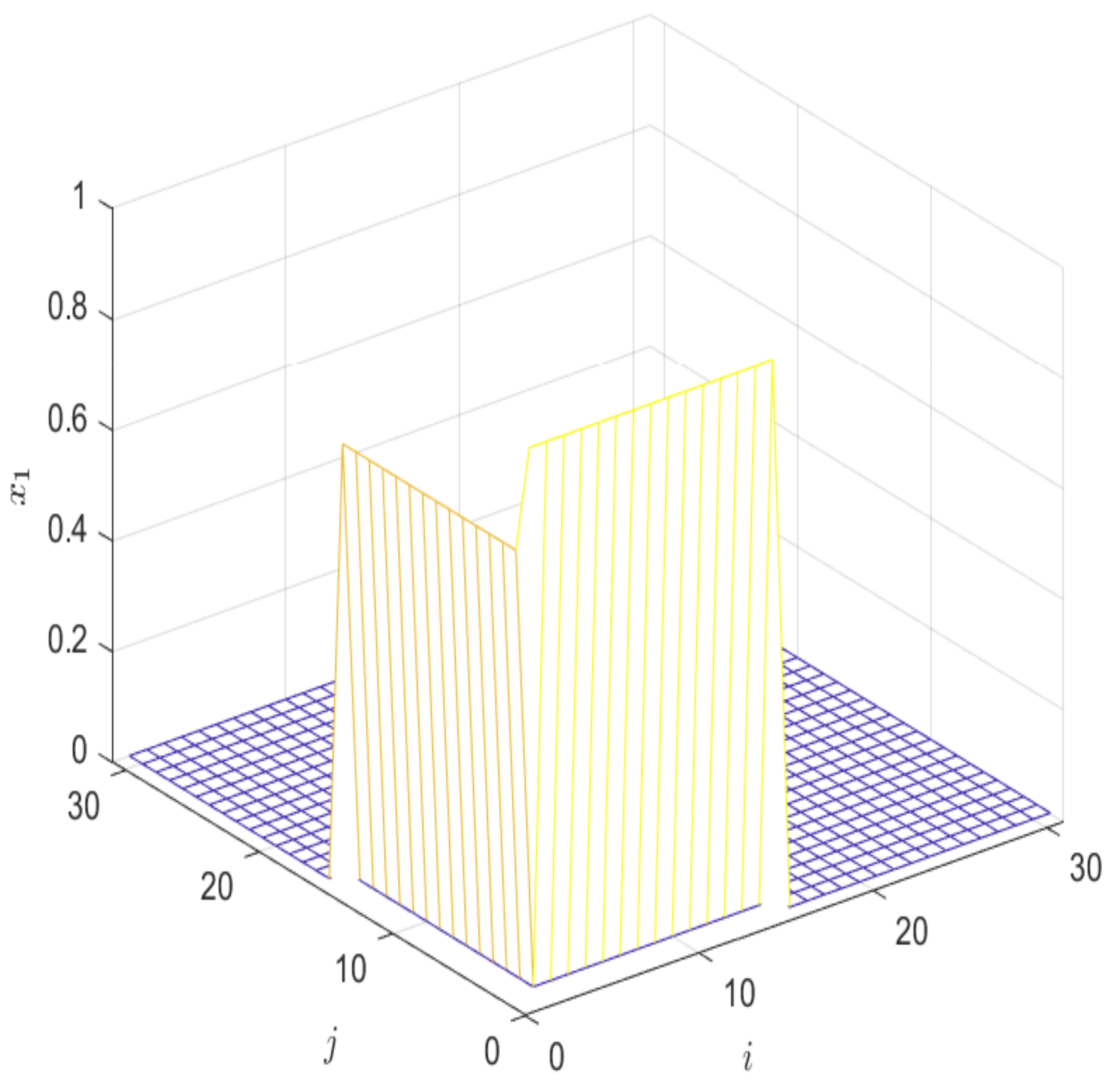
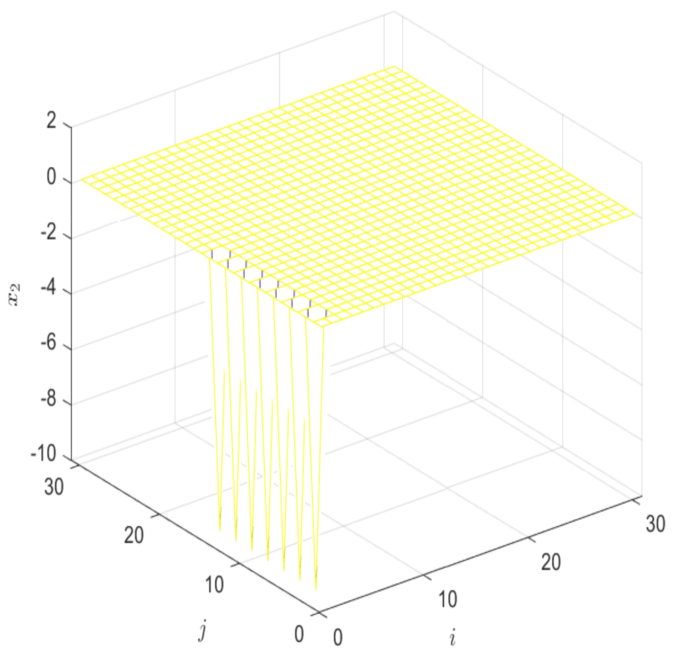
Suppose $\stackrel{-}{\beta }=0.55,\mu =2.5$, we have ${\tau }_{\alpha }>{{\tau }_{\alpha }}^{*}=1.9635$. Therefore, it can be seen that the closed-loop system can be stabilized under the restricted switching signal by the designed controller, and its average dwell time satisfying ${\tau }_{\alpha }>1.9635$. we choose ${\tau }_{\alpha }=2$, and the switching signal is shown in Figure 1, where 1, 2 and 3 represent the first, second and third subsystems, respectively. Giving the initial value $x_{i,0}$ and $x_{0,j}$, that satisfy the interval $[-1,1]$. Figure 2 and Figure 3 show the states of the open-loop system, it can be seen that the open-loop system is not stable. The states of the closed-loop system are shown in Figure 4 and Figure 5, it can be seen that the closed-loop system is stable.

6. Conclusions

This paper studies the stability analysis and controller design of a 2-D switched system based on the FMLSS model for arbitrary switching. The random disturbance is introduced into the discrete 2-D switched system model, and the sufficiency criterion of the mean square asymptotic stability of the discrete random 2-D switched system under any switching signal and the existence condition of the controller are obtained. In the 2-D switching system, the concept of instant is introduced, and the average residence time method is adopted under the restricted switching signal, and the stability conditions and the existence conditions of the controller under the restricted switching signal are given. Furthermore, express it as a linear matrix inequality condition. The result can be solved effectively by MATLAB software. Finally, an example is used to illustrate the validity of the theoretical analysis results.

References

1. Marszalek, W. Two-dimensional state-space discrete models for hyperbolic partial differential equations. Appl. Math. Model. 1984, 8, 11–14. [Google Scholar] [CrossRef]
2. Bouagada, D.; Dooren, P. On the stability of 2D state-space models. Numer. Linear Algebra Appl. 2013, 20, 198–207. [Google Scholar] [CrossRef]
3. Fornasini, E.; Marchesini, G. Stability analysis of 2-D systems. IEEE Trans. Circuits Syst. 1980, 27, 1210–1217. [Google Scholar] [CrossRef]
4. Paszke, W.; Lam, J.; Gałkowski, K.; Xu, S.; Lin, Z. Robust stability and stabilisation of 2D discrete state-delayed systems. Syst. Control Lett. 2004, 51, 277–291. [Google Scholar] [CrossRef]
5. Gao, H.; Lam, J.; Wang, C.; Xu, S. Robust H filtering for 2D stochastic systems. Circuits Syst. Signal Process. 2004, 23, 479–505. [Google Scholar] [CrossRef] [Green Version]
6. Zhao, D.; Ding, S.X.; Karimi, H.R.; Li, Y. Robust H Filtering for T wo-Dimensional Uncertain Linear Discrete Time-Varying Systems: A Krein Space-Based Method. IEEE Trans. Autom. Control 2019, 64, 5124–5131. [Google Scholar] [CrossRef]
7. Rongni, Y.; Yaru, Y. Event-triggered control of discrete-time 2-D switched Fornasini–Marchesini systems. Eur. J. Control 2019, 48, 42–52. [Google Scholar]
8. Ligang, W.; Rongni, Y.; Peng, S.; Xiaojie, S. Stability analysis and stabilization of 2-D switched systems under arbitrary and restricted switchings. Automatica 2015, 59, 206–215. [Google Scholar]
9. Xiang, W.; Xiao, J. Stabilization of switched continuous-time systems with all modes unstable via dwell time switching. Automatica 2014, 50, 940–945. [Google Scholar] [CrossRef]
10. Zhu, L.; Qiu, J.; Karimi, H. Region Stabilization of Switched Neural Networks With Multiple Modes and Multiple Equilibria: A Pole Assignment Method. IEEE Trans. Neural Netw. Learn. Syst. 2019, 31, 3280–3293. [Google Scholar] [CrossRef]
11. Wang, Y.E.; Sun, X.M.; Mazenc, F. Stability of switched nonlinear systems with delay and disturbance. Automatica 2016, 69, 78–86. [Google Scholar] [CrossRef] [Green Version]
12. Benzaouia, A.; Abdelaziz Hmamed, F.T.; Hajjaji, A.E. Stabilisation of discrete 2D time switching systems by state feedback control. Int. J. Syst. Sci. 2011, 42, 479–487. [Google Scholar] [CrossRef]
13. Xiang, Z.; Huang, S. Stability analysis and stabilization of discrete-time 2D switched systems. Circuits Syst. Signal Process. 2013, 32, 401–414. [Google Scholar] [CrossRef]
14. Shuang, S.; Zhongyang, F.; Weichao, S.; Yang, X. Stabilization of 2-D Switched Systems With All Modes Unstable via Switching Signal Regulation. IEEE Trans. Autom. Control 2018, 63, 857–863. [Google Scholar]
15. Fan, Y.; Wang, M.; Fu, H.; Zhang, B.; Bian, Y.; Sun, G. Quasi-Time-Dependent H Filtering of Discrete-Time 2-D Switched Systems with Mode-Dependent Persistent Dwell-Time. Circuits Syst. Signal Process. 2021, 40, 5886–5912. [Google Scholar] [CrossRef]
16. Gao, W.; Yang, Y.; Duan, H.; Li, M.; Ma, J.; Jin, S. Output Feedback Robust H Control for Discrete 2D Switched Systems. Comput. Syst. Sci. Eng. 2021, 39, 69–85. [Google Scholar] [CrossRef]
17. Ren, W.; Xiong, J. Robust Filtering for 2-D Discrete-Time Switched Systems. IEEE Trans. Autom. Control 2021, 66, 4747–4760. [Google Scholar] [CrossRef]
18. Badie, K.; Alfidi, M.; Chalh, Z. Exponential stability analysis for 2D discrete switched systems with state delays. Optim. Control Appl. Methods 2019, 40, 1088–1103. [Google Scholar] [CrossRef]
19. Kaiqun, Z.; Jun, H.; Yurong, L.; Naif, D.A.; Fuad, E.A. On l2l output-feedback control scheduled by stochastic communication protocol for two-dimensional switched systems. Int. J. Syst. Sci. 2021, 52, 2961–2976. [Google Scholar]
20. Branicky, M.S. Multiple Lyapunov Functions and Other Analysis Tools for Switched and Hybrid Systems. IEEE Trans. Autom. Control 1998, 43, 475–782. [Google Scholar] [CrossRef] [Green Version]
21. Liberzon, D.; Morse, A.S. Basic Problems in Stability and Design of Switched Systems. IEEE Control Syst. Mag. 1999, 19, 59–70. [Google Scholar]
22. Morse, A.S. Supervisory Control of Families of Linear Set-point Controllers-Part 11: Exact Matching. IEEE Trans. Autom. Control 1996, 41, 1413–1431. [Google Scholar] [CrossRef]
23. Ma, H.; Zhang, W.; Hou, T. Infinite horizon H2/H control for discrete-time time-varying Markov jump systems with multiplicative noise. Automatica 2012, 48, 1447–1454. [Google Scholar] [CrossRef]
24. Qi, Q.; Zhang, H. Output Feedback Control and Stabilization for Multiplicative Noise Systems With Intermittent Observations. IEEE Trans. Cybern. 2018, 48, 2128–2138. [Google Scholar] [CrossRef]
25. Ghous, I.; Xiang, Z.; Karimi, H.R. H control of 2-D continuous Markovian jump delayed systems with partially unknown transition probabilities. Inf. Sci. 2017, 382–383, 274–291. [Google Scholar] [CrossRef]
26. Jiang, B.; Karimi, H. Further criterion for stochastic stability analysis of semi-Markovian jump linear systems. Int. J. Robust Nonlinear Control 2020, 30, 2689–2700. [Google Scholar] [CrossRef]
27. Gao, H.; Lam, J.; Xu, S.; Wang, C. Stabilization and Stabilization of uncertain 2-D discrete systems with stochastic perturbation. Multidimens. Syst. Signal Process. 2014, 16, 85–106. [Google Scholar] [CrossRef]
28. Yao, J.; Ye, S.; Wang, W. Robust stabilization of 2D state-delayed systems with stochastic perturbation. In Proceedings of the 11th International Conference on Control Automation Robotics & Vision, Singapore, 7–10 December 2010; Volume 16, pp. 1951–1956. [Google Scholar]
29. Cui, J.; Hu, G. Stability for 2-D linear discrete systems with stochastic parameters. In Proceedings of the International Conference on Logistics Systems and Intelligent Management, Harbin, China, 9–10 January 2010; pp. 1243–1446. [Google Scholar]
30. Cui, J.; Hu, G. State estimation of 2-D stochastic systems represented by FM-II model. Acta Autom. Sin. 2011, 35, 755–761. [Google Scholar]
31. Yeganefar, N.; Yeganefar, N.; Ghamgui, M.; Moulay, E. Lyapunov theory for 2-D nonlinear Roesser models: Application to asymptotic and exponential stability. IEEE Trans. Autom. Control 2013, 58, 1299–1304. [Google Scholar] [CrossRef]
Figure 1. Switching signal.
Mathematics 10 00810 g001
Figure 2. State x 1 of the open-loop system.
Mathematics 10 00810 g002
Figure 3. State x 2 of the open-loop system.
Mathematics 10 00810 g003
Figure 4. State x 1 of the closed-loop system.
Mathematics 10 00810 g004
Figure 5. State x 2 of the closed-loop system.
Mathematics 10 00810 g005
Publisher’s Note: MDPI stays neutral with regard to jurisdictional claims in published maps and institutional affiliations.