2. Related Work
Recent studies [
9,
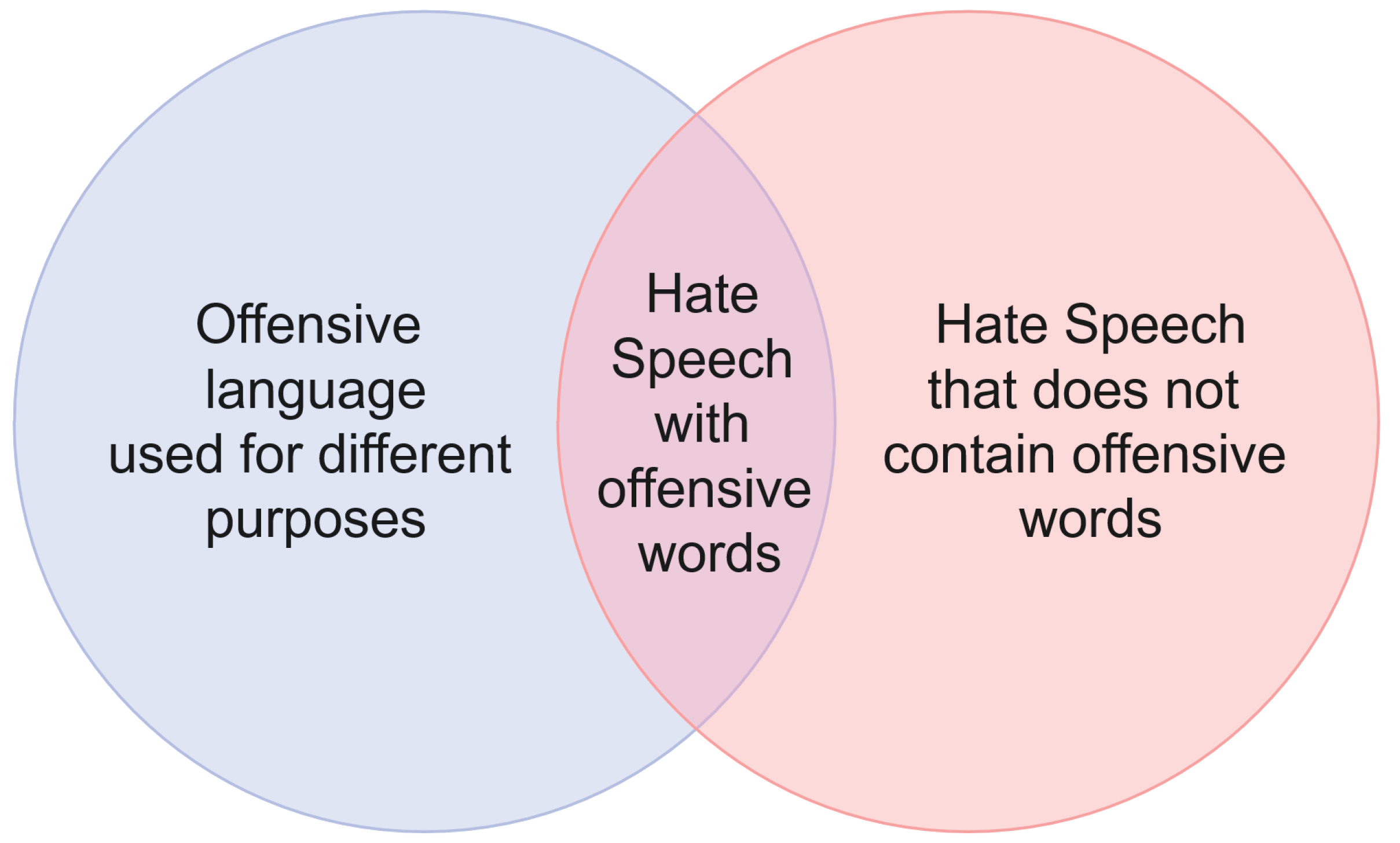
10] pertaining to the analysis of Hate Speech reveal that keywords are not enough in order to classify its usage. The semantic analysis of the text is required in order to isolate other usages that do not have the intention or meaning required for the phrase to be classified as Hate Speech. The outlined [
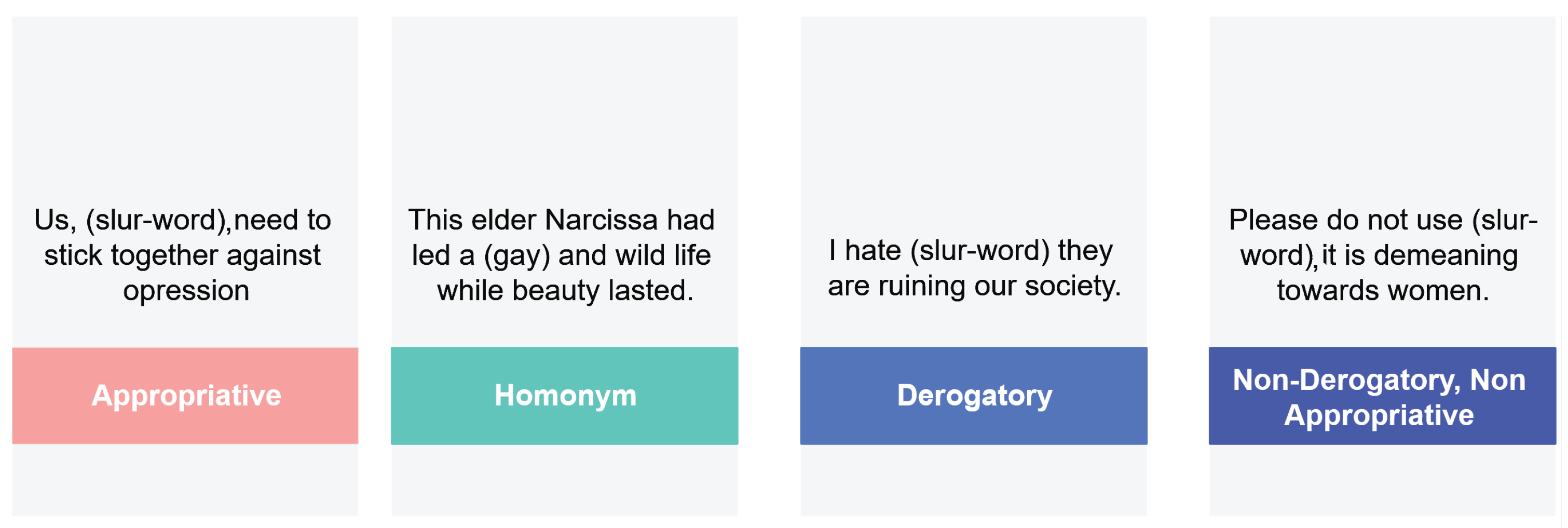
10] possible usages for Hate Speech words are:
Homonymous, in which the word has multiple meanings and in the current sentence is used with a different meaning that does not constitute Hate Speech;
Derogatory, this being the form that should be labeled as Hate Speech. This form is characterized by the expression of hate towards that community;
Non-derogatory, non-appropriative, when the keywords are used to draw attention to the word itself or another related purpose;
Appropriative, when it is used by a community member for an alternative purpose.
Figure 2 outlines examples of the presented ways of using Hate Speech key terms.
In recent years, a tremendous amount of research [
7,
8,
11] has gone into the classification of text snippets. Early methods relied on classic machine learning methods [
12] such as SVMs, logistic regression, naive Bayes, decision trees, and random forests. Even earlier research [
13] was focused on different ways of extracting textual features and text representations such as n-grams, lexicon, and character features. These laid a foundation for later research, which evolved with other related tasks, such as sentiment evaluation [
14], culminating with the usage of transformer-based neural networks [
15,
16].
The topic of Hate Speech detection is a very active part of the NLP field [
8,
15,
16,
17,
18]. Every modern advance in textual classification has been subsequently followed by an implementation in the field of Hate Speech detection [
15,
19,
20,
21].
One of the first modern articles was authored by Waseem and Hovey [
19] and consisted of Twitter detection work. Their paper used character n-grams as features, and they used the labels racism, sexism, and normal. The method used by the authors is a logistic regression classifier and 10-fold cross-validation in order to make sure the performance of the model is not dependent on the way the test and training data are selected. The preprocessing solution employed by the authors was removing the stop-words, special Twitter-related words (marking retweets), user names, and punctuation. This type of solution is commonly used in approaches where sequential features of the text are not used.
Another article, which constitutes the base of modern Hate Speech detection, is [
12]. The authors proposed [
12] a three-label Dataset that identifies the need to classify offensive tweets in addition to the Hate Speech ones of the Waseem and Hovey Dataset [
19]. Furthermore, the conclusion of the performed experiments was that Hate Speech can be very hard to distinguish from Offensive Language, and because there are far more examples of Offensive Language in the real world and the boundaries of Hate Speech and Offensive Speech intersect, almost 40% of the Hate Speech labeled tweets were misclassified by the best model proposed in [
12]. The article used classic machine learning methods such as logistic regression, naive Bayes, SVMs, etc. It employed a model for dimensionality reduction, and as preprocessing steps, it used TF-IDF on bigram, unigram, and trigram features. Furthermore, stemming was first performed on the words using the Porter stemmer, and the word-based features were POS tagged. Sentiment analysis tools were used for feature engineering, computing the overall sentiment score of the tweet. It is important to specify that only 26% of the tagged Hate Speech tweets were labeled unanimously by all annotators, denoting the subjectivity involved in labeling these kinds of tweets.
Modern approaches are highlighted by the use of embeddings and neural networks capable of processing sequences of tokens. One such article is [
17], in which the authors used ELMo embeddings for the detection of Hate Speech in tweets. Another technique that was present in this work was using one Dataset to improve performance on the primary Dataset (transfer learning).
The paper expressed this with a single-network architecture and separate task-specific MLP layers. In addition to these, the article compared the usage of LSTMs [
22] and GRUs [
23], noting that LSTMs are superior with respect to prediction accuracy. As preprocessing steps, the authors removed URLs and added one space between punctuation. This helps word embedding models such as GloVe, which would consider the combination of words and punctuation as a new word that it would not recognize. This article also introduced the concept of domain adaptation to Hate Speech detection. By using another Dataset to train the LSTM embeddings, the embeddings would be used to extract Hate-Speech-related features from the text, which would increase accuracy with subsequent Datasets.
One major downside of Hate Speech detection applications is given by the existing Datasets, which are very unbalanced (with respect to the number of Hate Speech labels), as well as by the small amount of samples that they contain. This means that the research in this field needs to make use of inventive methods in order to improve the accuracy. One such method is the joint modeling [
21] approach, which makes use of complex architectures and similar Datasets, such as the sentiment analysis ones, in order to improve the performance of the model on the classification of Hate Speech detection. In [
21], the use of LTSMs over other network architectures was also emphasized.
One of the more interesting models presented in [
21] is parameter-based sharing. This method distinguishes itself by using embeddings that are learned from secondary tasks and are combined with the primary task embeddings based on a learnable parameter. This allows the model to adjust how the secondary task contributes to the primary one, based on the relatedness of the tasks.
As preprocessing, the tweets had their mentions and URLs converted to special tokens; they were lower-cased, and hashtags were mapped to words. The mapping of hashtags to words is important because the tweets were small (the most common tweet size was 33 characters), so for understanding a Tweet’s meaning, we need to extract as much information from it as possible. Further improvement upon previous architectures within this model is the use of an additive attention layer.
As embeddings, GloVe and ELMo were used jointly, by concatenating the output of both models before passing it to the LSTM layer in order to make a task-specific embedding. This article [
21] also compared the difference between transfer and multi-task learning, with both having some performance boost over simple single-task learning.
Finally, there are multiple recent papers that made use of the transformer architecture in order to achieve higher accuracies [
8,
15,
16,
18]. One such transformer-based method [
8] that uses the Ethos [
24] Dataset employs a fairly straight forward approach. It uses BERT to construct its own word embeddings. By taking every corpus word and the context in which it occurs and constructing an embedding, the authors proposed that averaging word embeddings will have an advantage over other word embedding techniques. Then, by using a bidirectional LSTM layer, the embeddings were transformed into task-specific ones in order to improve accuracy, after which a dense layer made the prediction. The accuracy improved overall when this method was used as opposed to simple BERT classification. Another article that made use of the transformer architecture was [
15], introducing AngryBert. The model was composed of a multi-task learning architecture where BERT embeddings were used for learning on two Datasets at the same time, while LSTM layers were used to learn specific tasks by themselves. This is similar to the approach proposed in [
21], but the main encoder used a transformer-based network instead of a GloVe + ELMo embedding LSTM network. The joining of embeddings was performed with a learnable parameter as in [
21]. Another interesting trend is that of [
18], where a data-centric approach was used. By fine-tuning BERT [
25] on a secondary task that consisted of a 600,000-sentence-long Dataset, the model was able to generate a greater performance when trained on the primary Dataset.
Our approach complements those already used by proposing a method of encoding tokens that, while using the sub-word tokenizing architecture in order to handle new words, also makes use of the transformer performance, at the same time increasing the speed by running the transformer only to derive the embeddings. While RoBERTa-based transformer learning is still superior to using transformer-based token embeddings in terms of performance, if the training speed is of concern, then a viable alternative to the traditional multi-task learning methods and to the transformer-based paradigms is transformer-based token embeddings.
3. Materials and Methods
3.1. Datasets
This study wanted to determine if sentiment analysis Datasets, which by far outweigh Hate Speech ones in terms of data availability, can help in training for our Hate Speech detection problem. For this purpose, multi-task learning was used. Multi-task learning represents the method that leverages multiple learning tasks, trained at the same time, with the objective of exploiting the resemblances of the Datasets when training the parameters of the models. This method is used when the task is comprised of a very large Dataset for the secondary task and the primary (objective) task Dataset does not have sufficient data to produce an accurate result when trained by itself.
In order to conduct a comprehensive analysis of different methods used in Hate Speech detection and to study the effectiveness of each one of them, enough Datasets had to be gathered to test how these methods handle different sample types and labeling techniques.
Because there are different granularity levels for the labels, as well as the auxiliary data used by some models, in what follows, all the data collection processes that took place in the recreation of some of the more interesting state-of-the-art projects are explained. There are multiple types of Datasets already available, but the main concern of deciding which Datasets to use or how to construct a Dataset for the specific features of Hate Speech detection is choosing what features to leverage in this task and how those features can then be gathered in production environments. The main component of any Dataset should be the text itself, as this component allows us to examine the idea of the author of the sample at that particular time. Although it might be convoluted and new meanings of words appear all the time, the text feature is the easiest to retrieve from the perspective of a social platform owner as it is already in its database. This component is required for every employed Dataset and was constructed or harvested. If this was not possible, then the Dataset was discarded.
The Datasets chosen have different distributions of text length and different sources, which means that they were harvested from different social media platforms and use different labeling schemes. The most frequent labeling scheme observed is Amazon Mechanical Turk, but other crowdsourcing platforms [
12,
20,
26] are used as well. Finally, other authors manually annotated their Dataset or sought professional help from members of different marginalized communities and gender studies students [
10,
19].
By selecting different types of Datasets, the comprehensive testing of methods and the discovery of how different approaches to feature extraction and text embedding affect performance can be facilitated.
Labels of different samples can be binary or multi-class, as a result of evaluating them with multiple techniques, such as the intended meaning of the slur (sexist, racist, etc.) or what kind of slur word is being used (classifying each token as being Hate Speech or not). However, in order to standardize the labels, we split the Datasets into two Dataset groups (3-label and 2-label Datasets if they do not contain offensive speech labels). This was performed by merging or computing labels.
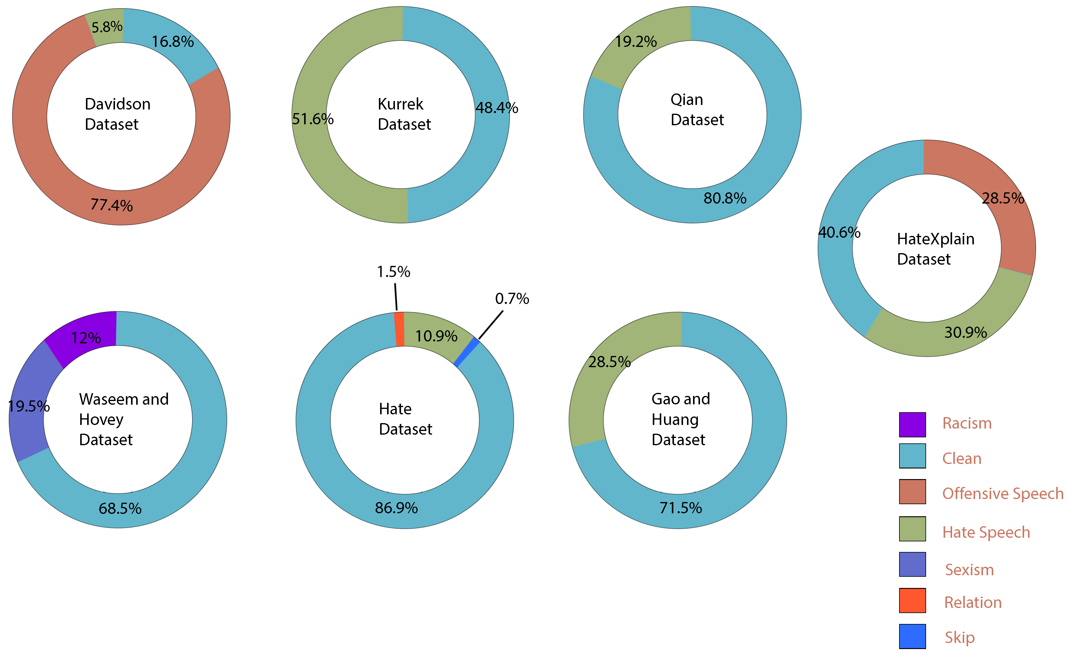
Secondary components that could help us determine if a person is posting Hate Speech content are: comments given by other people to that person’s post, user group names, user account creation timestamp (accounts participating in Hate Speech tend to be deleted so new accounts are created). Another secondary component that is recorded in some Datasets is user responses to the comment (not used for detection, but for generating responses to Hate Speech content). Some of these components were used, and the obtained accuracy was compared to the accuracy without them, in order to determine if there was an accuracy improvement over using text snippets only. Auxiliary Datasets, such as sentiment classification ones, can also be used (in multi-task learning). These Datasets do not have any constraints as they were only used to train the embedding vectors and, as such, to help the primary model’s accuracy. During our experiments, in addition to the Datasets presented in
Figure 3, the SemEval 18 [
27] Task1 Dataset (sentiment classification Dataset) and OLID (Hate Speech detection Dataset) were used as auxiliary Datasets in the sections where multi-task machine learning was performed.
A problem that was found while evaluating possible Datasets to be used for testing was that there are so many Datasets in the domain of Hate Speech detection, that the approaches presented alongside them have not been benchmarked on the same data.
3.1.1. The HateXplain Dataset
This Dataset [
11] contains already preprocessed tweets. It introduced the following token classes (<user>, <number>, <percent>, <censored>, etc.). In order to make sure this Dataset did not impact the pipeline, the tokens were implemented in the tokenizer so as to standardize every Dataset. Small problems were found with the human annotations: some of the annotators made mistakes such as when they considered more words than others for some sentences, for example the one at Index 17,891 (one annotator had 47 tokens, and another one had 48). The purpose of this Dataset was to use its attention annotations in order to harvest better scores in single-, multi-task, and transfer learning. Transfer learning is a method where the knowledge gathered while solving a secondary machine learning task is passed onto another similar task. One such example is attempting to predict sentiments that a text is supposed to convey and then taking that model and fine-tuning it in order to detect Hate-Speech-related texts. This technique is mostly used with the first layers of a deep neural network. The reason is that those layers are supposed to “understand” and to extract the features that are required by the later layers in order to make a decision.
3.1.2. The Waseem and Hovey Dataset
The raw data of this Dataset [
19] contains 16,914 tweets, annotated with the labels racist, sexist, and neither. The Dataset [
19] is available for download, but instead of Tweet text, its rows contain only tweet ids, and many of the tweets have been removed since its conception. However, some GitHub repositories might be used to combine the partial extraction attempts for obtaining over 90% of the original tweets. As for the original Dataset, the data are not balanced because the authors intended for it to represent a real-life scenario of Hate Speech detection. Furthermore, instead of basing their Hate Speech annotations solely on words that are commonly associated with Hate Speech, they labeled the tweets based on the significance of the tweet.
3.1.3. The Thomas Davidson Dataset
In [
12], the problem of differentiating between Hate Speech and Offensive Language that does not constitute Hate Speech was addressed. The Dataset is made up of tweets gathered using crowd-sourced Hate-Speech-related words and phrases from the website “
Hatebase.org”. The authors emphasized the difficulty of differentiating between tweets that contain offensive slurs that are not Hate Speech and Hate-Speech-containing tweets, as well as Hate Speech that does not contain offensive words. The authors constructed the labels by using CrowdFlower services. The agreement coefficient was 92%. During their examination of the Dataset, they found multiple mislabeled tweets. These had hateful slurs that were used in a harmless way, suggesting the bias towards misclassifying keyword-containing tweets. It is also important to remember that all labels were subjectively applied, and there is room for debate on the interpretation of some of the tweets being racist.
3.1.4. The Qian Reddit Dataset
This Dataset [
20] focuses on the intervention part of Hate Speech detection. The data were annotated using the Amazon Mechanical Turk crowdsourcing platform; this consists of Hate Speech annotations and responses to the Hate Speech samples. The authors focused on two platforms (Reddit and Gab) as the main sources of their Datasets. For the Reddit Dataset, the authors collected data from multiple subreddits known for using Hate Speech and combined this heuristic with hate keywords, then rebuilt the context of each comment. The context was made up of all the comments around the hateful comment. For the Gab Dataset, the same methods were applied. Conversations of more than 20 comments were filtered out. The authors obtained less accuracy on the Reddit Dataset, and that is why the models featured in this paper were trained only on this part of the data. After looking through the data, there were a couple of extra preprocessing steps that needed to be implemented when using this Dataset. For example, in the data, there were some Unicode characters such as “‘”, which is the Unicode variant of the apostrophe character. These need to be changed with their ASCII counterparts because of certain classic methods using the character as a separation of contractions.
3.1.5. The Kurrek Dataset
This Dataset [
10] is comprised of the Pushshift Reddit corpus, which is filtered for bots and users with no history. In addition to the user filters, which are designed to help future users collect user metadata and use them in combination with the Dataset, the corpus was selected to contain comments with 3 known Hate-Speech-related keywords. The Dataset is labeled in accordance with the use of the slur (derogatory usage, appropriative usage, non-derogatory, non-appropriative usage, and homonymous usage).
3.1.6. The Gao and Huang Dataset
The data records featured in [
28] were extracted from Fox news. The comments were taken from 10 discussion threads. The Dataset offers multiple metadata fields in addition to the sample text such as the nested nature of the comments and the original news article. The Dataset was annotated by two native English speakers.
3.1.7. Hate Speech Dataset from a White Supremacy Forum (the HATE Dataset)
The HATE Dataset, presented in [
29], is interesting because instead of searching a platform by keywords, which have a high probability of being associated with Hate Speech, the authors used web-scraping on a white supremacist forum (Stormfront) in order to improve random sampling chances. In addition to this, the Dataset has a skipped class where information not pertaining to being labeled can be classified. Furthermore, for some tweets, the context was used to annotate. We removed the classes skipped and those that needed additional context before training the models.
3.2. Types of Embeddings Used in this Paper
In order to display the evolution of different types of embeddings and to compare the difference in the training/prediction time with the difference in performance, this paper aimed to use the following embeddings for the tokens:
3.3. Evaluation
Hate Speech predictors focus on the macro F1 metric. This metric is especially important because the benign samples far outweigh the offensive ones. F1 is calculated as the harmonic mean of the recall and precision metrics. Furthermore, all metrics shown in this paper are macro, which means that the metrics are representative of all classes. The sampling procedure most used to evaluate classification models on a segmented Dataset is K-fold cross-validation. In the case of our tests, we chose 10-fold because it is the most popular for Hate Speech classification [
8,
19,
21].
3.4. Preprocessing
In order to make use of all the Dataset features, we needed to preprocess it according to all the tokenizing module requirements, so as to form the word vectors and embeddings, as well as to perform the existing preprocessing steps that some of the Datasets in use already employ.
The first step is adhering to GloVe’s special token creation rules. By following the token definitions in the paper, a script was created in order to create the tokens that were needed by GloVe. We used regex in order to create the tokens. The next preprocessing step was mandated by the HateXplain Dataset. The Dataset is already in a processed state. By searching for the pattern <Word>, a tokenizing program can be reverse engineered, at the end of which the embeddings are reconstructed (over 20 in the Dataset). Some of the words are censored, so in order to improve the accuracy of BERT, a translation dictionary can be created to accomplish this feat.
The final step was constructing two preprocessing pipelines, one for the HateXplain Dataset, in order to bring it to a standard format, and another preprocessing function was created for the other texts. Further modifications were needed for the other Datasets depending on how they were stored.
Because the study dealt with two different types of texts, the preprocessing should be different for each article. For the tweet Datasets/short-text Datasets, it is recommended that as much information as possible be kept, as these are normally very short. As such, the hashtags should be converted into text and emojis and other text emojis as well. For the longer texts, however, cleaner information had priority over harvesting the entire information, one such method difference being the deletion of emoticons instead of replacing them as in the tweet Datasets.
As such, the proposed pipeline for these kinds of models was, after preprocessing, composed of the following word embedding extraction methods:
N-gram char level features;
N-gram word features;
POS of the word;
TF (raw, log, and inverse frequencies)-IDF(no importance weight, inverse document frequency, redundancy);
No lemmatization running words were directly taken as input—no lemmatization, but unlemmatizable words were deleted;
GloVe
ELMo;
Transformers.
With the first types of models, multiple types of preprocessing were tested, in order to see which ones performed better than the others. One such example is represented by stemming and lemmatization. We tried different preprocessing steps in this first part of the Dataset, such as stemming or lemmatizing the words. Another preprocessing method that we tried was removing stop-words or using exclusively stop-words. We acknowledge that using our own encoding vector, as well as extracting word- or char-level features such as n-grams cannot be replicated on real-life data as easily as using already computed word embeddings such as GloVe or ELMo [
33,
35]. As such, we tried to only use open-source embedding methods on the classical machine learning algorithms.
All the classical machine learning models are formed of a sci-kit learn [
30] pipeline with different parameters (depending on the model used). In order to tune the parameters, we used grid search and studied the different effects that different parameters had on the accuracy of the models. Furthermore, for the PyTorch [
36] models, we additionally used ray tune from the PyTorch framework.
3.5. Optimizers
An optimizer is an algorithm that helps the neural network converge, by modifying its parameters, such as the weights and learning rate, or by employing a different learning rate for every network weight.
SGD [
37] with momentum is one of the simpler optimizer algorithms. It uses a general learning rate as opposed to the Adam optimizer [
38]. It follows the step size to minimize the function. Momentum is used to accelerate the gradient update and to escape local minima.
Adam [
38] is a good choice over stochastic gradient descent because it has a learning rate for every parameter and not a global learning rate as classical gradient descent algorithms. The original Adam paper [
38] claimed to combine the advantages of AdaGrad and RMSProp. The article claimed that the advantages of Adam were the rescaling invariance of the magnitudes of parameter updates to the rescaling of the gradient, the hyperparameter step size bounding the parameter step sizes, etc. The upper hand Adam has as an optimizer is generated by its step size choice update rule.
RMSProp is different from Adam as it does not have a bias correction term and can lead to divergence, as proven in [
38]. Another difference is the way RMSProp uses momentum to generate the parameter updates.
AdaGrad [
39] is suitable for sparse data because it adapts the learning rate to the frequency with which features occur in the data. It was used in [
32] because of the sparsity of some words. AdaGrad is similar to Adam because it has a learning rate for every parameter. The main fault is adding the square gradients, which are positive. For big sets of data, this is detrimental as the learning rate becomes very small.
3.6. Models
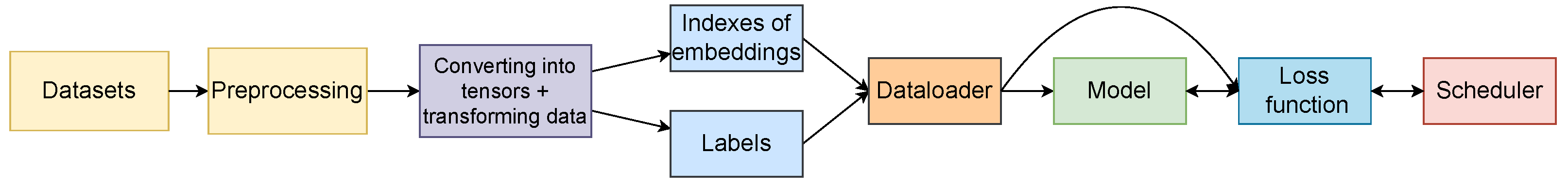
In order to test the methods, we propose the pipeline in
Figure 4.
In order to streamline the process, the Datasets can be saved after preprocessing and then loaded up so as to not repeat this part of the experiment on subsequent tests. In addition to this, the model weights can be reset, as opposed to training the model again for the next folds, while performing the validation.
3.6.1. Classic Machine Learning
Our initial tests concentrated on classical machine learning models, and their results can be seen in
Appendix A. The first models that were applied were from the family of SVM classifiers (
Table A2). These classifiers work by establishing the biggest boundary between classes. The kernel function that differentiates between SVM methods helps shape the boundary and, as such, the decision-making capabilities of SVM classifiers. All the classic machine learning models are formed of a sci-kit learn pipeline with different parameters (depending on the model used).
In order to tune the parameters, we used grid search and studied the different effects that various parameters had on the accuracy of the models.
Other classifiers that were used during the first phase of the model preparation were decision tree classifiers (
Table A3), which construct a tree-like structure. The goal was that of differentiating between classes based on boundaries set automatically by the algorithm. Furthermore, random forest (
Table A4) and KNN classifiers (
Table A1) were tested. Random forest classifiers work by combining multiple different decision tree classifiers, and KNN classifiers compare the similarity of the nearest neighbors and decide based on the labels of those neighbors.
The obtained results enabled us to conclude that, on this tier of classic machine learning classifiers, the SVM and random forest classifiers outperformed the rest of the models on the task of Hate Speech detection. The features were derived from the text using TF-IDF.
3.6.2. CNN, GRU, and RNN Models
The next class of tested models was represented by CNN-based models. These had better accuracy than obtained for the previous phase. As input for the network, GENSIM embeddings (either Cbow or skip-gram of dimension 200) trained on the Datasets were used. These were compared against GloVe embeddings in order to test which embeddings would be more appropriate for the task of Hate Speech detection. GloVe embeddings scored a higher accuracy overall, and because of this, they were used for the more advanced models.
There were multiple CNN approaches tested for this study. The first type has a bigger number of filters, essentially capturing more patterns from the texts, but fewer layers. Other CNN networks have a shorter filter size, but more layers so as to further refine the representations gathered from the text (
Table A6). These approaches were used in order to establish if extracting more features from the text was more important than filtering and extracting more complex patterns.
Another tested model was described in [
11] and is made up of convolutional neural networks combined with a GRU layer (
Table A9). This model outperformed the other two. During the testing of this model, we also tested how skip-gram embeddings affect performance versus a more established embedding method.
Furthermore, several RNN setups have been tested, both bidirectional RNN (
Table A7) and one-way interconnected RNN (
Table A8) networks.
3.6.3. Preparing the Data for Recurrent Layers
In order to use recurrent networks, some precautions must be taken. For the LSTM, GRU, and RNN networks, the main methods for input encapsulation are as follows:
Padding sequences of data to a fixed length represents the easiest way of preparing the input for recurrent layers. For this method to work, we needed to choose the correct length of the sentence. The length must be large enough so that we have a low probability of losing the meaning of the sequence (by not cutting out words that would be crucial to the understanding of the sentence). At the same time, this length must be small enough such that, when the input is grouped together, the batch fits on the GPU/TPU and the training/prediction time is reasonable.
In addition to the token length, one must consider the batch size. It is important to make sure that the GPU can handle the size of the model training/prediction data flow.
When testing on the tweet-based Datasets, the method chosen was to keep all input words and pad the shorter input samples to the same length. For tweet samples, this is easy as there is a limit to how many words a tweet can contain. As for our Datasets, the limit ranged from 70 to 90 tokens. Some words can be split by the sub-word tokenizer into two or more tokens, so based on what method of tokenization is chosen, the limit was either 70 or 90 tokens. However, handling inputs from Gab or Reddit, with sizes of over 330 words, required a different approach. For such Datasets, the Dataset length chart is plotted, and we considered the length that separates the smallest 95% of the samples, from the rest, as a cutoff point. The longer texts were then cut to that length, and all the shorter texts were padded to the same length;
The second approach was packing the variable length sentences and unpacking them after the LSTM layer has finished. This approach is supported by PyTorch. It works by capturing LSTM inputs at the sequence when the true input ends.
These models performed poorly in comparison with the LSTM and transformer networks.
3.6.4. LSTM Based Networks
One of the more complex classification criteria for the models used in the experiments was whether they trained on one task or multiple tasks at the same time, with the goal of perfecting the training on one of them, called the primary task.
The single-task learning model was trained only on one Dataset. It can have one or multiple vector embedding inputs (GloVe (
Table A5), GloVe + ELMo (
Table A13), ELMo, BERT, BERT + GloVe, etc.). Parameters such as LSTM hidden sizes and dropouts were computed based on grid search on one Dataset and then reused in the testing on subsequent Datasets.
After the LSTM layers process the input, the output has to be reshaped and pooled in order to be used in future layers. If the input goes into other LSTM or time sequence computing layers, we kept the output as is, but if we intended to forward the output to the multilayer perceptron, we only took the last sequence embeddings. In order to achieve this, the matrix returned by the LSTM layer needed to be reshaped according to the following parameters: the number of layers, the number of directions, the batch size, and the hidden dimension of the LSTM layers. The last element of the output vector was used, and if the LSTM was bidirectional, both LSTM outputs needed to be concatenated. After each LSTM layer, there was a dropout layer that helped with overfitting.
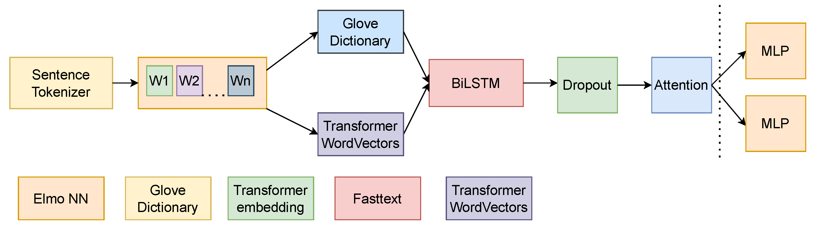
The linear layer was composed of multilayer perceptrons, and its purpose was to reduce the pooled output of the BiLSTM to our label size. The last layer can be reset if we want to train multiple Datasets on the same model. The goal of this procedure is improving the accuracy of the model on the last Dataset (as in
Figure 5).
3.6.5. Improving the LSTM Output
Other changes between models included, but were not limited to, the addition of an attention layer instead of the max pooling layer of the first model architecture.
The attention layer had the basic function to produce weights that helped a model focus on certain words in the sentence such that its accuracy was increased. Despite attention being used primarily in seq-to-seq translations, in order to relieve the encoder from condensing the data into a fixed-length sequence, it is also useful in classification scenarios, when we want to take advantage of the sequential nature of LSTMs. In our classification scenario, for each embedding dimension of a LSTM step, we had a weight that decided its importance. The weight was at the end multiplied with all the encoding vectors. We can replace the traditional max pooling approach or just use the output of the last layer and input it into the already described attention mechanism. The attention layer helps the model properly focus on the parts of the samples that help produce the right label.
3.6.6. Multi-Task Learning Models
Multi-task models require a different approach for training. First, the labels must be encoded such that there can be a distinction between our primary and alternate Datasets. In order to do this, a label value that was not in our Dataset was inserted (for example, 2 in binary classification, where there would be only 0 and 1 labels).
Every sample from the auxiliary Dataset was marked with the chosen label in the primary label column. Then, the secondary Dataset labels were placed in another column. For testing purposes, the fields that correspond to the unused label were filled with a random label that did not exist in our Datasets, such that, if there was an error and the separation of labels was not properly preformed, that error could propagate into the confusion matrix and be corrected. During training, both samples were dispatched to the embedding stage of samples and were then filtered in the order of the labels. The losses were computed separately and were afterwards multiplied by a factor (0.9 for our primary Dataset and 0.1 for our secondary Dataset). In the end, the weights were updated with backpropagation, and the model was trained. There were 3 types of multi-task learning models that were studied for the task under investigation. They were tested according to their description in [
21].
The first tested multi-task model was “hard” multi-task learning (
Table A11). This model has 3 separate BiLSTM structures. The first is composed of 2 layers and is used to process inputs from both the auxiliary and primary tasks. The second and third structures are task-specific, used to further enhance the representations given by the output of the first BiLSTM structure. There are two different loss calculation paths that intersect at the first BiLSTM structure. This means that, although task-specific representations would be trained separately, the first structure was jointly learned. This helped our primary task if sufficient data were not available, as well as in cases where these tasks were similar in nature.
Another variant, that is easier to train, was also designed and tested. This model does not contain the separate BiLSTM layers, but instead contains only one representation that is then separated into different dense layers (
Table A12). The rationale was that the LSTM layers will interpret the sentences, and the output of the last layer will treat both tasks, which is why the BiLSTM-tested hidden dimensions would be larger than in previous models.
3.6.7. Learnable Parameter Multi-Task Learning Models
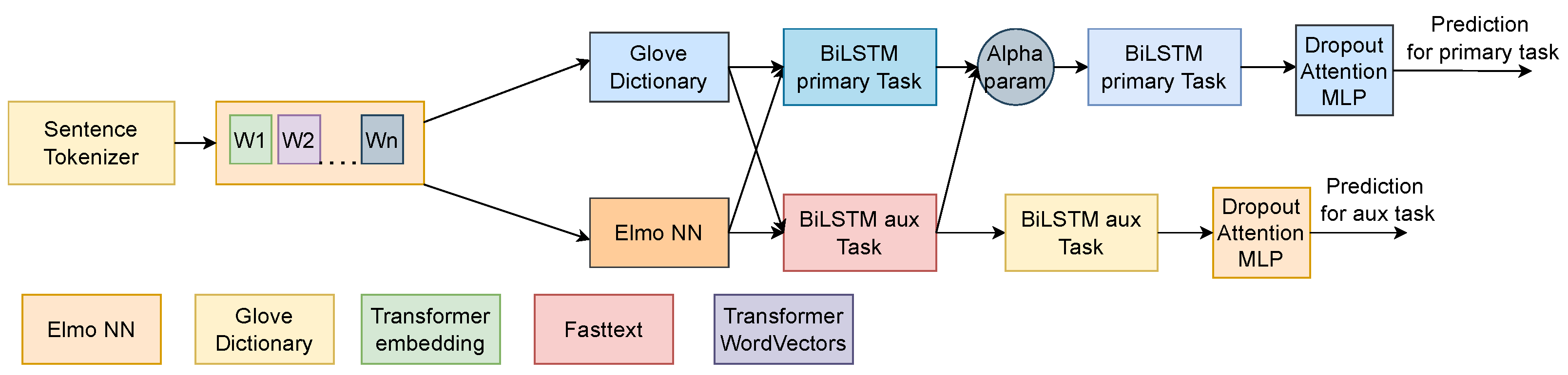
Another multi-task learning model is obtained by having a learnable parameter (
Table A10,
Figure 6), as depicted in [
21]. For the implementation in PyTorch, a random tensor was made (containing 2 values, initialized with Xavier initialization), after which gradients were enabled on that tensor so that the backpropagation could change its value.
When the BiLSTM results were to be concatenated, SoftMax was applied on the parameter tensor, which normalizes the 2 values in the vector as a probability distribution (they are complementary, summing to 1). Then, each corresponding embedding is multiplied with its corresponding vector value. Other modifications were that the common BiLSTM layer no longer existed, so that each task built its own interpretation of the input sequence. As a sanity check, as the one in the previous example, a model was built that was trained in the same manner, but without connecting the BiLSTM of the auxiliary model to the Alpha parameter. If both models performed identically, this meant that there was no performance gain out of using a flexible parameter multi-task model.
3.6.8. Speed, Ease of Training, Sanity Checking, and Other Particularities
The GloVe model was the easiest to train, with 10 min per epoch on the largest Dataset (combined two-label Dataset). On the other side, there was the multi-task parameter model, which took 2 h and 30 min per epoch (both models were trained on a server V100 graphics card with 16 GB or VRAM). Because the majority of the multi-task models were bigger than the 12 GB of video RAM of the NVIDIA 3060, it is harder for a consumer GPU to train them, as the batch sizes have to be set low in order to not overflow the GPU memory. Furthermore, a compromise between performance and ease of training has to be made, and that could be using token embeddings derived from transformer models combined with the speed of single-task models.
In order to test if the design of multi-task architectures improved the performance of the model, a testing architecture was conceived by us. It follows the same paths as in the case of the above-presented hard multi-task models, except that it is missing the first BiLSTM structure (which learns the shared embedding). This impairs shared learning, but the process of training is exactly the same. When testing this model, if observing the same performance, we could conclude that there was no performance gain in hard multi-task learning.
As optimizers, two types were tested: Adam and SGD with momentum. In practice, Adam seemed to be a better fit for this task, especially the corrected method AdamW implemented in PyTorch. As loss functions, binary cross-entropy loss was used for the models, which requires binary classification, and categorical cross-entropy loss was used for models that require multiple class classification.
3.6.9. Transformer-Based Models
Our study used the BERT model in 3 architectural ways.
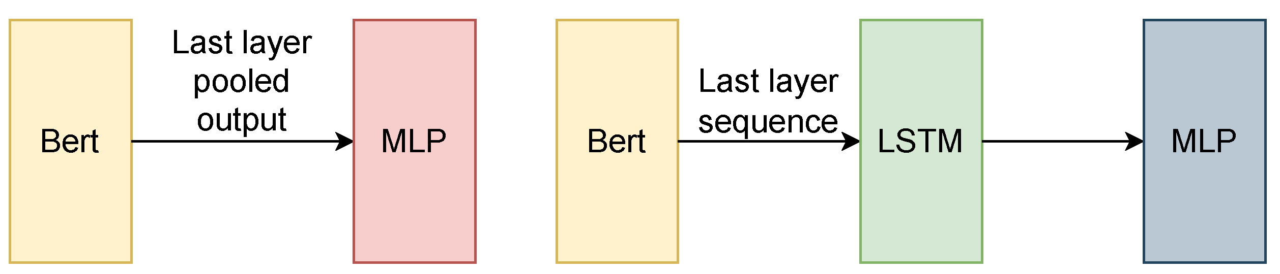
The first and most basic way in which we could employ BERT (presented in
Figure 7) was by using the BertForSequenceClassification function in PyTorch. The model should be trained according to the original paper [
25] that introduced it:
Batch size should be 16 or 32;
Learning rate for Adam optimizer should be 5 × 10, 3 × 10, or 2 × 10;
Number of epochs should be small. between 1 and 5.
The second possibility is using Bert’s output layer as an input to a multilayer perceptron or any other non-sequential network. The training was performed by freezing the BERT layers and training the rest of the network, then unfreezing the BERT layers and adjusting the optimizer, learning rate, and batch size to the ones in the above guidelines, as well as retraining for a small number of epochs [
11].
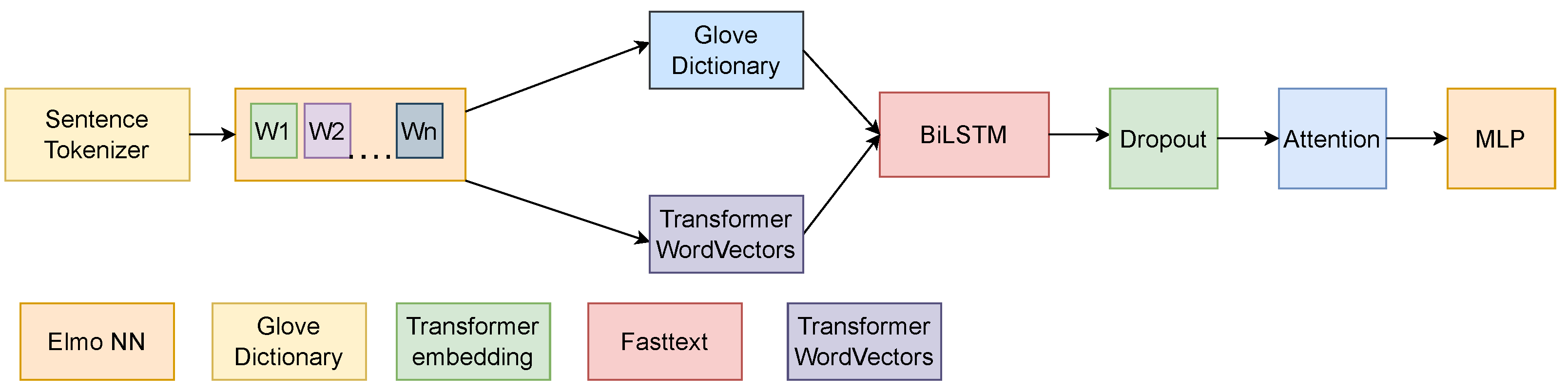
The final method in which BERT can be used is for embedding vector creation. By freezing the weights as in the previous model, we could use the sequential output of BERT as a word embedding vector. In some of the experiments, the coupling of transformer-based models together with GloVe embeddings was tested in multiple multi-task learning use cases, as well as in single-task use cases, as depicted in
Figure 8. BERT was used in combination with GloVe in two ways: by using it as an embedding vector or as a sequential model. The training was identical to the above-described process.
While training the transformer-based models, one problem was the high cost of training, as well as the longer training time than for LSTM-based networks, and as such, a good method was stated by [
8]. Instead of taking the word-level embeddings as in [
8], we used the RoBERTa tokenizer to obtain token-level embeddings for multiple Datasets. Using those embeddings, we then trained a multi-task architecture based on bidirectional LSTM networks with an addition-based attention mechanism.
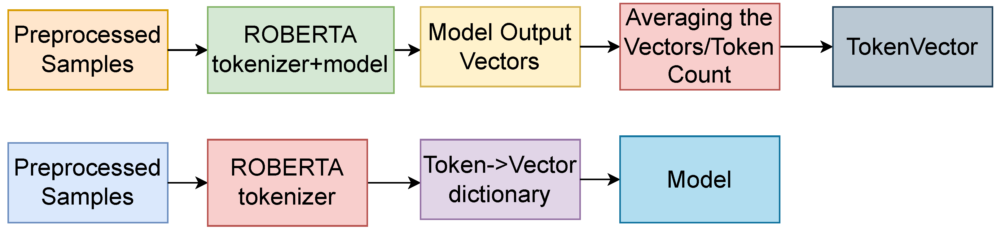
The pipeline began with the sentence, which was tokenized using the standard BERT/RoBERTa tokenizer (depending on the model used). Then, each sample was input into the model (standard model with no gradients computed to save the GPU), and after obtaining the embeddings from the models, we assigned them to each of the tokens that served as the input. We summed up all the different representations a token would have, within the Dataset, and in the end, we averaged the vectors for each token, by dividing the token vector by the number of times the token had occurred throughout the Dataset. In the end, we converted the embeddings to PyTorch embeddings, because it was much faster than using a Python dictionary.
For the next batch of models, we employed the multi-task architecture with word embeddings computed using the RoBERTa-based model. For this purpose, we took all the Datasets, as well as the auxiliary Datasets, and we created token vectors for all of them. The process of obtaining transformer token vectors is depicted in
Figure 9.
3.6.10. BERT Token Embeddings for Single-Task Learning
The first experiments involving transformer-based token embeddings consisted of using the BERT-based token embeddings with an additional LSTM layer. By doing this, we obtained the approximate performance of the BERT model alone, but with a speed advantage given by using word embeddings.
3.6.11. RoBERTa Token Embeddings for Multi-Task Learning
Secondary experiments were composed of using multi-task experiments by combining the SemEval Dataset with all the different Datasets. As word embeddings, the RoBERTa-derived token embeddings were used. While testing, transformer-based architectures proved far superior to the GloVe and ELMo embeddings, and among the transformer models, RoBERTa had the highest accuracy on the Hate Speech Datasets. The three multi-task architectures outlined in [
21] were adapted to use RoBERTa word embeddings instead of the standard ones.
3.6.12. Training Particularities
During the training, all the models converged. However, employing early stopping mechanisms and tuning the hyperparameters helped the models achieve better results. A problem was using larger text Datasets with multi-task learning. It would not be suitable for texts over 250 words, as the batch size would have to be considerably reduced, in order to facilitate the training. Another problem is not using the same type of text for the primary and auxiliary Datasets. If this constraint is not met, then the primary Dataset will have a hard time surpassing the single-task learning method accuracies.
5. Conclusions and Future Work
With “Hate Speech” being the next term to be criminalized at the EU level and with growing activity on social media, automatic Hate Speech detection increasingly becomes a hot topic in the field of NLP. Despite a relatively large and recent amount of work surrounding this topic, we note the absence of a benchmarking system that could evaluate how different approaches compare against one another. In this context, the present paper intended to take a step forward towards the standardization of testing for Hate Speech detection. More precisely, our study intended to determine if sentiment analysis Datasets, which by far outweigh Hate Speech ones in terms of data availability, can help train a Hate Speech detection problem for which multi-task learning is used. Our aim was ultimately that of establishing a Dataset list with different features, available for testing and comparisons, since a standardization of the test Datasets used in Hate Speech detection is still lacking, making it difficult to compare the existing models. The secondary objective of the paper was to propose an intelligent baseline as part of this standardization, by testing multi-task learning, and to determine how it compares with single-task learning with modern transformer-based models in the case of the Hate Speech detection problem.
The results of all the performed experiments point to the fact that using transformer models yielded better accuracies overall than trying token embeddings. When speed is a concern, then using token embeddings is the preferred approach, as training them used less resources and yielded a comparable accuracy. Using auxiliary Datasets helped the models achieve higher accuracies only if the Datasets had the same range of classification (sentiment analysis or Offensive Language detection were complementary for Hate Speech), but also the same textual features (using tweet Datasets for longer text Datasets can be detrimental to its convergence).
Although the detection of Hate Speech has evolved over the last few years, with text classification evolving as well, there still are multiple improvement opportunities. A great advancement would be to train a transformer on a very large Hate Speech Dataset and then test the improvement on specific tasks. In addition to these, various other Dataset-related topics should be addressed, such as the connection between users or different hashtags and movement names and how these factor into detecting Hate Speech. That issue could be addressed by a combination between traditional approaches and graph neural networks. Furthermore, it would be interesting to receive a Dataset with all the indicators a social media platform has to offer.
One downside of current Datasets is the fact that, during our experiments, as well as during other experiments in similar works, non-derogatory, non-appropriative, as well as appropriative uses of Hate Speech words were very hard to classify, as they represent a very small portion of the annotated tweets. These kinds of usages should not be censored as they are impacting the targeted groups. Another example of Hate-Speech-related word usage, that is hard to classify, would be quoting a Hate Speech fragment of text with the intent to criticize it. Improvements in neural networks would have to be made in order to treat these kinds of usages.
As future work, we plan on expanding our testing on Datasets that subcategorize the detection of Hate Speech into different, fine-grained labels. One such Dataset that was used in this paper is the Waseem and Hovey Dataset [
19]; another one should be SemEval-2019 Task 5 HatEval [
40], which categorizes Hate Speech based on the target demographic. It would be interesting to observe how well features learned during a more general classification could be used to increase the classification accuracy of a finer-grained task. Moreover, another direction that this research could take is to expand the types of NLP applications for which the methods are tested. One such example would be handling Hate-Speech-related problems such as misogyny identification [
41]. We hope the present study will stimulate and facilitate future research concerning this up-to-date topic, in all of these directions and in others, as well.


