
A Modified Power Family of Distributions: Properties, Simulations and Applications


Abstract
:1. Introduction
2. Materials and Methods
2.1. The New Family
- (i)
- If is monotone increasing and then for all x.
- (ii)
- If is monotone decreasing, and then for all x.
- (iii)
- if .
- (iv)
- if .
2.2. Moments
2.3. Generating Function
2.4. Quantiles
2.5. Mode
2.6. Hazard Rate
2.7. Estimation
3. Sub-Models
3.1. Modified Power Exponential (MPoE)
3.2. Modified Power Weibull (MPoW)
3.3. Modified Power Fréchet (MPoF)
4. Applications
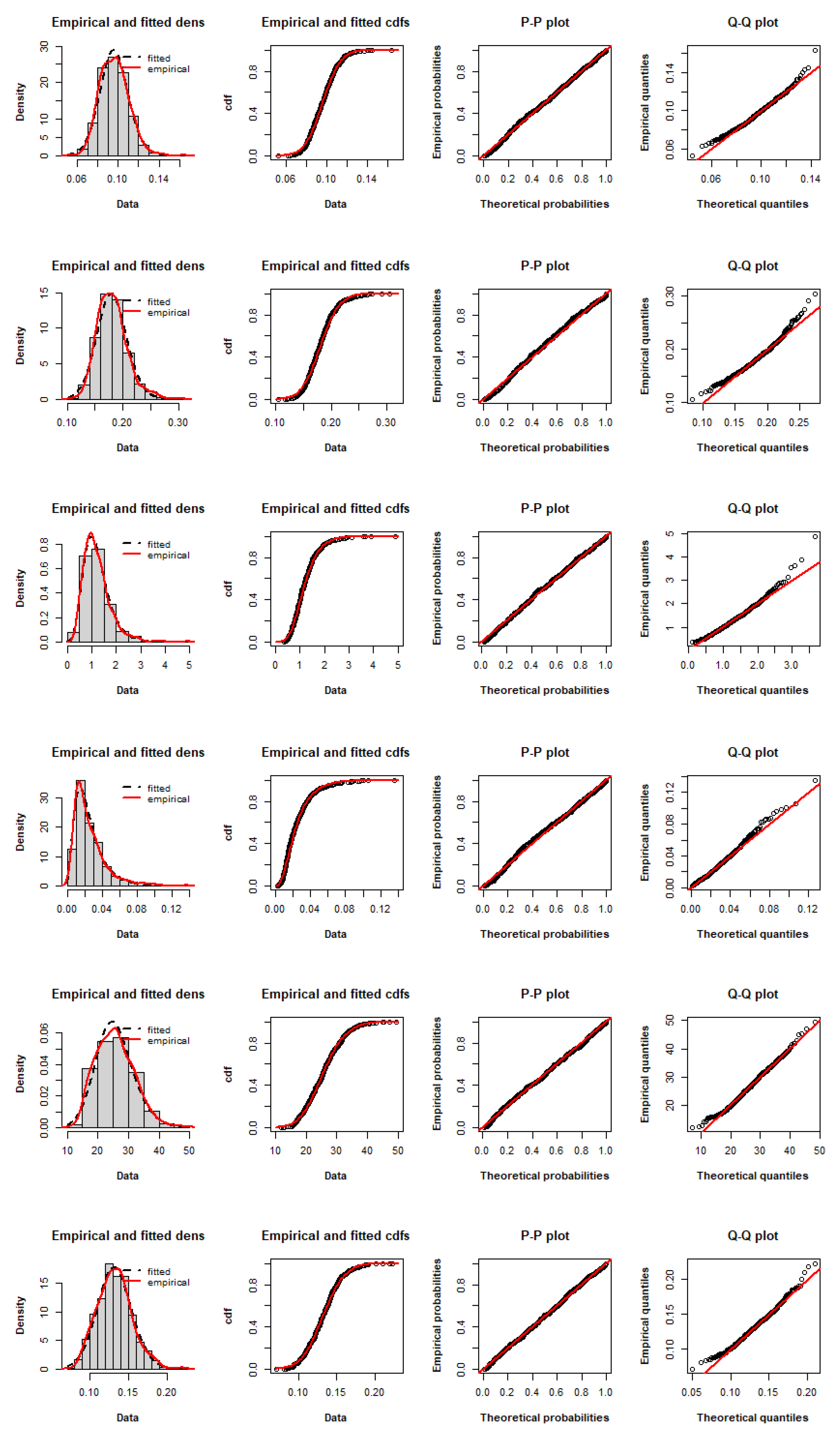
4.1. Simulation Results
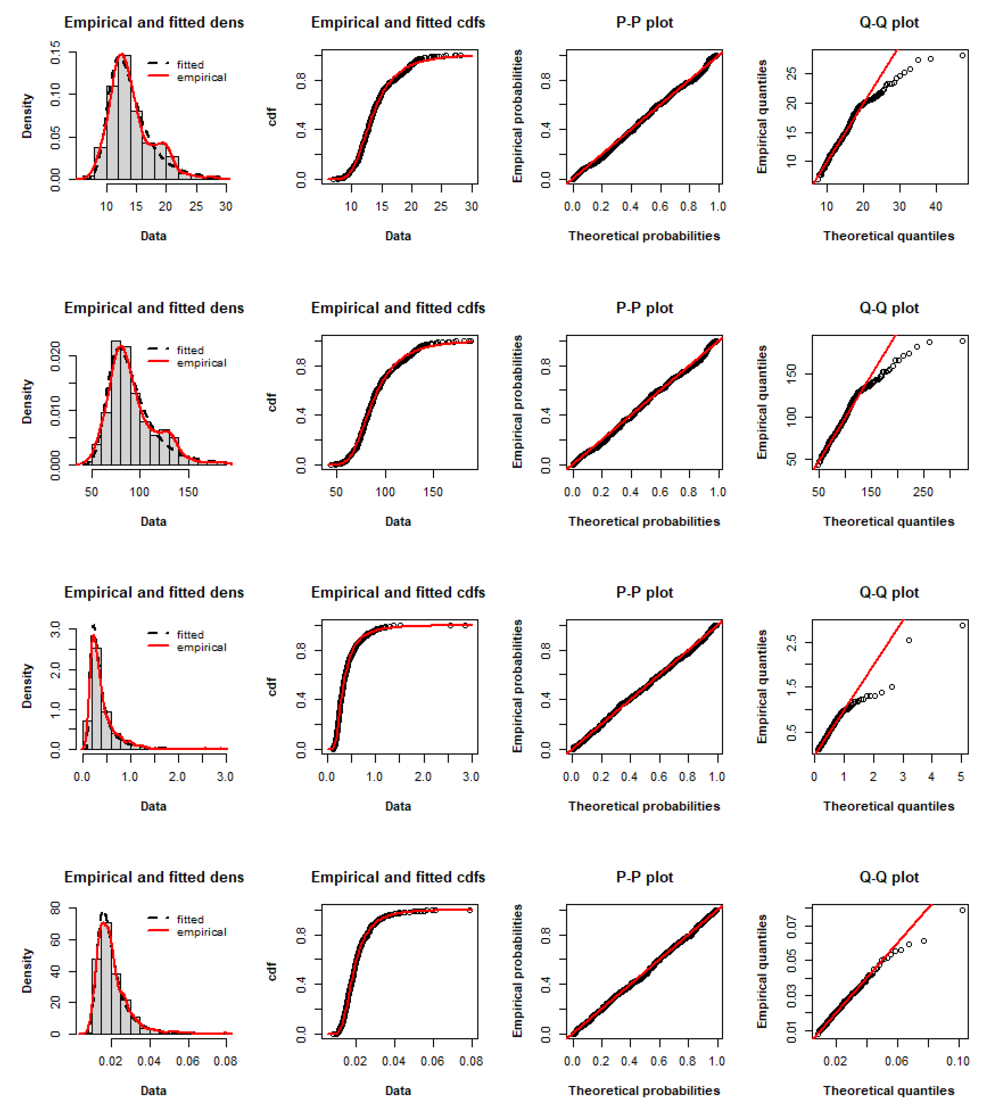
4.2. Real Data
4.2.1. Breast Cancer Data
4.2.2. Coal-Mining Data
5. Conclusions
Author Contributions
Funding
Institutional Review Board Statement
Informed Consent Statement
Data Availability Statement
Conflicts of Interest
Abbreviations
| AB | absolute bias |
| cdf | cumulative distribution function |
| CI | confidence interval |
| CvM | Cramér–von Mises |
| hrf | hazard rate function |
| KS | Kolmogorov–Smirnov |
| MLE | maximum likelihood estimate |
| P-P | probability vs. probability |
| probability distribution function | |
| Q-Q | quantile vs. quantile |
References
- Marshall, A.W.; Olkin, I. A New Method for Adding a Parameter to a Family of Distributions with Application to the Exponential and Weibull Families. Biometrika 1997, 84, 641–652. [Google Scholar] [CrossRef]
- Ghitany, M.E.; Al-Hussaini, E.K.; Al-Jarallah, R.A. Marshall-Olkin Extended Weibull Distribution and Its Application to Censored Data. J. Appl. Stat. 2005, 32, 1025–1034. [Google Scholar] [CrossRef]
- Ghitany, M.E.; Al-Awadh, F.A.; Alkhalfan, L.A. Marshall-Olkin Extended Lomax Distribution and Its Application to Censored Data. Commun. Stat. Theory Methods 2007, 36, 1855–1866. [Google Scholar] [CrossRef]
- Krishna, E.; Jose, K.K.; Alice, T.; Ristic, M.M. Marshall-Olkin Frechet Distribution. Commun. Stat. Theory Methods 2013, 42, 4091–4107. [Google Scholar] [CrossRef]
- Al-Saiari, A.Y.; Baharith, L.A.; Mousa, S.A. Marshall-Olkin Extended Burr Type XII Distribution. Int. J. Stat. Probab. 2014, 3, 78–84. [Google Scholar] [CrossRef] [Green Version]
- Okorie, I.E.; Akpanta, A.C.; Ohakwe, J.; Chikezie, D.C. The modified Power function distribution. Cogent Math. 2017, 4, 1319592. [Google Scholar] [CrossRef]
- Eugene, N.; Lee, C.; Famoye, F. Beta-Normal Distribution and Its Applications. Commun. Stat.-Theory Methods 2002, 31, 497–512. [Google Scholar] [CrossRef]
- Nadarajah, S.; Kotz, S. The Beta Exponential Distribution. Reliab. Eng. Syst. Saf. 2006, 91, 689–697. [Google Scholar] [CrossRef]
- Barreto-Souza, W.; Santos, A.H.S.; Cordeiro, G.M. The Beta Generalized Exponential Distribution. J. Stat. Comput. Simul. 2010, 80, 159–172. [Google Scholar] [CrossRef] [Green Version]
- Domma, F.; Condino, F. The Beta-Dagum Distribution: Definition and Properties. Commun. Stat. Theory Methods 2013, 42, 4070–4090. [Google Scholar] [CrossRef]
- Zografos, K.; Balakrishnan, N. On Families of Beta- and Generalized Gamma-Generated Distributions and Associated Inference. Stat. Methodol. 2009, 6, 344–362. [Google Scholar] [CrossRef]
- Cordeiro, G.M.; de Castro, M. A new family of generalized distributions. J. Stat. Comput. Simul. 2011, 81, 883–898. [Google Scholar] [CrossRef]
- Ristić, M.M.; Balakrishnan, N. The Gamma Exponentiated Exponential Distribution. J. Stat. Comput. Simul. 2012, 82, 1191–1206. [Google Scholar] [CrossRef]
- Amini, M.; MirMostafaee, S.; Ahmadi, J. Log-Gamma-Generated Families of Distributions. Stat. A J. Theor. Appl. Stat. 2013, 48, 913–932. [Google Scholar] [CrossRef]
- AL-Hussani, E.K. Composition of Cumulative Distribution Functions. J. Stat. Thoery Appl. 2012, 11, 323–336. [Google Scholar]
- Tahir, M.H.; Nadarajah, S. Parameter induction in continuous univariate distributions: Well-established G families. An. Acad. Bras. Ciênc 2015, 87, 539–568. [Google Scholar] [CrossRef] [PubMed]
- Barakat, H.M.; Khaled, O.M. Toward the establishment of a family of distributions that may fit any dataset. Commun. Stat. -Simul. Comput. 2017, 46, 6129–6143. [Google Scholar] [CrossRef]
- Mahdavi, A.; Kundu, D. A New Method for Generating Distributions with an Application to Exponential Distribution. Commun. Stat.-Theory Methods 2017, 46, 6543–6557. [Google Scholar] [CrossRef]
- Hussein, M.; Elsayed, H.; Cordeiro, G.M. A New Family of Continuous Distributions: Properties and Estimation. Symmetry 2022, 14, 276. [Google Scholar] [CrossRef]
- Patil, G.P. Weighted Distributions. In Wiley StatsRef: Statistics Reference Online; Wiley: Hoboken, NJ, USA, 2014. [Google Scholar]
- Rao, C.R. On Discrete Distributions Arising out of Methods of Ascertainment. Sankhyā Indian J. Stat. 1965, 27, 311–324. [Google Scholar]
- Gupta, R.C.; Kirmani, S.N.U.A. The role of weighted distributions in stochastic modeling. Commun. Stat.-Theory Methods 1990, 19, 3147–3162. [Google Scholar] [CrossRef]
- Saghir, A.; Hamedani, G.G.; Tazeem, S.; Khadim, A. Weighted Distributions: A Brief Review, Perspective and Characterizations. Int. J. Stat. Probab. 2017, 6, 109–133. [Google Scholar] [CrossRef] [Green Version]
- Jain, K.; Singh, H.; Bagai, I. Relations for reliability measures of weighted distributions. Commun. Stat.-Theory Methods 1987, 18, 4393–4412. [Google Scholar] [CrossRef]
- R Core Team. R: A Language and Environment for Statistical Computing; R Foundation for Statistical Computing: Vienna, Austria, 2020. [Google Scholar]
- William, H.; Wolberg, W.; Street, N.; Olvi, L. Mangasarian UCI Machine Learning Repository. Available online: http://archive.ics.uci.edu/ml (accessed on 12 September 2021).
- Maguire, B.A.; Pearson, E.S.; Wynn, A.H.A. The Time Intervals Between Industrial Accidents. Biometrika 1952, 39, 168–180. [Google Scholar] [CrossRef]
- Gupta, R.C.; Gupta, P.L.; Gupta, R.D. Modeling Failure Time Data by Lehman Alternatives. Commun. Stat.-Theory Methods 1998, 27, 887–904. [Google Scholar] [CrossRef]
- Aslam, M.; Ley, C.; Hussain, Z.; Shah, S.F.; Asghar, Z. A new generator for proposing flexible lifetime distributions and its properties. PLoS ONE 2020, 15, e0231908. [Google Scholar] [CrossRef] [PubMed]


| Parameters | ||||||||
|---|---|---|---|---|---|---|---|---|
| Average | AB | MSE | Average | AB | MSE | |||
| 0.5 | 0.7 | 50 | 0.882822 | 0.182822 | 0.240279 | 0.550483 | 0.050483 | 0.032359 |
| 100 | 0.773099 | 0.073099 | 0.085056 | 0.512771 | 0.012772 | 0.017368 | ||
| 150 | 0.748480 | 0.048480 | 0.055557 | 0.506860 | 0.006860 | 0.013133 | ||
| 250 | 0.722869 | 0.022869 | 0.034346 | 0.498502 | 0.001498 | 0.009568 | ||
| 1.5 | 50 | 1.965970 | 0.465970 | 2.054128 | 0.520573 | 0.020573 | 0.013476 | |
| 100 | 1.671669 | 0.171669 | 0.446837 | 0.505050 | 0.005050 | 0.006096 | ||
| 150 | 1.623362 | 0.123362 | 0.278527 | 0.505484 | 0.005484 | 0.003993 | ||
| 250 | 1.570789 | 0.070789 | 0.154100 | 0.501920 | 0.001920 | 0.002371 | ||
| 2 | 50 | 2.712318 | 0.712318 | 5.774216 | 0.517803 | 0.017803 | 0.011185 | |
| 100 | 2.263772 | 0.263772 | 0.971162 | 0.507723 | 0.007723 | 0.005344 | ||
| 150 | 2.194257 | 0.194257 | 0.608456 | 0.505588 | 0.005588 | 0.003508 | ||
| 250 | 2.111141 | 0.111141 | 0.294932 | 0.503429 | 0.003429 | 0.002035 | ||
| 3 | 50 | 4.075306 | 1.075306 | 13.50904 | 0.509365 | 0.009365 | 0.008007 | |
| 100 | 3.496485 | 0.496485 | 3.626017 | 0.504492 | 0.004492 | 0.003910 | ||
| 150 | 3.295536 | 0.295536 | 1.733014 | 0.500741 | 0.000741 | 0.003283 | ||
| 250 | 3.181315 | 0.181315 | 0.782124 | 0.501969 | 0.001969 | 0.001510 | ||
| 2 | 0.7 | 50 | 0.943534 | 0.243534 | 0.384633 | 2.278365 | 0.278365 | 0.570959 |
| 100 | 0.805673 | 0.105673 | 0.101692 | 2.125072 | 0.125072 | 0.310716 | ||
| 150 | 0.761194 | 0.061194 | 0.061672 | 2.058762 | 0.058762 | 0.227969 | ||
| 250 | 0.736927 | 0.036927 | 0.035083 | 2.028866 | 0.028866 | 0.152910 | ||
| 1.5 | 50 | 1.900829 | 0.400829 | 1.863967 | 2.053579 | 0.053579 | 0.209653 | |
| 100 | 1.648641 | 0.148641 | 0.426688 | 2.024280 | 0.024280 | 0.097089 | ||
| 150 | 1.613782 | 0.113782 | 0.258661 | 2.015773 | 0.015773 | 0.064948 | ||
| 250 | 1.558614 | 0.058614 | 0.134646 | 2.006489 | 0.006489 | 0.036532 | ||
| 2 | 50 | 2.684016 | 0.684016 | 3.802964 | 2.064413 | 0.064413 | 0.164225 | |
| 100 | 2.278580 | 0.278580 | 1.083252 | 2.029290 | 0.029290 | 0.086217 | ||
| 150 | 2.190362 | 0.190362 | 0.573666 | 2.024598 | 0.024598 | 0.056450 | ||
| 250 | 2.107925 | 0.107925 | 0.293745 | 2.015824 | 0.015824 | 0.032229 | ||
| 3 | 50 | 4.377960 | 1.377960 | 31.40547 | 2.049894 | 0.049894 | 0.124898 | |
| 100 | 3.512797 | 0.512797 | 3.638915 | 2.018665 | 0.018665 | 0.060938 | ||
| 150 | 3.303617 | 0.303617 | 1.592218 | 2.016532 | 0.016532 | 0.040930 | ||
| 250 | 3.151232 | 0.151232 | 0.793243 | 2.007276 | 0.007276 | 0.024177 | ||
| 3 | 0.7 | 50 | 0.873411 | 0.173411 | 0.249293 | 3.257954 | 0.257954 | 1.066165 |
| 100 | 0.786636 | 0.086636 | 0.098061 | 3.135110 | 0.135110 | 0.665893 | ||
| 150 | 0.748945 | 0.048945 | 0.056103 | 3.060700 | 0.060700 | 0.512111 | ||
| 250 | 0.721372 | 0.021372 | 0.034545 | 2.996890 | 0.003102 | 0.367859 | ||
| 1.5 | 50 | 1.954494 | 0.454494 | 1.887515 | 3.110148 | 0.110148 | 0.530597 | |
| 100 | 1.649660 | 0.149660 | 0.440642 | 3.038955 | 0.038955 | 0.227560 | ||
| 150 | 1.593534 | 0.093534 | 0.242919 | 3.024420 | 0.024420 | 0.138723 | ||
| 250 | 1.543260 | 0.043260 | 0.123777 | 3.010334 | 0.010334 | 0.079245 | ||
| 2 | 50 | 2.672203 | 0.672203 | 7.185814 | 3.099685 | 0.099685 | 0.401843 | |
| 100 | 2.255006 | 0.255006 | 1.004361 | 3.043369 | 0.043369 | 0.173005 | ||
| 150 | 2.146790 | 0.146790 | 0.513999 | 3.023442 | 0.023442 | 0.113553 | ||
| 250 | 2.091436 | 0.091436 | 0.283326 | 3.012997 | 0.012997 | 0.067657 | ||
| 3 | 50 | 4.379168 | 1.379168 | 20.19350 | 3.089807 | 0.089807 | 0.304051 | |
| 100 | 3.440796 | 0.440796 | 2.437569 | 3.039237 | 0.039237 | 0.126145 | ||
| 150 | 3.291080 | 0.291080 | 1.489429 | 3.022131 | 0.022131 | 0.085193 | ||
| 250 | 3.141794 | 0.141794 | 0.713955 | 3.007916 | 0.007916 | 0.052587 | ||
| Parameters | ||||||||||||
|---|---|---|---|---|---|---|---|---|---|---|---|---|
| Average | AB | MSE | Average | AB | MSE | Average | AB | MSE | ||||
| 2 | 0.5 | 0.7 | 50 | 0.6974 | 0.1974 | 0.1892 | 0.6043 | 0.0957 | 0.0177 | 1.2773 | 0.7227 | 0.0427 |
| 100 | 0.4217 | 0.0783 | 0.1395 | 0.7591 | 0.0591 | 0.0151 | 1.5491 | 0.4509 | 0.0311 | |||
| 150 | 0.5641 | 0.0641 | 0.1258 | 0.7409 | 0.0409 | 0.0144 | 1.5449 | 0.4551 | 0.0217 | |||
| 250 | 0.5326 | 0.0326 | 0.0122 | 0.7082 | 0.0082 | 0.0104 | 2.1064 | 0.1064 | 0.0195 | |||
| 1.5 | 50 | 0.6857 | 0.1857 | 0.4249 | 1.7212 | 0.2212 | 0.5996 | 1.5249 | 0.4751 | 0.0549 | ||
| 100 | 0.6186 | 0.1186 | 0.2484 | 1.6268 | 0.1268 | 0.1522 | 2.2185 | 0.2185 | 0.0360 | |||
| 150 | 0.5529 | 0.0529 | 0.2051 | 1.5904 | 0.0904 | 0.1432 | 2.2113 | 0.2113 | 0.0329 | |||
| 250 | 0.4920 | 0.0080 | 0.0794 | 1.5378 | 0.0378 | 0.1389 | 2.0980 | 0.0980 | 0.0092 | |||
| 2 | 50 | 0.3525 | 0.1475 | 0.2615 | 1.5593 | 0.4407 | 0.9883 | 1.2957 | 0.7043 | 0.0675 | ||
| 100 | 0.5897 | 0.0897 | 0.1323 | 1.8908 | 0.1092 | 0.9417 | 2.6692 | 0.6692 | 0.0362 | |||
| 150 | 0.5226 | 0.0226 | 0.0988 | 1.8959 | 0.1041 | 0.1018 | 2.3325 | 0.3325 | 0.0312 | |||
| 250 | 0.4865 | 0.0135 | 0.0115 | 2.0077 | 0.0077 | 0.0176 | 1.9845 | 0.0155 | 0.0088 | |||
| 3 | 50 | 0.6329 | 0.1329 | 0.1444 | 2.1296 | 0.8704 | 1.0534 | 1.7722 | 0.2278 | 0.0260 | ||
| 100 | 0.4269 | 0.0731 | 0.0943 | 2.4227 | 0.5773 | 1.0384 | 1.8767 | 0.1233 | 0.0255 | |||
| 150 | 0.5107 | 0.0107 | 0.0458 | 3.1738 | 0.1738 | 0.5766 | 1.8911 | 0.1089 | 0.0176 | |||
| 250 | 0.5004 | 0.0004 | 0.0134 | 2.9105 | 0.0895 | 0.2378 | 2.0101 | 0.0101 | 0.0143 | |||
| 2 | 2 | 0.7 | 50 | 1.7145 | 0.2855 | 0.4656 | 0.8224 | 0.1224 | 0.9181 | 2.3900 | 0.3900 | 0.0180 |
| 100 | 1.8528 | 0.1472 | 0.4017 | 0.6054 | 0.0946 | 0.1661 | 2.2525 | 0.2525 | 0.0174 | |||
| 150 | 2.1760 | 0.1760 | 0.1472 | 0.7909 | 0.0909 | 0.0243 | 2.1926 | 0.1926 | 0.0144 | |||
| 250 | 2.0068 | 0.0068 | 0.0324 | 0.7531 | 0.0531 | 0.0036 | 2.0848 | 0.0848 | 0.0032 | |||
| 1.5 | 50 | 1.7044 | 0.2956 | 0.0463 | 1.0471 | 0.4529 | 0.0737 | 1.2915 | 0.7085 | 0.0437 | ||
| 100 | 1.8400 | 0.1600 | 0.0403 | 1.1489 | 0.3511 | 0.0682 | 1.5404 | 0.4596 | 0.0217 | |||
| 150 | 1.9327 | 0.0673 | 0.0388 | 1.6481 | 0.1481 | 0.0677 | 2.4543 | 0.4543 | 0.0217 | |||
| 250 | 1.9996 | 0.0004 | 0.0355 | 1.6223 | 0.1223 | 0.0577 | 1.8594 | 0.1406 | 0.0197 | |||
| 2 | 50 | 2.9023 | 0.9023 | 0.2937 | 1.4529 | 0.5471 | 0.4083 | 1.3418 | 0.6582 | 0.0476 | ||
| 100 | 2.2017 | 0.2017 | 0.2610 | 2.0999 | 0.0999 | 0.3925 | 1.5995 | 0.4005 | 0.0432 | |||
| 150 | 2.0383 | 0.0383 | 0.2424 | 1.9474 | 0.0526 | 0.2582 | 1.8849 | 0.1151 | 0.0371 | |||
| 250 | 2.0109 | 0.0109 | 0.0635 | 1.9976 | 0.0024 | 0.004 | 1.9892 | 0.0108 | 0.0023 | |||
| 3 | 50 | 1.9690 | 0.0310 | 0.6949 | 2.4170 | 0.5830 | 0.5339 | 2.2962 | 0.2962 | 0.1006 | ||
| 100 | 2.0276 | 0.0276 | 0.1471 | 2.7471 | 0.2529 | 0.3515 | 2.2652 | 0.2652 | 0.0262 | |||
| 150 | 1.9997 | 0.0003 | 0.1285 | 2.7598 | 0.2402 | 0.0444 | 1.8496 | 0.1504 | 0.0127 | |||
| 250 | 2.0002 | 0.0002 | 0.0501 | 2.8914 | 0.1086 | 0.0188 | 1.9956 | 0.0044 | 0.0084 | |||
| 2 | 3 | 0.7 | 50 | 2.5618 | 0.4382 | 0.4656 | 0.8982 | 0.1982 | 0.9181 | 2.3644 | 0.3644 | 0.0180 |
| 100 | 2.7620 | 0.2380 | 0.4017 | 0.8619 | 0.1619 | 0.1661 | 1.7083 | 0.2917 | 0.0174 | |||
| 150 | 2.9340 | 0.0660 | 0.1472 | 0.5604 | 0.1396 | 0.0243 | 1.7568 | 0.2432 | 0.0144 | |||
| 250 | 2.9765 | 0.0235 | 0.0324 | 0.8248 | 0.1248 | 0.0036 | 2.1115 | 0.1115 | 0.0032 | |||
| 1.5 | 50 | 3.4140 | 0.4140 | 0.0463 | 1.0156 | 0.4844 | 0.0737 | 2.1701 | 0.1701 | 0.0437 | ||
| 100 | 3.2584 | 0.2584 | 0.0403 | 1.2049 | 0.2951 | 0.0682 | 1.8485 | 0.1515 | 0.0217 | |||
| 150 | 3.1511 | 0.1511 | 0.0388 | 1.4688 | 0.0312 | 0.0677 | 1.8622 | 0.1378 | 0.0217 | |||
| 250 | 3.0254 | 0.0254 | 0.0355 | 1.4998 | 0.0002 | 0.0577 | 2.1085 | 0.1085 | 0.0197 | |||
| 2 | 50 | 2.1690 | 0.8310 | 0.2937 | 2.9358 | 0.9358 | 0.4083 | 1.4333 | 0.5667 | 0.0476 | ||
| 100 | 2.8785 | 0.1215 | 0.2610 | 2.3803 | 0.3803 | 0.3925 | 1.4732 | 0.5268 | 0.0432 | |||
| 150 | 2.9671 | 0.0329 | 0.2424 | 2.3739 | 0.3739 | 0.2582 | 2.3819 | 0.3819 | 0.0371 | |||
| 250 | 2.9907 | 0.0093 | 0.0635 | 2.3256 | 0.3256 | 0.004 | 1.9900 | 0.0100 | 0.0226 | |||
| 3 | 50 | 2.4566 | 0.5434 | 0.6949 | 2.5022 | 0.4978 | 0.5339 | 2.3716 | 0.3716 | 0.1006 | ||
| 100 | 2.4677 | 0.5323 | 0.1471 | 2.5756 | 0.4244 | 0.3515 | 2.1580 | 0.1580 | 0.0262 | |||
| 150 | 2.6199 | 0.3801 | 0.1285 | 3.1543 | 0.1543 | 0.0444 | 2.1364 | 0.1364 | 0.0127 | |||
| 250 | 3.0610 | 0.0610 | 0.0501 | 3.0506 | 0.0506 | 0.0188 | 1.9498 | 0.0502 | 0.0084 | |||
| Feature | MLEs | 95% CI | ||
|---|---|---|---|---|
| V19 | 3.9919 | 49.438 | (2.2880,5.6959) | ( 46.394,52.483) |
| V20 | 94.236 | 193.55 | (82.612,105.86) | (188.48,198.62) |
| V28 | 45.628 | 8.6588 | (37.896,53.361) | (7.5277,9.7900) |
| V29 | 2.8132 | 5.2714 | (1.4788,4.1475) | (4.2615,6.2813) |
| Feature | MLEs | 95% CI | ||||
|---|---|---|---|---|---|---|
| V7 | 513.0912 | 3.3737 | 0.0745 | (480.53,545.65) | (2.6428,4.1046) | (−0.0011,0.1502) |
| V11 | 702.6257 | 3.2001 | 0.1372 | (666.79,738.46) | (2.5228,3.8775) | (0.0387,0.2356) |
| V14 | 408.6297 | 1.1562 | 0.5475 | (380.58,436.66) | (0.7323,1.5800) | (0.2023,0.8927) |
| V18 | 522.4037 | 0.7512 | 0.0068 | (491.36,553.44) | (0.4240,1.0785) | (−0.0379,0.0515) |
| V24 | 419.4847 | 2.0796 | 16.855 | (387.74,451.23) | (1.4689,2.6903) | (15.288,18.423) |
| V27 | 291.9343 | 2.9491 | 0.0997 | (267.52,316.35) | (2.2446,3.6535) | (0.0029,0.1965) |
| Feature | MLEs | 95% CI | ||||
|---|---|---|---|---|---|---|
| V3 | 17.715 | 5.3628 | 9.8237 | (10.229,25.201) | (4.5433,6.1823) | (8.5244,11.123) |
| V5 | 20.044 | 5.0960 | 62.197 | (11.959,28.129) | (4.2956,5.8970) | (58.835,65.559) |
| V13 | 3.2160 | 2.4583 | 0.2096 | (0.3508,6.0813) | (1.8403,3.0762) | (−0.0916,0.5107) |
| V21 | 9.8563 | 3.9452 | 0.0127 | (2.4746,17.238) | (3.2336,4.6568) | (−0.0640,0.0894) |
| Feature | CvM | KS | ||
|---|---|---|---|---|
| Statistic | p-Value | Statistic | p-Value | |
| V19 | 0.2460 | 0.1936 | 0.0375 | 0.4020 |
| V20 | 0.3240 | 0.1158 | 0.0414 | 0.2847 |
| V28 | 0.2366 | 0.2065 | 0.0442 | 0.2155 |
| V29 | 0.0701 | 0.7513 | 0.0311 | 0.6401 |
| Feature | CvM | KS | ||
|---|---|---|---|---|
| Statistic | p-Value | Statistic | p-Value | |
| V7 | 0.0838 | 0.6706 | 0.0306 | 0.6510 |
| V11 | 0.2296 | 0.2168 | 0.0393 | 0.3418 |
| V14 | 0.0906 | 0.6332 | 0.0352 | 0.4819 |
| V18 | 0.2055 | 0.2571 | 0.0408 | 0.3000 |
| V24 | 0.0694 | 0.7555 | 0.0295 | 0.7052 |
| V27 | 0.0477 | 0.8904 | 0.0248 | 0.8738 |
| Feature | CvM | KS | ||
|---|---|---|---|---|
| Statistic | p-Value | Statistic | p-Value | |
| V3 | 0.1088 | 0.5435 | 0.0292 | 0.7174 |
| V5 | 0.1067 | 0.5534 | 0.0286 | 0.7403 |
| V13 | 0.0583 | 0.8247 | 0.0274 | 0.7876 |
| V21 | 0.0378 | 0.9442 | 0.0250 | 0.8701 |
| Distribution | MLEs | 95% CI | ||
|---|---|---|---|---|
| MPoE | 0.4477 | 0.0023 | (−0.0468,0.9423) | (−0.0355,0.0401) |
| Exp | - | 0.0043 | - | (0.0035,0.0050) |
| Weibull | 0.8848 | 218.68 | (0.7588,1.0091) | (168.93,266.27) |
| MOE | 0.5905 | 0.0033 | (0.2512,0.8007) | (0.0021,0.0039) |
| Exp-E | 0.8645 | 0.0040 | (0.6604,1.0686) | (0.0030,0.0049) |
| GE-I | 0.8780 | 0.0038 | (0.6875,1.0684) | (0.0028,0.0049) |
| LET-E | 1.1485 | 0.0027 | (0.2253,2.0718) | (0.0019,0.0035) |
| Distribution | AIC | CAIC | BIC | HQIC | KS Test | ||
|---|---|---|---|---|---|---|---|
| Statistic | p-Value | ||||||
| MPoE | 1405.310 | 1405.423 | 1410.693 | 1407.493 | 700.6551 | 0.0641 | 0.7615 |
| Exp | 1408.627 | 1408.664 | 1411.318 | 1409.718 | 703.3133 | 0.0786 | 0.5107 |
| Weibull | 1407.545 | 1407.658 | 1412.927 | 1409.728 | 701.7724 | 0.0784 | 0.5135 |
| MOE | 1407.006 | 1407.119 | 1412.388 | 1409.188 | 701.5028 | 0.0700 | 0.6591 |
| Exp-E | 1409.135 | 1409.248 | 1414.517 | 1411.318 | 702.5673 | 0.0779 | 0.5222 |
| GE-I | 1408.898 | 1409.011 | 1414.280 | 1411.081 | 702.4489 | 0.0748 | 0.5748 |
| LET-E | 1406.484 | 1406.597 | 1411.867 | 1408.667 | 701.2419 | 0.0777 | 0.5257 |
Publisher’s Note: MDPI stays neutral with regard to jurisdictional claims in published maps and institutional affiliations. |
© 2022 by the authors. Licensee MDPI, Basel, Switzerland. This article is an open access article distributed under the terms and conditions of the Creative Commons Attribution (CC BY) license (https://creativecommons.org/licenses/by/4.0/).
Share and Cite
Hussein, M.; Cordeiro, G.M. A Modified Power Family of Distributions: Properties, Simulations and Applications. Mathematics 2022, 10, 1035. https://doi.org/10.3390/math10071035
Hussein M, Cordeiro GM. A Modified Power Family of Distributions: Properties, Simulations and Applications. Mathematics. 2022; 10(7):1035. https://doi.org/10.3390/math10071035
Chicago/Turabian StyleHussein, Mohamed, and Gauss M. Cordeiro. 2022. "A Modified Power Family of Distributions: Properties, Simulations and Applications" Mathematics 10, no. 7: 1035. https://doi.org/10.3390/math10071035