Abstract
Determining whether a distribution is bimodal is of great interest for many applications. Several tests have been developed, but the only ones that can be run extremely fast, in constant time on any variable-size signal window, are based on Sarle’s bimodality coefficient. We propose in this paper a generalization of this coefficient, to prove its validity, and show how each coefficient can be computed in a fast manner, in constant time, for random regions pertaining to a large dataset. We present some of the caveats of these coefficients and potential ways to circumvent them. We also propose a composite bimodality coefficient obtained as a product of the weighted generalized coefficients. We determine the potential best set of weights to associate with our composite coefficient when using up to three generalized coefficients. Finally, we prove that the composite coefficient outperforms any individual generalized coefficient.
Keywords:
bimodality coefficient; bimodality; distributions; image binarization; Sarle’s coefficient MSC:
62-08
1. Introduction
Statistics represent an important part of dealing with everyday data, i.e., data that follow a certain distribution. Determining the number of modes in a distribution can be a crucial step in making further decisions based on said data. However, this can prove to be rather difficult, in most cases, and many approaches simply rely on just assigning the best number that fits, via trial and error.
Many have explored ways to test whether a distribution is bimodal and have found better methods than the ones available before them. This field has been growing for a long time and there seems to be no end in sight. An important application for these tests is the binarization of an image, for which worldwide competitions are often held to encourage finding an even better algorithm than the ones before it. Since these sorts of applications just require finding a threshold, we only need to determine whether a distribution is either bimodal or unimodal to find an optimal threshold. Thus, a metric that could ascertain this characteristic would be beneficial. Such metrics have been proposed before, but none are without flaws, so a more robust solution is needed.
The dip test of unimodality is a non-parametric test proposed by Hartigan and Hartigan [1] that measures multimodality in an empirical distribution by computing, over all points, the maximum difference between the empirical distribution and the unimodal distribution that minimizes said maximum difference. However, this test only determines if a distribution is multimodal or not and does not help with determining how many modes a multimodal distribution has.
Silverman [2] uses kernel density estimates to investigate multimodality. His test consists of finding the maximal window h for which the kernel density estimate has k modes or less. A large value for this window indicates that the distribution has k modes or less and a small value indicates that it has more than k modes. This test is computationally demanding and must be run for both the number of modes you want to test for, and that number minus one.
Muller and Sawitzki [3] propose a test based on the excess mass functional, which measures excessive empirical mass in comparison with multiples of uniform distributions. Estimators for the excess mass functional are built iteratively and they converge uniformly towards it.
The MAP test for multimodality proposed by Rozal and Hartigan [4] uses minimal ascending path spanning trees to compute the MAPk statistic which indicates k-modality if it has a large value. Computing the MAPk statistic is straightforward, but the trees are created with Prim’s algorithm which has a complexity of log-linear order. Creating the trees is time-consuming.
Ashman et al. [5] use the KMM algorithm to test for multimodality. They fit a user-specified number of Gaussian distributions to the empirical distribution and iteratively adjust the fit until the likelihood function converges to its maximum value. A good fit for a k-modal model indicates k-modality, but multiple values for k must be tested. Fitting a complex model is extremely cumbersome, especially for high values for k, and the test is not reliable for distributions drastically different from the model.
Zhang et al. [6] present three measures for bimodality after fitting a bimodal normal mixture to a distribution. The first one, bimodal amplitude, is calculated as , with being the amplitude of the minimum PDF between the two peaks and the amplitude of the smaller peak of the two. The second one, bimodal separation, is based on the characteristics of the two normal distributions that form the mixture and has the following formula . The third one, bimodal ratio, is computed with , where and are the amplitudes of the right and left peaks.
Wang et al. [7] also fit a bimodal normal mixture to a distribution, but with equal variances, and define their bimodality index as , where are the means of the normal distributions, is their common variance, and and are the mixing weights of the normal distributions.
Bayramoglu [8] defines a bimodality degree , where is the probabilty density function of the distribution, is a local minimum of , and are local maxima of . This bimodality degree takes values from 0 to 1, with 1 indicating unimodality and lower values indicating a more pronounced antimode. In practice, finding local minima and maxima from samples of a distribution requires fitting a model over the observed samples and solving .
Jammalamadaka et al. [9] propose a Bayesian test for the number of modes in a Gaussian mixture, and compute a Bayes factor for a mixture of two Gaussians , where is the hypothesis that the mixture is unimodal and is the hypothesis that the mixture is bimodal. Higher values for this Bayes factor indicate bimodality, but a suitable threshold must be selected.
Chaudhuri and Agrawal [10] measure the bimodality of a distribution after applying a threshold k with the following function , where is the number of samples with values , is their variance, are the analogs for the samples with values and for all the samples. Low values for this function indicate bimodality.
Van Der Eijk [11] presents a way to measure agreement in a discrete distribution with a finite range of possible values. The formula for this agreement is , where U is a measure of unimodality, S is the number of distinct values present in the sample, and K is the total number of possible values for the distribution. This formula takes values between −1 and 1, with 1 indicating unimodality and -1 indicating multimodality.
Wilcock [12] defines a bimodality parameter based on the amplitudes and probabilities of the modes. The formula is , where are the amplitudes of the left and right mode and are the probabilities. High values for B indicate bimodality.
Smith et al. [13] propose an alternative bimodality index with the formula , where are the modal sizes in phi units, subscript 1 refers to the primary mode, and subscript 2 to the secondary mode. If the modes have equal amplitudes, then 1 refers to the right mode and 2 to the left one. The two indices are numerically similar in the range of , which covers most of the bimodal distributions presented in [13], but the index presented in [13] has an asymptotic behavior of tending to zero as the separation of modes vanishes.
Contreras-Reyes [14] constructs an asymptotic test for bimodality for a bimodal skew-symmetric normal (BSSN) distribution from the Kullback–Leibler divergence. For the parameter of the BSSN distribution, he selects a threshold and tests the hypothesis versus the alternative . indicates bimodality and unimodality.
Highly specialized tests are much more accurate than the more general ones; however, they should only be used for the specific distributions they are specialized for. For example, Vichitlimaporn et al. [15] present highly specialized bimodality criterions for the molecular weight distributions in copolymers. Hassanian-Moghaddam et al. [16] present a similar criterion for the bivariate distribution of chain length and chemical composition of copolymers. Voříšek [17] uses Cardan’s discriminant to determine whether or not a cusp distribution is bimodal.
Sarle’s bimodality coefficient [18] uses a formula based on skewness and kurtosis that takes values between 0 and 1, with the value of 1 corresponding only to the perfect bimodal distribution. Values closer to 1 usually indicate bimodality, but not necessarily. Hildebrand [19] shows that kurtosis can be used as a bimodality indicator for some distributions but says that using it uncritically is hazardous and proves that for some distributions it cannot be used as such. Even though this test is not reliable enough to prove that a certain distribution is bimodal, it is quite easy to compute, especially when using summed-area tables to quickly compute the values of skewness and kurtosis.
In this paper, we discuss the strengths and weaknesses of Sarle’s bimodality coefficient and improve upon it by proposing generalized bimodality coefficients and combining several of them to create and fine-tune a composite bimodality coefficient that offers better results on the datasets we tested, while still being able to run in constant time on variable-sized datasets.
In Section 2 we present Sarle’s bimodality coefficient in greater detail, the summed-area table technique and how we use it to compute the coefficient in constant time, a generalization of Sarle’s bimodality coefficient, and how we combine multiple generalized bimodality coefficients to create a composite bimodality coefficient. In Section 3, we describe the testing methodology, and in Section 4 we present the numerical results. In Section 5, we discuss the benefits and risks of using the generalized bimodality coefficients and the composite bimodality coefficient. In Section 6, we conclude that the composite bimodality coefficient can be a step-up from Sarle’s bimodality coefficient with the correct ratios.
2. Materials and Methods
2.1. Sarle’s Bimodality Coefficient (BC)
Sarle’s bimodality coefficient is a straightforward method to test for bimodality. It is calculated according to the formula , where skewness is the third standardized moment of the distribution and kurtosis is the fourth one. Pearson, in an editorial note to Shohat [20], proved that is greater than or equal to 1, with equality only for the two-point Bernoulli distribution [21]. Because the two-point Bernoulli distribution is the “most” bimodal distribution, the BC tends to take values closer to 1 for “more” bimodal distributions and closer to 0 for “less” bimodal ones.
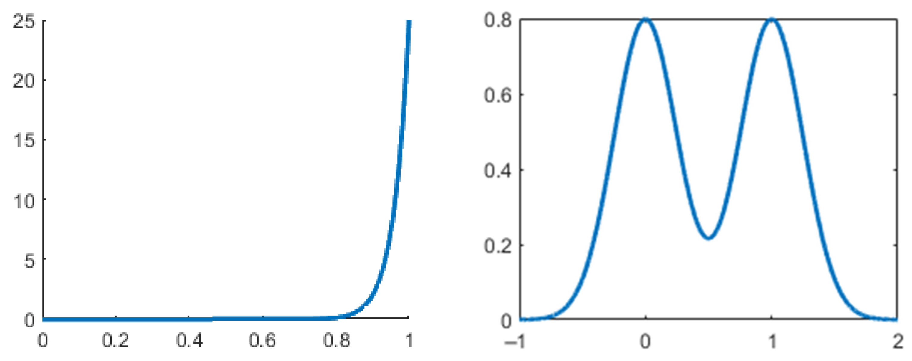
However, this test is not perfect. High values do not always indicate bimodality and low values do not always indicate non-bimodality. Figure 1 showcases this caveat with the unimodal beta distribution with probability density function (PDF) , and the bimodal binormal distribution with PDF , where and are the mixing weights. In practice, a common threshold for this coefficient is 0.555. Distributions with values greater than this are considered bimodal, and the ones with values lower than this are not. Knapp [18] compares the performance of this BC with the performance of other tests and shows a unimodal distribution for which the BC takes a very high value (0.78) compared to the actual bimodal distributions (0.56–0.66).
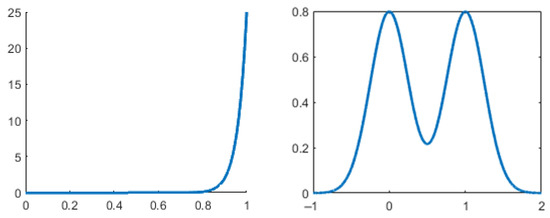
Figure 1.
Unimodal distribution (left) with high BC (0.8), and bimodal distribution (right) with low BC (0.58).
2.2. Fast Generation of Moments
The reason we are interested in bimodality tests that can be run in constant time is the development of applications that are dealing with large amounts of data and must partition or classify portions of data as fast as possible. Such an application may be one that binarizes a sample from an unknown n-dimensional signal by identifying, for each sample point, the best window for which to apply a specific threshold-based binarization algorithm (e.g., Otsu’s [22] method).
Sarle’s bimodality coefficient requires the computation of standardized moments 3 and 4 (skewness and kurtosis), which in turn require the computation of raw moment 1 and central moment 2 (mean and variance). However, the brute-force approach for these computations is of a linear order (), and the number of windows in the sample space is of a squared order (), resulting in the complexity of a cubed order (). Luckily, a constant order () approach for the in-window computations exists and is presented in the following subsections.
2.2.1. Summed-Area Table Technique
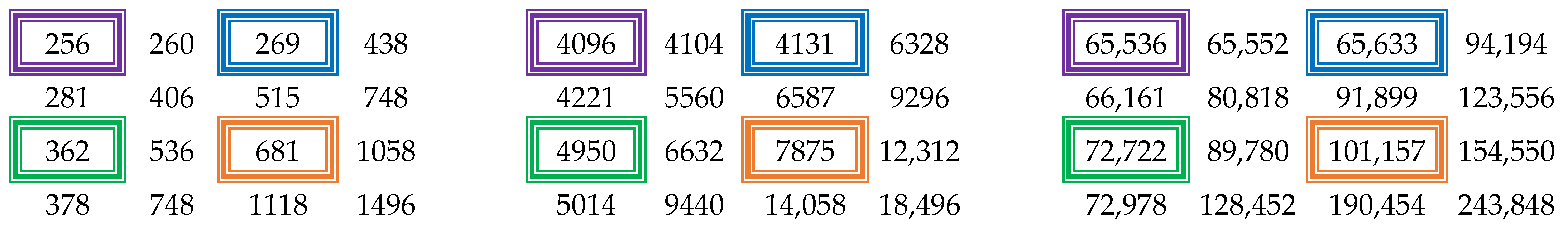
The mean of a window can be computed in constant time using a technique called the summed-area table [23]. The idea behind this is that by pre-computing the sums of the samples, the sum of a certain window can be computed as a function of the sums of the extremity points of the window. For a one-dimensional signal, the sum of a window would simply be the sum up to the point at the end of the window, minus the sum up to the point before the beginning of the window. Figure 2 shows how to compute the sum of a window for a two-dimensional signal. The sum of the window of interest (red) is equal to the sum of the orange window, whose value is stored in the summed-area table at the coordinates of the bottom right corner, plus the sum of the purple window (top left corner), minus the sum of the blue window (top right corner), minus the sum of the green window (bottom left corner). This technique can be applied to an n-dimensional signal for any natural number n.
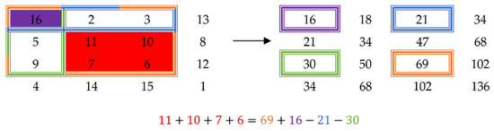
Figure 2.
Example of a summed-area table (right) obtained from a 2D matrix (left).
2.2.2. Generation of Moments Using Sums of Power
However, these sums divided by the number of samples in the window only yield the raw moments. Luckily, central, and standardized moments can be expressed as a function of raw moments of rank lower or equal to theirs as follows [24]:
where is the central moment of order n, and is the raw moment of order j and is the mean value of the distribution. Denoting as the standardized moment of order n, with representing the standard deviation of the distribution, we have the formula for Sarle’s BC as:
where . Applying the technique described in the previous section on the matrix in Figure 2, we can obtain the summed-area tables for higher powers, as illustrated in Figure 3.
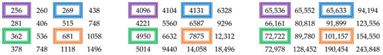
Figure 3.
Summed-area tables for higher powers: (left) 2nd, (middle) 3rd, (right) 4th.
2.3. Generalized Bimodality Coefficient (GBC)
Theorem 1.
Let X be a distribution,its central moments, andits standardized moments. Let
Then, the inequalityholds for any distribution, with equality only for distributions concentrated on two points.
Proof.
Let
Since is concave and all finite distributions with zero mean are (convex) mixtures of distributions concentrated on at most two points [25], the theorem will be proven if we can show that for all two-point distributions.
A two-point distribution takes the form Then where We can substitute this value in the equation we want to prove and find that:
which is equivalent to for all distributions concentrated on at most two points. □
2.4. Composite Bimodality Coefficient (CBC)
As previously shown, comparing a bimodality coefficient’s value to a set threshold is a weak test on its own. To have a strong test, we consider different formulas to mix our GBCs and obtain a CBC (see Appendix A). After running different tests with said formulas, we define our CBC according to a mixed power law, in the form seen in Equation (5):
This formula ensures that each GBC contributes to the test, and their respective powers represent the weight with which they do.
Since the problem at hand deals with a variety of possible distributions, potential mixtures of them, and imperfect data pertaining to said distributions, finding a set of powers that can be considered optimal in terms of general approximation is a difficult challenge. With that in mind, we found no way to analytically determine the best set of powers and thus resorted to the empirical method. We decided that a good way to establish the veracity of the CBC is by testing its performance in an image binarization application.
There are multiple ways to go about finding a set of powers that can fit a generic CBC. One that we tried initially was doing a simple grid-search using an image dataset, by starting around a series of points representing the powers of each GBC and shifting around them to increase the accuracy of our results. However, this method proved to be both lengthy and inefficient, as determining the accuracy of a set of powers in the image dataset took a while to compute (~10–20 min); given the thousands of possible combinations, the time to test them would increase to days. Subsequently, another factor that was an issue was that each new image that was added would change the order of the sets around, with the same one almost never being at the top again, whilst the accuracy of all sets was very similar to one another and within the margin of error. The third issue with this approach was that we do not know ahead of time whether a distribution is bimodal or not.
Thus, we needed a different approach that we could run on a dataset of known distributions in a fast time, obtain a set of powers on said dataset, and then run the CBC obtained by combining those powers against the original image dataset. For this purpose, we chose to train and use a very simple neural network, as the process for finding the desired values using one is very similar to that of a grid-search.
Our approach consisted of training a neural network to predict a potential set of powers that can be used in our composite coefficient. Since we were interested in obtaining a simple formula that can be applied in a fast, straightforward manner to compute values in real-time, we aimed to build a very rudimentary network configuration, more specifically that of a perceptron [26]. To determine a proper configuration for our network, we also considered the way the value of a node is computed, and the one-to-one relationship between the set of values that we wanted to find and our bimodality coefficients. Thus, we could build a straightforward network where our only output was represented by our CBC, and the inputs, associated with our GBCs, were directly connected to it.
Theorem 2.
Letrepresent the inputs of our network,the associated weights, and y the output of our network to which all the inputs are connected directly, with f(x) as its activation function and b as its activation bias. If
Proof.
Let
Something to be noted is that we chose to use only the first 3 GBCs in our approach, due to two reasons. First, as previously discussed, higher-order GBCs tend to be more error-prone to noise; thus, using them with a variety of distributions can potentially lead to poorer results. Secondly, computing higher-order GBCs requires a lot of resources to guarantee the precision necessary to store the values which can also take a lot of time, and is not the intended use for our coefficient that is meant to be fast and reliable. □
3. Preparing the Dataset for Training and Testing
For our training dataset, we chose to generate it from a variety of distributions, for two simple reasons. First, since we know the distributions involved in generating the data, we know ahead of time if a sample should follow a one or two-point focused distribution. Second, due to controlling the distributions involved in generating our samples, we can limit some of the caveats that were previously mentioned that negatively impact our GBC. For this purpose, we chose to generate random data points using twelve different distributions (see Appendix B), respectively a mixture of them, aimed at a variety of potential unimodal and bimodal results, generating a total of approximately 25,000 distributions. In a similar fashion, to vary the potential values of the GBCs pertaining to each distribution, we generated sets with a varying number of points, between 500 and 10,000. Because we wanted to test the veracity of the CBC in a binarization application, all values were generated in the interval , for an easier overall approach; however, this does not alter the result, as any distribution could be shifted and scaled to any other interval of choice, and the standardized central moments would not change.
After we generated the data, we computed the following for each set of points pertaining to a distribution: the moments, respectively the GBC from them, as well as a value that we would like our CBC to tend to for that set of points. We denoted these values as CBC’ and they will be used as the output of the network during the training step. Since we know the original distributions that generated our sets of points, we can compute CBC′ in two ways, depending on whether or not the original distribution was unimodal or bimodal:
For a bimodal distribution we denote with the position of the two modes of the distribution.
Theorem 3.
Let. Then.
Proof.
The last case for is similar to (14). From (11)–(14) we can see that . □
In the above equations, represents a correction factor based on the distance between the two modes of the distribution, such that two close modes do not give a high value for the CBC’. Similarly, is a normalization factor, typically chosen in the interval to ensure we always raise to subunit powers, and that can raise exponentially closer to 1 when the modes start spreading apart. The reason for using a correction factor is because a set of points generated by a bimodal distribution with two close modes would be almost indistinguishable from one generated by a unimodal distribution with a similar shape and with its mode lying somewhere between the two modes of the bimodal one. In a similar fashion, we used when the value of the PDF differs between the two nodes so that modes that are very spread vertically, but not horizontally, do not result in high CBC’ values.
3.1. Training the Network
Based on the previously computed values, we could train our network using the natural logarithms of GBCs as inputs and CBC’ as the output. However, before training our network, we also considered a second potential remap of our inputs, before applying our logarithmic function on the GBCs, one based on polynomial fitting (see Appendix C). This approach did lead to increased overall accuracy; thus, it was kept both for later training and testing purposes.
Since the training of the network was based on gradient descent, and we used a very simple network configuration, we had no certainty that our search would hit a global optimum, and, even if it did, we could not be sure of the general applicability of such an optimum. Consequently, since we did not know which set of powers might behave best in practice, we needed to obtain multiple sets and compare them. Thus, we trained different networks, with different constraints, such as using a different dataset when training, or constraining the weights, either to a set interval or simply making them strictly positive, to obtain our possible CBC parameters.
3.2. Testing the CBC
Tests were conducted against an image dataset generated by combining the following datasets: the DIBCO datasets [27,28,29,30,31,32,33,34,35], the PHIBD 2012 [36] dataset, the Nabuco dataset [37], and the Rahul Sharma dataset [38], the combination of which will be further denoted simply as the Images dataset. On this dataset, we ran a binarization algorithm starting from multiple possible choices, with various window sizes. We decided to settle on one based on Otsu’s method with a fixed 8 × 8 window size centered on each pixel. There were also separate tests conducted against a synthetic dataset obtained from random data pertaining to multiple distributions and mixtures of them.
4. Numerical Results
4.1. Accuracy of GBC
To quantify the accuracy, we used the F-measure (FM) defined as follows:
where TP stands for true positives, FP for false positives, and FN for false negatives. In Table 1, we can see the different F-measures associated with each GBC on both datasets. One thing to note is that higher-order GBCs tend to decrease in accuracy when trying to identify whether a distribution is bimodal or not, a point which will be discussed later as well as why higher-order GBCs might still be valuable, given certain scenarios.

Table 1.
F-measures of the first three GBCs.
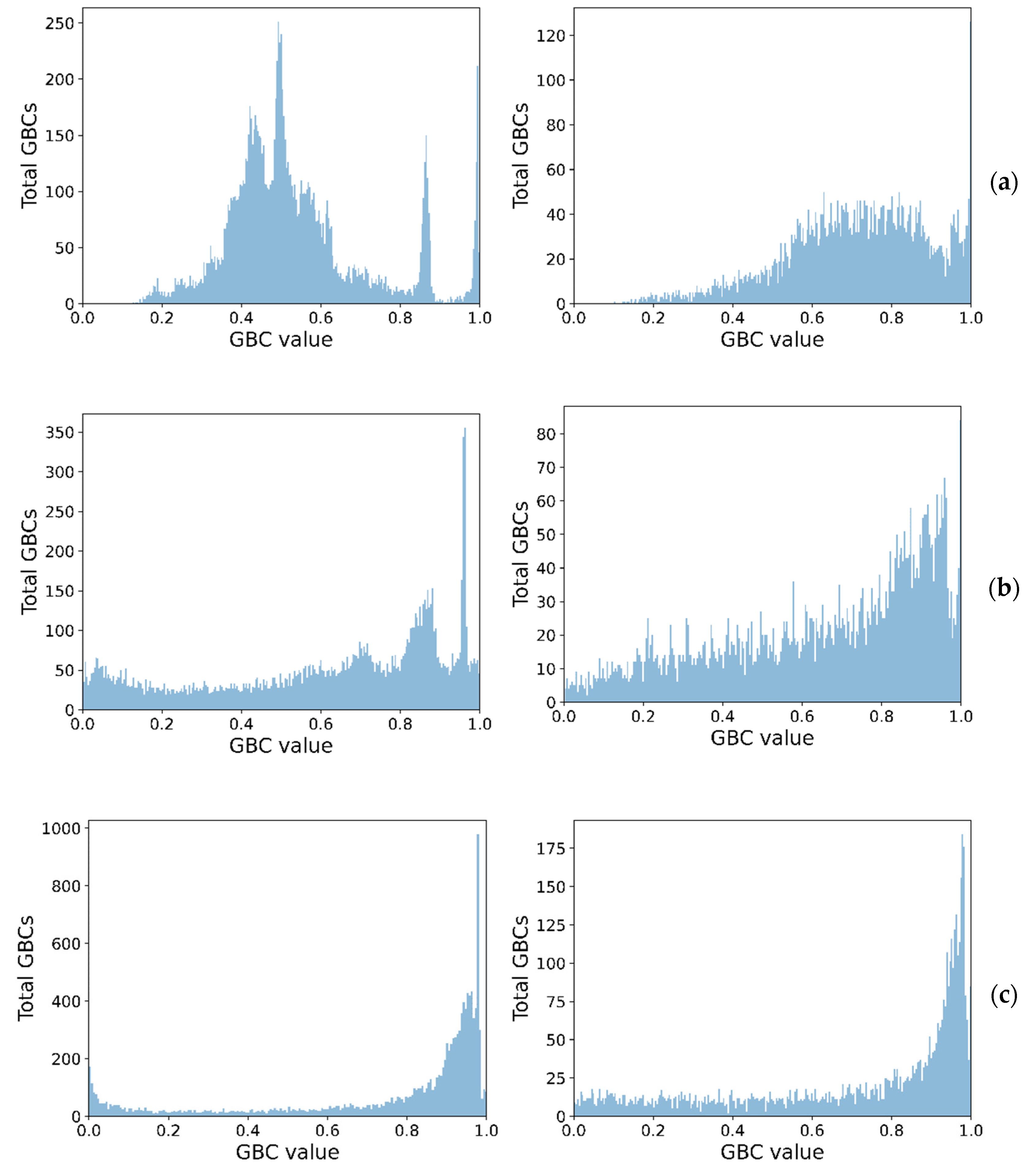
Figure 4 shows the class separation corresponding to each GBC, showing how higher-order GBCs tend to have their values more spread out, thus making it harder to pick a threshold. The peaks close to 1, for the unimodal cases, in all GBCs, are indicative of distributions with high skewness and low kurtosis, for the synthetic dataset.
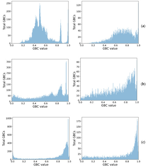
Figure 4.
Spread of GBC values for the two classes (unimodal left, bimodal right) on the synthetic dataset (a) GBC1, (b) GBC1, and (c) GBC3.
Table 2 shows the behaviors of the GBCs on a binormal distribution with varying means and variances. All of them decrease in values as the means get closer to each other and increase in value as the variances decrease, which indicates that they encourage bimodal distributions with more distinct peaks, with the higher-order GBCs being increasingly more sensitive. We compensated for the lower values of the higher-order GBCs by raising the powers of the lower-order GBCs.
Table 2.
Values for , , and for a binormal distribution with means , and variances , .
Table 3 shows the behaviors of the GBCs on a binormal distribution with fixed means and varying variances. The table is symmetrical, which indicates that they are insensitive to flipping transformations on the dataset.
Table 3.
Values for , , and for a binormal distribution with means , and variances , .
4.2. Accuracy of CBC
Table 4 shows some of the coefficients we ended up testing and their corresponding F-measures for both datasets. As we can see, just because a set of powers gives a good result for one dataset, does not necessarily mean it would do the same for the other, mostly due to the specific nature of the distributions that exist in each dataset. However, based on the overall performance, we would recommend the set of powers of either 3:2:1 or 3:0:1.
Table 4.
Mean values for F-measures for different power ratios.
5. Discussion
5.1. GBC Comparison with BC
As we could see from our results, higher order GBCs tend to be less accurate and less reliable as indices when identifying whether a distribution is bimodal or not. This is in part because of two reasons, the first being that higher order GBCs are more error-prone to noise, specifically because they require values that use higher powers for computation. The second thing to note is that it is harder to set a specific threshold at which to decide whether a distribution is bimodal or not, which could also be seen in our results.
However, this does not necessarily mean that using them in a composite coefficient is a bad thing. As we could see from the results pertaining to our CBC, it just means that using them individually can lead to worse results. However, for “well-behaved” distributions (low skewness, high kurtosis, and their respective higher-order moments), GBCs tend to have some benefits, when considering bimodal distributions:
- the higher the value of the two modes in a distribution, the higher the value of the GBC, with higher-order GBCs being more sensitive to this property;
- the more spread apart the two modes are, on the x-axis, the higher the value of the GBC, again, with higher-order GBCs being more sensitive;
- the closer the value of the two modes, on the y-axis, the higher the value of the GBC, where GBCs of higher-order behave better once again.
Something else to be noted is the fact that there is a huge jump when computing the F-measure for GBCs one and two on the Synthetic dataset, one of about 15; meanwhile, these values on the Images dataset tend to be very close together. This might be because the Synthetic dataset contains a lot of distributions with high skewness and low kurtosis, which, while they might make the dataset more generic, also have a negative influence on the results. Similarly, there is no guarantee that the set of synthetic distributions, or something close in nature to it, might exist in the real world. Thus, for future work, using sets that pertain to a more specific subset of distributions and mixtures of them, rather than such a large one, might be more beneficial.
5.2. CBC as a Bimodality Coefficient
As we could see from our results, the formula we used to compute our CBC gives better results, on both datasets we tested on, when compared to [18]. This does not mean that our coefficient is without issues, since distributions with high skewness and low kurtosis can still lead to misidentifying a unimodal distribution as a bimodal one.
A multitude of indices that were proposed [5,6,7,8,9] needs to make assumptions that the data they analyze fit a mixture of two normal distributions, which, often, is not necessarily the case. In this regard, from a generic point of view, our proposed coefficient can be more robust in some situations. A more significant advantage of our coefficient is its computational efficiency, especially when compared with the indices previously mentioned. Since we can compute the moments in a fast manner and we do not require to make assumptions or try to fit certain distributions to our data, we can determine in a fast and accurate manner whether some data fit a bimodal distribution or not. Table 5 shows the performance of our proposed coefficient, when using the powers 3:0:1, which compared with other indices, ran against a subsample of 4000 distributions of the Synthetic dataset. All tests were performed on an AMD Ryzen 9 5900HS processor. The times were averaged across 15 different runs of the program to address potential biases, whilst also looking for the best potential threshold for all indices, in order to maximize their F-measure, with the latter being a potential reason why a multitude of the indices shares the same F-measure.
Table 5.
Performance of different indices and methods on the Synthetic dataset.
Similarly, the computational efficiency of our coefficient can be seen when comparing it with the multitude of bimodality/multimodality tests proposed by [5,6,7,8,9,10]. Since most of these work directly on the histogram pertaining to a data sample, they tend to be slow, whilst also working with an uncertain stop condition, due to trying to find the best fit for said data. The indices proposed by the authors of [11,12] also work on the histogram, since they need to make approximations regarding the modes of the distribution. This can be both slow and can lead to poor results for bimodal distributions which have modes that are close together. Whilst our coefficient is not impervious to the closeness of the two modes, the fact that it is easier and faster to compute makes it more desirable.
Due to the fact that the image binarization test scenario is extremely complex, and running it on the Images dataset will result in an astonishing number of calls to any benchmarked bimodality coefficient (we counted about 300 million calls per sample from the Images dataset), it is unfeasible to run on the aforementioned dataset other coefficients that may be employed in Table 5 besides CBC, simply because they cannot be computed in constant time (O(1) complexity).
6. Conclusions
Determining whether some data follow a unimodal or bimodal distribution is an important step in figuring out a proper approach, in order to deal with said data, in a variety of situations. Thus, a proper way to ascertain this property is desired. A bimodality coefficient is a good starting point if it is robust.
In our case, the CBC performs better than any GBC on its own, for most of the composition ratios we tested, on average obtaining F-measure increases of 1.5–2%. However, finding an optimal ratio is no easy task, and even then, we have no certainty on how a CBC based on such a ratio might behave in more generic scenarios. For this reason, we also recommend two possible ratios to be considered: 3:2:1 and 3:0:1.
A certain downside of using the bimodality coefficient on its own is the fact that we do not know how data that follow a multimodal distribution with more than two modes behave. Thus, a multimodality coefficient could be considered for a better approach, and in future works, we could investigate ways to compute one.
Author Contributions
Conceptualization, N.T., M.-L.V. and C.-A.B.; Data curation, N.T., M.-L.V. and C.-A.B.; Formal analysis, N.T., M.-L.V. and C.-A.B.; Investigation, N.T., M.-L.V. and C.-A.B.; Methodology, N.T., M.-L.V. and C.-A.B.; Project administration, C.-A.B.; Resources, C.-A.B.; Software, N.T., M.-L.V. and C.-A.B.; Supervision, C.-A.B.; Validation, N.T., M.-L.V. and C.-A.B.; Visualization, N.T., M.-L.V. and C.-A.B.; Writing—original draft, N.T., M.-L.V. and C.-A.B.; Writing—review and editing, N.T., M.-L.V. and C.-A.B. All authors have read and agreed to the published version of the manuscript.
Funding
The APC has been supported by Politehnica University of Bucharest, through the PubArt program.
Institutional Review Board Statement
Not applicable.
Informed Consent Statement
Not applicable.
Data Availability Statement
Not applicable.
Conflicts of Interest
The authors declare no conflict of interest.
Appendix A
It is unreasonable to consider that a CBC comprised of a product of GBCs would yield the best results in practice. Thus, various other formulas were also considered as potential approaches for the problem at hand; however, none seemed to give many more beneficial results when considering both the results on the synthetic dataset of generated distributions or the image binarization dataset. Moreover, even when they did, it was very situational and only for a subset of the entire dataset. The F-measures for some of these formulas can be seen in Table A1, once again considering just the first three GBCs for practical reasons. These are not all the formulas we tested, but just some of those that we considered being more relevant in our case. The formulas are also presented without additional coefficients attached to our GBCs for simplicity. In practice, we tested both GBCs raised to different powers or multiplied with different coefficients.
Table A1.
Results for different formulas we experimented with.
Table A1.
Results for different formulas we experimented with.
| General Formula | Tested Formula | F-Measure (%) | Dataset |
|---|---|---|---|
| 76.953 | Images | ||
| 47.845 | Synthetic | ||
| 76.976 | Images | ||
| 47.138 | Synthetic | ||
| 65.513 | Images | ||
| 44.366 | Synthetic | ||
| 58.98 | Images | ||
| 64.69 | Synthetic | ||
| 58.98 | Images | ||
| 62.788 | Synthetic |
Appendix B
In order to generate a dataset both for training and testing our network, we chose to combine the following distributions: Beta [39,40], Burr [41,42], Exponential [43,44,45], Frechet [46,47,48], Gumbel [49,50], Laplace [51,52], Logistic [53,54], Log-Logistic [55,56,57], Log-Normal [58,59,60], Normal [61,62], Pareto [63,64], and Weibull [65,66]. Obviously, there are a lot more distributions that we could have used, but we considered these to be representative enough for our purposes. As can be seen, we chose to use only continuous distributions, as discrete ones would lead to similar results, with no additional benefits when generating the data itself.
Each distribution has a different set of parameters associated with it, that determines its shape. For non-mixed distributions, we simply chose these parameters randomly and generated the distribution and the random set of points based on it. For mixtures of distribution, in a similar fashion, we chose the two sets of parameters randomly, whilst also picking a scaling coefficient for each distribution that determined how much it contributed to the result. The sum of these scaling coefficients was one. Table A2 shows the set of these distributions as well as the parameters associated with each of them, and the values we considered for them, with . For some of these distributions, we skewed the selection of the parameters to certain intervals to obtain more representative distributions, with the probability of selecting the skewed interval for the parameters being denoted with p.
Table A2.
Distributions used in creating the Synthetic dataset.
Table A2.
Distributions used in creating the Synthetic dataset.
| Distribution | Parameters | |
|---|---|---|
| Beta | ||
| Burr | ||
| Exponential | ||
| Frechet | ||
| Gumbel | ||
| Laplace | ||
| Logistic | ||
| Log-Logistic | ||
| Log-Normal | ||
| Normal | ||
| Pareto | ||
| Weibull |
Appendix C
Something we also considered was using a function that could remap the value of our GBCs to better fit what we considered the “ideal” coefficient, CBC’, as described in Section 3. For these, we considered using a polynomial approximation. We tried polynomials of different degrees; however, polynomials of degrees higher than 3 would give values outside of the interval , for some GBCs in . Thus, even though they were fitting the data better at some points, since they were not robust for our purpose they were discarded and only degree 3 polynomials were considered. The formulas for the three polynomials used can be seen in Equations (A1)–(A3), where corresponds to .
Applying this conversion on the GBCs yielded better overall results, obtaining an F-measure of 65.025 on the 1:1:1 ratio, which was much higher than the initial 47.138, on the Synthetic dataset alone.
References
- Hartigan, J.A.; Hartigan, P.M. The Dip Test of Unimodality. Ann. Stat. 1985, 13, 70–84. [Google Scholar] [CrossRef]
- Silverman, B.W. Using Kernel Density Estimates to Investigate Multimodality. J. R. Stat. 1981, 43, 97–99. [Google Scholar] [CrossRef]
- Muller, D.W.; Sawitzki, G. Excess Mass Estimates and Tests for Multimodality. J. Am. Stat. Assoc. 1991, 86, 738–746. [Google Scholar] [CrossRef]
- Rozál, G.P.M.; Hartigan, J.A. The MAP Test for Multimodality. J. Classif. 1994, 11, 5–36. [Google Scholar] [CrossRef]
- Ashman, K.M.; Bird, C.M.; Zepf, S.E. Detecting Bimodality in Astronomical Datasets. Astron. J. 1994, 108, 2348–2361. [Google Scholar] [CrossRef] [Green Version]
- Zhang, C.; Mapes, B.; Soden, B. Bimodality in Tropical Water Vapor. Q. J. R. Meteorol. Soc. 2003, 129, 2847–2866. [Google Scholar] [CrossRef]
- Wang, J.; Wen, S.; Symmans, W.F.; Pusztai, L.; Coombes, K.R. The Bimodality Index: A Criterion for Discovering and Ranking Bimodal Signatures from Cancer Gene Expression Profiling Data. Cancer. Inform. 2009, 7, 199–216. [Google Scholar] [CrossRef] [Green Version]
- Bayramoglu, I. Bivariate and multivariate distributions with bimodal marginals. Commun. Stat. Theory Methods 2019, 49, 361–384. [Google Scholar] [CrossRef]
- Jammalamadaka, S.; Jin, Q. A Bayesian Test for the Number of Modes in a Gaussian Mixture. Asian, J. Stat. Sci. 2021, 1, 9–22. [Google Scholar]
- Chaudhuri, D.; Agrawal, A. Split-and-Merge Procedure for Image Segmentation Using Bimodality Detection Approach. Def. Sci. J. 2010, 60, 290–301. [Google Scholar] [CrossRef]
- Van Der Eijk, C. Measuring Agreement in Ordered Rating Scales. Qual. Quant. 2001, 35, 325–341. [Google Scholar] [CrossRef]
- Wilcock, P.R. Critical Shear Stress of Natural Sediments. J. Hydraul. Eng. 1993, 119, 491–505. [Google Scholar] [CrossRef]
- Smith, G.H.S.; Nicholas, A.P.; Ferguson, R.I. Measuring and Defining Bimodal Sediments: Problems and Implications. Water Resour. Res. 1997, 33, 1179–1185. [Google Scholar] [CrossRef]
- Contreras-Reyes, J.E. An asymptotic test for bimodality using the Kullback-Leibler divergence. Symmetry 2020, 12, 1013. [Google Scholar] [CrossRef]
- Vichitlimaporn, C.; Anantawaraskul, S.; Soares, J.B. Molecular Weight Distribution of Ethylene/1-Olefin Copolymers: Generalized Bimodality Criterion. Macromol. Theory Simul. 2017, 26, 1600060. [Google Scholar] [CrossRef]
- Hassanian-Moghaddam, D.; Moattari, M.M.; Rezania, A.; Sharif, F.; Ahmadi, M. Analytical representation of bimodality in bivariate distribution of chain length and chemical composition of copolymers. Chem. Eng. J. 2022, 431, 133229. [Google Scholar] [CrossRef]
- Voříšek, J. Estimation and bimodality testing in the cusp model. Kybernetika 2018, 54, 798–814. [Google Scholar] [CrossRef]
- Knapp, T. Bimodality Revisited. JMASM 2007, 6, 8–20. [Google Scholar] [CrossRef]
- Hildebrand, D.K. Kurtosis measures bimodality? Am. Stat. 1971, 25, 42–43. [Google Scholar]
- Shohat, J. Inequalities for moments of frequency functions and for various statistical constants. Biometrika 1929, 21, 361–375. [Google Scholar] [CrossRef]
- Pearson, K. Editorial note on the Limitation of Frequency Constants. Biometrika 1929, 21, 370–375. [Google Scholar]
- Otsu, N. A Threshold Selection Method from Gray-Level Histograms. IEEE Trans. Syst. Man Cybern. Syst. 1979, 9, 62–66. [Google Scholar] [CrossRef] [Green Version]
- Crow, F.C. Summed-Area Tables for Texture Mapping. In Proceedings of the 11th annual conference on Computer graphics and interactive techniques, Minneapolis, MN, USA, 23–27 July 1984; SIGGRAPH ’84. Association for Computing Machinery: New York, NY, USA, 1984; pp. 207–212. [Google Scholar] [CrossRef]
- Small, C.G. Expansions and Asymptotics for Statistics; Chapman and Hall/CRC: New York, NY, USA, 2010. [Google Scholar]
- Rohatgi, V.K.; Székely, G.J. Sharp Inequalities between Skewness and Kurtosis. Stat. Probab. Lett. 1989, 8, 297–299. [Google Scholar] [CrossRef]
- Rosenblatt, F. The Perceptron—A Perceiving and Recognizing Automaton; Techreport 85-460–1; Cornell Aeronautical Laboratory: Ithaca, NY, USA, 1957. [Google Scholar]
- Gatos, B.; Ntirogiannis, K.; Pratikakis, I. ICDAR 2009 Document Image Binarization Contest (DIBCO 2009). In Proceedings of the 2009 10th International Conference on Document Analysis and Recognition, Barcelona, Spain, 26–29 July 2009; pp. 1375–1382. [Google Scholar] [CrossRef]
- Pratikakis, I.; Gatos, B.; Ntirogiannis, K. H-DIBCO 2010—Handwritten Document Image Binarization Competition. In Proceedings of the 2010 12th International Conference on Frontiers in Handwriting Recognition, Kolkata, India, 16–18 November 2010; pp. 727–732. [Google Scholar]
- Pratikakis, I.; Gatos, B.; Ntirogiannis, K. ICDAR 2011 Document Image Binarization Contest (DIBCO 2011). In Proceedings of the 2011 International Conference on Document Analysis and Recognition, Beijing, China, 18–21 September 2011; pp. 1506–1510. [Google Scholar]
- Pratikakis, I.; Gatos, B.; Ntirogiannis, K. ICFHR 2012 Competition on Handwritten Document Image Binarization (H-DIBCO 2012). In Proceedings of the 2012 International Conference on Frontiers in Handwriting Recognition, Bari, Italy, 18–20 September 2012; pp. 817–822. [Google Scholar]
- Pratikakis, I.; Gatos, B.; Ntirogiannis, K. ICDAR 2013 Document Image Binarization Contest (DIBCO 2013). In Proceedings of the 2013 12th International Conference on Document Analysis and Recognition, Washington, DC, USA, 25–28 August 2013; pp. 1471–1476. [Google Scholar]
- Ntirogiannis, K.; Gatos, B.; Pratikakis, I. ICFHR2014 Competition on Handwritten Document Image Binarization (H-DIBCO 2014). In Proceedings of the 2014 14th International Conference on Frontiers in Handwriting Recognition, Hersonissos, Greece, 1–4 September 2014; pp. 809–813. [Google Scholar]
- Pratikakis, I.; Zagoris, K.; Barlas, G.; Gatos, B. ICFHR2016 Handwritten Document Image Binarization Contest (H-DIBCO 2016). In Proceedings of the 2016 15th International Conference on Frontiers in Handwriting Recognition (ICFHR), Shenzhen, China, 23–26 October 2016; pp. 619–623. [Google Scholar]
- Pratikakis, I.; Zagoris, K.; Barlas, G.; Gatos, B. ICDAR2017 Competition on Document Image Binarization (DIBCO 2017). In Proceedings of the 2017 14th IAPR International Conference on Document Analysis and Recognition (ICDAR), Kyoto, Japan, 9–15 November 2017; pp. 1395–1403. [Google Scholar]
- Pratikakis, I.; Zagoris, K.; Karagiannis, X.; Tsochatzidis, L.; Mondal, T.; Marthot-Santaniello, I. ICDAR 2019 Competition on Document Image Binarization (DIBCO 2019). In Proceedings of the 2019 International Conference on Document Analysis and Recognition (ICDAR), Sydney, Australia, 20–25 September 2019; pp. 1547–1556. [Google Scholar]
- Nafchi, H.Z.; Ayatollahi, S.M.; Moghaddam, R.F.; Cheriet, M. Persian Heritage Image Binarization Dataset (PHIBD 2012), ID: PHIBD 2012_1. Available online: http://tc11.cvc.uab.es/datasets/PHIBD 2012_1 (accessed on 20 March 2022).
- Lins, R.D. Two Decades of Document Processing in Latin America. J. Univers. Comput. Sci. 2011, 17, 151–161. [Google Scholar]
- Singh, B.M.; Sharma, R.; Ghosh, D.; Mittal, A. Adaptive binarization of severely degraded and non-uniformly illuminated documents. Int. J. Doc. Anal. Recognit. 2014, 17, 393–412. [Google Scholar] [CrossRef]
- Ma, Z.; Leijon, A. Beta Mixture Models and the Application to Image Classification. In Proceedings of the 2009 16th IEEE International Conference on Image Processing (ICIP), Cairo, Egypt, 7–10 November 2009; pp. 2045–2048. [Google Scholar] [CrossRef]
- Gupta, A.K.; Nadarajah, S. Beta Function and the Incomplete Beta Function. In Handbook of Beta Distribution and Its Applications, 1st ed.; CRC Press: Boca Raton, FL, USA, 2004; pp. 3–32. [Google Scholar]
- Nadarajah, S.; Pogány, T.; Saxena, R. On the Characteristic Function for Burr Distributions. Statistics 2011, 46, 419–428. [Google Scholar] [CrossRef]
- Ahmad, K.; Jaheen, Z.; Mohammed, H. Finite Mixture of Burr Type XII Distribution and Its Reciprocal: Properties and Applications. Stat. Pap. 2011, 52, 835–845. [Google Scholar] [CrossRef]
- Gupta, A.K.; Zeng, W.-B.; Wu, Y. Exponential Distribution. In Probability and Statistical Models: Foundations for Problems in Reliability and Financial Mathematics; Gupta, A.K., Zeng, W.-B., Wu, Y., Eds.; Birkhäuser: Boston, MA, USA, 2010; pp. 23–43. [Google Scholar] [CrossRef]
- Elfessi, A.; Reineke, D. A Bayesian Look at Classical Estimation: The Exponential Distribution. J. Stat. Educ. 2001, 9. [Google Scholar] [CrossRef]
- Rather, N.; Rather, T. New Generalizations of Exponential Distribution with Applications. J. Probab. Stat. 2017, 2017, 2106748. [Google Scholar] [CrossRef] [Green Version]
- Nadarajah, S.; Pogány, T. On the Characteristic Functions for Extreme Value Distributions. Extremes 2013, 16, 27–38. [Google Scholar] [CrossRef]
- Gusmão, F.; Ortega, E.; Cordeiro, G. The Generalized Inverse Weibull Distribution. Stat. Pap. 2011, 52, 591–619. [Google Scholar] [CrossRef]
- Khan, M.S.; Pasha, G.; Pasha, A. Theoretical Analysis of Inverse Weibull Distribution. WSEAS Trans. Math. 2008, 7, 30–38. [Google Scholar]
- Gumbel, E.J. Les valeurs extrêmes des distributions statistiques. Ann. L’institut Henri Poincaré 1935, 5, 115–158. [Google Scholar]
- Evin, G.; Merleau, J.; Perreault, L. Two-Component Mixtures of Normal, Gamma, and Gumbel Distributions for Hydrological Applications. Water Resour. Res. 2011, 47. [Google Scholar] [CrossRef]
- Ding, P.; Blitzstein, J. On the Gaussian Mixture Representation of the Laplace Distribution. Am. Stat. 2017, 72, 172–174. [Google Scholar] [CrossRef]
- Eltoft, T.; Kim, T.; Lee, T.-W. On the Multivariate Laplace Distribution. IEEE Signal Process. Lett. 2006, 13, 300–303. [Google Scholar] [CrossRef]
- Decani, J.S.; Stine, R.A. A Note on Deriving the Information Matrix for a Logistic Distribution. Am. Stat. 1986, 40, 220–222. [Google Scholar] [CrossRef]
- Kumar, C.S. A Note on Logistic Mixture Distributions. Biom. Biostat. Int. J. 2017, 2, 122–124. [Google Scholar] [CrossRef] [Green Version]
- Ekawati, D.; Warsono, W.; Kurniasari, D. On the Moments, Cumulants, and Characteristic Function of the Log-Logistic Distribution. IPTEK J. Sci. 2015, 25. [Google Scholar] [CrossRef] [Green Version]
- Makubate, B.; Oluyede, B.; Dingalo, N.; Fagbamigbe, A. The Beta Log-Logistic Weibull Distribution: Model, Properties and Application. Int. J. Stat. Prob. 2018, 7, 49. [Google Scholar] [CrossRef]
- Oluyede, B.; Foya, S.; Warahena-Liyanage, G.; Huang, S. The Log-Logistic Weibull Distribution with Applications to Lifetime Data. Austrian J. Stat. 2016, 45, 43. [Google Scholar] [CrossRef]
- Zhang, X.; Barnes, S.; Golden, B.; Myers, M.; Smith, P. Lognormal-Based Mixture Models for Robust Fitting of Hospital Length of Stay Distributions. ORHC 2019, 22, 100184. [Google Scholar] [CrossRef]
- Sultan, K.; Al-Moisheer, A. Mixture of Inverse Weibull and Lognormal Distributions: Properties, Estimation, and Illustration. Math. Probl. 2015, 2015, 526786. [Google Scholar] [CrossRef]
- Yang, M. Normal Log-Normal Mixture, Leptokurtosis and Skewness. Appl. Econ. 2008, 15, 737–742. [Google Scholar] [CrossRef]
- Negarestani, H.; Jamalizadeh, A.; Shafiei, S.; Balakrishnan, N. Mean Mixtures of Normal Distributions: Properties. Metrika 2019, 82, 501–528. [Google Scholar] [CrossRef]
- Wang, J.; Taaffe, M. Multivariate Mixtures of Normal Distributions: Properties, Random Vector Generation, Fitting, and as Models of Market Daily Changes. INFORMS J. Comput. 2015, 27, 193–203. [Google Scholar] [CrossRef]
- Arnold, B.C. Pareto and Related Heavy-Tailed Distributions. In Pareto Distributions, 2nd ed.; Chapman and Hall/CRC: London, UK, 2015; pp. 41–115. [Google Scholar]
- Paduthol, S.; Nair, M. On a Finite Mixture of Pareto Distributions. CSAB 2005, 57, 67–84. [Google Scholar] [CrossRef]
- Mohammed, Y.; Yatim, B.; Ismail, S. A Parametric Mixture Model of Three Different Distributions: An Approach to Analyse Heterogeneous Survival Data. In Proceedings of the 21st National Symposium on Mathematical Sciences, Penang, Malaysia, 6–8 November 2013; Volume 1605. [Google Scholar] [CrossRef] [Green Version]
- Jiang, R.; Murthy, D.N.P. A Study of Weibull Shape Parameter: Properties and Significance. Reliab. Eng. 2011, 96, 1619–1626. [Google Scholar] [CrossRef]

Publisher’s Note: MDPI stays neutral with regard to jurisdictional claims in published maps and institutional affiliations. |
© 2022 by the authors. Licensee MDPI, Basel, Switzerland. This article is an open access article distributed under the terms and conditions of the Creative Commons Attribution (CC BY) license (https://creativecommons.org/licenses/by/4.0/).