Estimation of Parameters of Different Equivalent Circuit Models of Solar Cells and Various Photovoltaic Modules Using Hybrid Variants of Honey Badger Algorithm and Artificial Gorilla Troops Optimizer

Abstract

Parameters of the solar cell equivalent circuit models have a significant role in assessing the solar cells’ performance and tracking operational variations. In this regard, estimating solar cell parameters is a difficult task because cells have nonlinear current-voltage characteristics. Thus, a fast and accurate optimization algorithm is usually required to solve this engineering problem effectively. This paper proposes two hybrid variants of honey badger algorithm (HBA) and artificial gorilla troops optimizer (GTO) to estimate solar cell parameters. The proposed algorithms minimize the root mean square error (RMSE) between measurement and simulation results. In the first variant, GTO is used to determine the initial population of HBA, while in the second variant, HBA is used to determine the initial population of GTO. These variants can efficiently improve convergence characteristics. The proposed optimization algorithms are applied for parameter estimation of different equivalent circuit models of solar cells and various photovoltaic (PV) modules. Namely, the proposed algorithms test three solar cell equivalent models: single-diode, double-diode, and triple-diode equivalent circuit models. Different photovoltaic modules are investigated, such as the RadioTechnique Compelec (RTC) France solar cell, Solarex’s Multicrystalline 60 watts solar module (MSX 60), and the Photowatt, France solar panel (Photo-watt PWP 201). In addition, the applicability of the proposed optimization algorithms is verified using obtained results from a commercial solar module called Shell Monocrystalline PV module (SM55) with different irradiation and temperature levels. The good results of the proposed algorithms show that they can efficiently improve convergence speed and the accuracy of the obtained results than other algorithms used for parameter estimation of PV equivalent circuit models in the literature, particularly in terms of the values of the RMSE and statistical tests. In addition, the parameters estimated by the proposed methods fit the simulation data perfectly at different irradiance and temperature levels for the commercial PV module.

1. Introduction

The transmission and distribution systems in modern power systems represent vital links in the power supply chain. Unlike a transmission system that consists of a small number of significant components, a distribution system includes a large number of small elements, which increases the complexity of the supervision and control of this system. With the growing dependence of society and economy on electricity, the transmission and the distribution systems need to ensure an acceptable level of reliability, quality, and security of electricity supply in the most economically efficient way. The power system is going through a dynamic transition. Reducing carbon dioxide (CO₂) emissions requires reliance on renewable energy sources (RESs) to drastically reduce or even eliminate the use of coal in energy production. These days, power systems involve an increasing number of components that rely on power-electronic elements, such as energy storage systems, reactive energy compensation systems, electric vehicles, etc. These additional components are essential for regulating power, losses, and voltage deviations [1].

RESs such as solar and wind energy resources mainly depend on geographic location, air temperature, and climate-related factors such as time of day, season, wind speed, level of direct sunlight, pressure gradient, and others [2,3]. The use of RESs in transmission and distribution systems is increasing worldwide, further complicating power systems operation because RESs are characterized by an intermittent and unpredictable nature, which significantly complicates the management of these systems [4,5].

In European electricity markets, fuel prices represent a large share of the electricity prices. Although RESs can provide flexibility in the market, frequently, renewable electricity may not be consumed in the domestic market due to insufficient national network capacity. Consequently, electricity flows are pushed to grids of neighboring countries, resulting in recurring and severe congestion problems that also affect continuously-based or discretely-based intraday markets [6,7].

Renewable energy is the fastest-growing energy source in the United States (U.S.), with solar generation (including solar distributed generation) accounting for 3.3% of total U.S. generation in 2020 [8,9]. In this context, many countries, such as Egypt and Saudi Arabia, provide incentives for the use of solar PV systems to enable a powerhouse for growth in renewable electricity. However, the proper and efficient use of solar PV requires voltage and current regulation systems to maintain power at the maximum power point (MPP). Because of this, modeling, analysis and testing of current-voltage characteristics of solar cells are essential, and this is confirmed by many publications that deal with modeling and estimating the parameters of equivalent circuit models of solar cells.

Three equivalent circuit models of solar cells, which differ in the number of diodes, are commonly used in the literature. The simplest and most widely used solar model is the single-diode model (SDM) [3,10]. It is a model represented by a single current source (representing the photo-current), a diode connected in parallel to the current source, a parallel-connected resistor, and a series-connected resistor. As the diode is modeled with two unknown parameters, this model is described with five unknown parameters [11]. To increase the model’s accuracy, a parallel-connected diode is added in the double-diode model (DDM), and two parallel-connected diodes are added in the triple-diode model (TDM). Thus, the two-diode model is described with seven unknown parameters, and the three-diode model is described with nine unknown parameters. These models’ accuracy is higher than the accuracy of SDMs [12].

Determining the unknown parameters of solar cells is a challenging scientific problem. Today, many approaches, algorithms, and methods can estimate parameters of different equivalent circuit models of solar cells and PV modules. Solar panel manufacturers generally provide nominal irradiance and temperature data associated with values of open-circuit voltage, short-circuit current, and current at maximum power. The parameter estimation of equivalent circuit models of solar cells can be performed based on manufacturer’s data [3]. However, the manufacturer’s data do not provide sufficient information for complete and accurate modeling of solar cells, mainly due to unsung resistors data. Thus, it is necessary to use analytical, numerical or metaheuristic-based methods to estimate unknown parameters of solar cells equivalent circuit models using measured voltage-current data. Unfortunately, these methods require solving transcendental nonlinear equations.

Numerical methods such as Newton and Levenberg–Marquardt-based methods can be used for parameter estimation. However, these methods depend on the initial values of the parameters, require many iterations to obtain an acceptable solution, and do not usually converge towards a global solution [10]. These are the main reasons for the application of metaheuristic methods to estimate parameters of equivalent circuit models of solar cells.

Nowadays, many algorithms are used to estimate parameters of equivalent circuit models of solar cells. These algorithms can be divided into several groups based on their inspiration processes or implemented methods; for instance, a group of bio-inspired algorithms (BIA) that are inspired by biological processes in nature and includes genetic algorithms based on non-uniform mutation (GAMNU) [13], bee pollinator flower pollination algorithm (BPFPA) [14], memetic adaptive differential evolution (MADE) [15], and improved shuffled complex evolution (ISCE) [16]. Additionally, a group of socially-oriented algorithms that are inspired by describing the behavior of people and children under specific situations have emerged. A group of socially-oriented algorithms inspired by teaching–learning behaviour of people and children has also emerged. This group includes the gaining–sharing knowledge-based algorithm (GSK) [17], teaching-learning-based optimization (TLBO) and improved TLBO (ITLBO) [18], and teaching–learning-based artificial bee colony (TLABC) [19]. Another group includes algorithms that rely on natural physical processes, such as water movement, earth movement, and others, such as the wind-driven optimization (WDO) algorithm [20]. A group of algorithms inspired by the behavior and lifestyle of animals and birds has also developed. This group includes the Whippy Harris hawks optimization algorithm (WHHO) [21], cat swarm optimization (CSO) [22], modified particle swarm optimization (MPSO) [23], artificial bee colony (ABC) [24] and marine-predators algorithm (MPA) [25] algorithms. Besides, as many processes have a chaotic nature, many chaotic algorithms are often developed by adding chaotic variations to some algorithms, such as the chaotic optimization approach (COA) [26], chaotic successful history-based adaptive differential evolution variants with linear population size reduction algorithm (CLSHADE) [12], and chaotic gradient-based optimization (CGBO) with chaotic drifts [27]. Finally, a group of algorithms relies on hybridizing two or more algorithms to enhance their performance in finding global solutions [28,29]. The main advantage of the hybrid algorithms is their better proximity to global solutions than standard algorithms. Moreover, these algorithms require a small number of iterations to get the optimal solution. Moreover, hybridization of algorithms uses exploration and exploitation features of each algorithm, which significantly improves the quality of solutions that can be obtained.

The subject of research in this paper is two-fold. The first goal is to propose a new hybrid metaheuristic algorithm for efficiently estimating parameters of different equivalent circuit models of solar cells and PV modules. In this regard, two hybridization variants that rely on the honey badger algorithm (HBO) [30] and the artificial gorilla troops optimizer (GTO) [31] are proposed. The second goal is to estimate the accuracy of parameters of SDM, DDM, and TDM of well-known solar cells and modules presented in the literature to compare the obtained results with numerous results in the literature.

The main advantages of this research are outlined as follows:

• A new metaheuristic algorithm for estimating parameters of equivalent circuit models of solar cells and PV modules has been proposed.
• Two types of hybridization of algorithms used have been proposed.
• Statistical analysis of the results of these algorithms is examined.
• Performance of the proposed algorithms is compared with several well-known algorithms used in parameter estimation problems.
• The three equivalent circuit models of solar cells are addressed and investigated.
• The applicability and efficiency of the proposed methods are tested on commercial PV modules for different levels of temperature and irradiance.

The rest of the paper is organized as follows. In Section 2, a short review of the solar cell models is introduced. The description of the novel hybrid algorithm is presented in Section 3. Numerical results are shown in Section 4. In Section 5, the efficiency of the proposed algorithms for a commercial photovoltaic model, known as monocrystalline SM55 (SM55), is verified, whose current-voltage curves measured for different levels of irradiance and temperature were obtained from the manufacturer’s datasheet. The main contributions of this work and future work directions are given in Section 6.

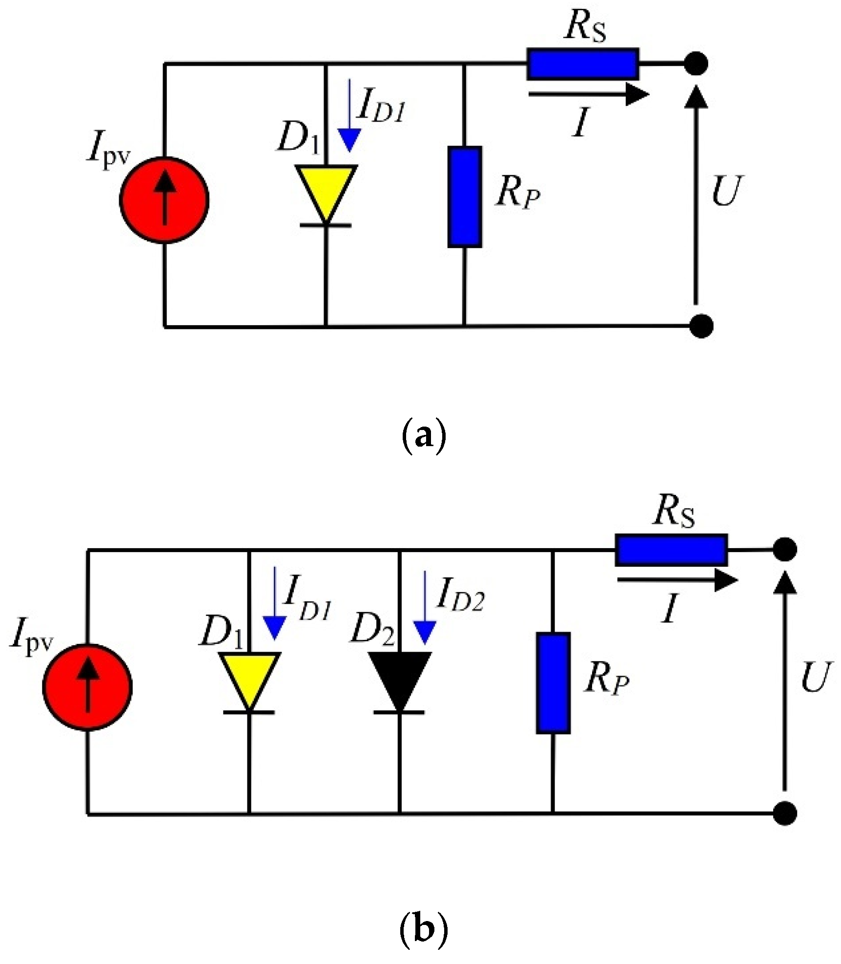
2. Solar Cell Equivalent Circuits

The simplest equivalent circuit of a solar PV cell consists of an ideal current source (I_pv) and a parallel-connected diode (D) [32,33,34,35,36,37,38,39]. The current of the ideal current source is directly proportional to the light flux to which the solar cell is exposed. The construction of the solar cell itself is a p-n junction. However, if one wants to consider the losses of solar cells, in that case, the previous model is supplemented with two resistances, one resistance is connected in parallel to the diode (R_P), and the other resistance is connected in series (R_S) with the diode. The equivalent circuit represents a five-parameter single-diode model (SDM) of a solar cell, shown in Figure 1a. This model is the most widely recognized model of solar cells. Its mathematical relation for current and voltage has the following form [40,41,42,43,44,45,46,47,48,49,50,51,52,53,54,55,56]:

$$I=I_{pv}-I_{01}\left(exp\left(\frac{U+I{R}_S}{n_1{V}_{th}}-1\right)-\frac{U+I{R}_S}{R_P}\right)$$

(1)

where I₀₁ denotes the reverse saturation current, n₁ represents the ideality factor, and V_th is the thermal voltage, and it equals K_BT/q, in which K_B is Boltzmann constant, T is the temperature in Kelvin, and q is the electron charge.

The analytical solution of current as a function of voltage for SDM of solar cells is given as follows [11]:

$$I=\frac{R_P\left(I_{pv}+I_0\right)-U}{R_S+R_P}-\frac{n_1{V}_{th}}{R_S}·W\left(\frac{I_{01}{R}_P{R}_S}{n_1{V}_{th}\left(R_S+R_P\right)}exp\left(\frac{R_P\left(R_S{I}_{pv}+R_S{I}_{01}+U\right)}{n_1{V}_{th}\left(R_S+R_P\right)}\right)\right)$$

(2)

In addition, the analytical solution of voltage as a function of current is given in (3).

$$U=\left(I_{pv}+I_{01}\right)R_P-I\left(R_S+R_P\right)-n_1{V}_{th}W\left(\frac{I_{01}{R}_P}{n_1{V}_{th}}exp\left(\frac{R_P\left(I_{pv}+I_{01}-I\right)}{n_1{V}_{th}}\right)\right)$$

(3)

In the five-parameter SDM, current and voltage can be expressed in terms of the Lambert W function, where W denotes the solution of the Lambert equation. In mathematics, the Lambert W function is a set of multivalued functions that are formulated as x = ϑ exp(−x), where its solution can be expressed in the form x = W(ϑ) [11,12]. Lambert W function can be solved using iterative-based methods or analytically using Taylor series or special trans function theory [57]. It should be mentioned that many mathematical programs such as Matlab, Mathematica and Maple have embedded solvers that can solve Lambert W functions.

An additional diode is added in DDM, and two other diodes are added in TDM. Therefore, the DDM is characterized by seven unknown parameters, while the TDM is characterized by nine unknown parameters. These models’ accuracy is higher than the accuracy of SDM [11,12]. The seven-parameter DDM and nine-parameter TDM of PV equivalent circuits are shown in Figure 1b,c, respectively.

The mathematical expressions of current and voltage for DDM and TDM have the forms given in (4) and (5), respectively. In these equations, I₀₂ and I₀₃ denote the reverse saturation currents of the second and third diodes, while n₂ and n₃ represent the second and third solar cells’ ideality factors, respectively.

$$I=I_{pv}-I_{01}\left(e^{\frac{U+I{R}_S}{n_1\times V_{th}}}-1\right)-I_{02}\left(e^{\frac{U+I{R}_S}{n_2\times V_{th}}}-1\right)-\frac{U+I{R}_S}{R_P}$$

(4)

$$I=I_{pv}-I_{01}\left(e^{\frac{U+I{R}_S}{n_1\times V_{th}}}-1\right)-I_{02}\left(e^{\frac{U+I{R}_S}{n_2\times V_{th}}}-1\right)-I_{03}\left(e^{\frac{U+I{R}_S}{n_3\times V_{th}}}-1\right)-\frac{U+I{R}_S}{R_P}$$

(5)

Equations (4) and (5) are transcendental equations that cannot be solved analytically [11,12] because of the high nonlinearity of the current expressions of these models. Thus, an iterative procedure is needed to solve them. In [12], expressions of current as a function of voltage are given for DDM and TDM, respectively, as follows:

$$I=\frac{R_p}{R_p+R_s}\left(I_{pv}+I_{01}+I_{02}-\frac{U}{R_P}-\frac{n_1{V}_{th}}{R_s}\left(1+\frac{R_s}{R_p}\right)\cdot \Psi \right)$$

(6)

$$I=\frac{R_p}{R_p+R_s}\left(I_{pv}+I_{01}+I_{02}+I_{03}-\frac{U}{R_P}-\frac{n_1{V}_{th}}{R_s}\left(1+\frac{R_s}{R_p}\right)\cdot \Psi \right)$$

(7)

where the variable Ψ represents the solution of the transcendent equations of DDM (Equation (8)) and TDM (Equation (9)). The constants${\alpha }_{TDM}$, ${\alpha }_{DDM}$, ${\beta }_{TDM}$, ${\beta }_{DDM}$, ${\delta }_{TDM}$, ${\delta }_{DDM}$, ${\gamma }_{TDM}$, and ${\sigma }_{TDM}$ rely on the parameters of the PV equivalent circuit models. The expressions describing these constants are given in the Appendix A at the end of the paper. Besides, readers can refer to [12] for detailed derivations of solutions of (6) and (7).

$${\alpha }_{DDM}+{\beta }_{DDM}·exp\left(\Psi ·{\delta }_{DDM}\right)=\Psi ·exp\left(\Psi \right)$$

(8)

$${\alpha }_{TDM}+{\beta }_{TDM}·exp\left(\Psi ·{\delta }_{TDM}\right)+{\gamma }_{TDM}·exp\left(\Psi ·{\sigma }_{TDM}\right)=\Psi ·exp\left(\Psi \right)$$

(9)

3. Proposed Hybrid Algorithms

Metaheuristic algorithms are among the most popular techniques for solving engineering optimization problems because of their effectiveness and ability to converge to global/semi-global solutions. Generally, metaheuristic algorithms have sets of potential solutions to the optimization problem. Each solution is iteratively updated following a specific procedure based on the nature of the algorithm. However, these algorithms are characterized by their stochastic nature because the population of solutions in the first iteration are randomly initialized between specific limits [5,58,59]. In this regard, the starting initial point has a significant impact on the convergence speed of the algorithm. To overcome this disadvantage, two new metaheuristic algorithms are proposed in this work. The algorithms proposed in this paper rely on the hybridization of two recently developed metaheuristic algorithms (honey badger algorithm (HBA) [30] and artificial gorilla troops optimizer (GTO) [60]). The first proposed algorithm is called GTO-HBA, and it used HBA to be the main algorithm whose initial population is determined using the GTO algorithm. The second proposed algorithm is called HBA-GTO, and it uses HBA to initialize the population of the GTO algorithm, instead of the random initialization. Therefore, the best possible starting point, i.e., population in the first iteration, would be obtained because the proposed algorithms depend on executing the algorithms one after another while benefiting from the exploration and exploitation capabilities of each algorithm. Further, the obtained population is sorted based on the value of the fitness function of each individual. The best individual that has the minimum fitness function value is chosen.

HBA imitates honey badger’s behaviour when locating food sources. Mathematically, each badger in the population is represented by its position x_i = [x_i¹, x_i², …, x_i^D], where D denotes the number of variables, and i = 1, 2, 3,..., N, and N stands for population size. The main equations repeated in HBA are the digging and honey phases. These equations are employed to update the positions of honey badgers.

The digging phase is expressed as follows:

$$x_{new}=x_{prey}+F\cdot \beta \cdot I\cdot x_{prey}+F\cdot r_3\cdot \alpha \cdot d_i\left|cos\left(2\pi r_4\right)\left[1-cos\left(2\pi r_5\right)\right]\right|$$

(10)

where x_new denotes the updated position of the honey badger, x_prey is the best badger obtained so far, β denotes the ability of the honey badger to get food (selected to be 6 in this work), and r₃, r₄, and r₅ are random numbers between 0 and 1. The smell intensity of the prey I_i, source strength S, distance between the prey and ith badger d_i, density factor α, and flag F, are expressed as follows:

$$I_i=r_2\left(\frac{S}{4\pi d_i^2}\right)$$

(11)

$$S={\left(x_i-x_{i+1}\right)}^2$$

(12)

$$d_i=x_{prey}-x_i$$

(13)

$$\alpha =exp\left(-\frac{t}{t_{max}} \right)$$

(14)

$$F=\{\begin{array}{c}1, if r_6\le 0.5 \\ -1, else \end{array}$$

(15)

where t stands for the current iteration, t_max is the maximum number of iterations, and r₂ and r₆ are random numbers with the range [0, 1].

The honey phase occurs when the honey badger follows the honey guide bird, and it is represented by (16).

$$x_{new}=x_{prey}+F{r}_1\alpha d_i$$

(16)

where r₁ denotes a random number with the range [0, 1].

Finally, the position of the honey badger (individual) with the lowest fitness function value represents the final solution obtained by HBA.

GTO algorithm is inspired by behavior of gorillas. Like HBA, each gorilla in the population represents the potential solution to the optimization problem.

In each iteration, the exploration phase comes first and is represented by (17):

$$X\left(t+1\right)=\{\begin{array}{c}\left(UB-LB\right)y_1+LB, rand<p\\ \left(y_2-C\right)X_r\left(t\right)+LH, rand\ge 0.5\\ X\left(i\right)-L\left(L\left(X\left(t\right)-G{X}_r\left(t\right)\right)+y_3\left(X\left(t\right)-G{X}_r\left(t\right)\right)\right), rand<0.5\end{array}$$

(17)

GX(t + 1) and X(t) represent the vectors of gorilla positions in the current and next iterations, respectively. The parameter p explores the probability of choosing an exploration strategy to an unidentified position and must be in the range [0, 1], while rand, y₁, y₂, and y₃ are random numbers range between 0 and 1. The parameters X_r(t) and GX_r(t) stand for randomly chosen gorillas from populations X and GX, respectively. The variables C, L, and H, can be calculated as follows:

$$C=F\left(1-\frac{t}{t_{max}}\right)$$

(18)

$$F=\cos \left(2y_4\right)+1$$

(19)

$$L=C·l$$

(20)

$$H=ZX\left(t\right)$$

(21)

where y₄ is a random number with the range [0, 1], l is a random number with the range [−1, 1], while Z is a random number with the range [−C, C]. At the end of exploration, the fitness function of all GX solutions is calculated. If the cost of GX(t) < X(t), then the GX(t) gorilla will replace X(t) solution. The best solution is the gorilla whose fitness function value has the lowest value (Silverback). Further, the exploitation phase comes after the exploration phase. It is mainly controlled by the parameter W that needs to be set at the beginning of the procedure. Depending on the value of C, vector GX(t + 1) is calculated according to the following relations:

$$GX\left(t+1\right)=\{\begin{array}{c}LM\left(X\left(t\right)-X_{siverback}\right)+X\left(t\right), if C\ge W\\ X_{silverback}-\left(X_{silverback}Q-X\left(t\right)Q\right)A, if C<W\end{array}$$

(22)

where the variable M can be calculated as follows in terms of population size (N), and g, which equals 2^L.

$$M={\left({\left|\frac{1}{N}{\displaystyle \sum }_{i=1}^{N}G{X}_i\left(t\right)\right|}^g\right)}^{\frac{1}{g}}$$

(23)

In addition, Q simulates the impact force, and A represents the degree of violence in case of conflicts, and are expressed using the following equations:

$$Q=2y_5-1$$

(24)

$$A=\beta ·E$$

(25)

$$E=\{\begin{array}{c}{N}_1, rand\ge 0.5 \\ N_2, rand<0.5\end{array}$$

(26)

where rand and y₅ denote random numbers with the range [0, 1], and β, N₁, and N₂ are coefficients that are specified before starting the optimization process. Similar to the exploration phase, the fitness function for each gorilla from GX population must be calculated after the exploitation phase. If the cost of GX(t) is lower than the cost of X(t), the GX(t) solution replaces the X(t) solution, and it becomes the best solution (Silverback). The pseudo-codes of the GTO-HBA Algorithm 1 (Proposed 1) and HBA-GTO Algorithm 2 (Proposed 2), which enable a detailed view of their procedure, are presented in Algorithms 1 and 2, respectively.

Algorithm 1: Complete pseudo-code of the artificial gorilla troops optimizer-honey badger algorithm (GTO-HBA) (Proposed 1).

1: Set parameters N, C, β, and tmax

2: Initialize the population using the GTO algorithm [60]: $\{\begin{array}{l}1: \mathrm{Set} \mathrm{parameters} N,N_1,N_2,p,\beta , \mathrm{and} t_{max}\hfill \\ \begin{array}{l}2: \mathrm{Randomly} \mathrm{initialize} \mathrm{the} \mathrm{population}\hfill \\ 3: \mathrm{Evaluate} \mathrm{the} \mathrm{fitness} \mathrm{of} \mathrm{each} \mathrm{gorilla}\hfill \end{array}\hfill \\ 4:\mathit{for} t=1 \mathit{to} t_{\mathit{max}}\hfill \\ \begin{array}{l}5: \mathrm{Update} L \mathrm{and} C\hfill \\ 6: \mathrm{Conduct} \mathrm{the} \mathrm{exploration} \mathrm{phase} \mathrm{and} \mathrm{calculate} \mathrm{population} GX\left(t\right)\hfill \end{array}\hfill \\ \begin{array}{l}7: \mathrm{Evaluate} \mathrm{the} \mathrm{fitness} \mathrm{of} \mathrm{each} \mathrm{gorilla} \mathrm{and} \mathrm{update} \mathrm{the} \mathrm{population} X\left(t\right)\hfill \\ 8: \mathrm{Determine} \mathrm{the} \mathrm{best} \mathrm{gorilla} Silverback \hfill \end{array}\hfill \\ \begin{array}{l}9:\mathit{endfor}\hfill \\ 10: \mathrm{Return} \mathrm{the} \mathrm{final} \mathrm{population}\hfill \end{array}\hfill \end{array}$ 3: Evaluate the fitness of each badger xi and assign it to fi 4: Save the best position xprey and assign it to fprey

5: for t = 1 to tmax

6:   Update factor α 7:   for i = 1 to N

8:         Calculate intensity Ii 9:         if r < 0.5

10:          Update the positions according to the digging phase 11:         else 12:          Update the positions according to the honey phase

13:        endif 14:        Evaluate new positions and assign them to fnew 15:        if fnew ≤ fi 16:        set xi = xnew and fi = fnew

17:        endif 18:        if fnew ≤ fprey 19:        set xprey = xnew and fprey = fnew

20:        endif 21:   end for 22: end for 23: Return xprey—the optimal solution

Algorithm 2: Complete pseudo-code of the honey badger algorithm and artificial gorilla troops optimizer (HBA-GTO) (Proposed 2).

1: Set parameters N, N1, N2, p, β, and tmax

2: Initialize the population of gorillas using HBA [30]: $\{\begin{array}{l}1:\mathrm{Set} \mathrm{parameters} N,C,\beta , and t_{max}\hfill \\ \begin{array}{l}2: \mathrm{Initialize} \mathrm{the} \mathrm{population} \mathrm{randomly}\hfill \\ 3: \mathrm{Evaluate} \mathrm{the} \mathrm{fitness} \mathrm{of} \mathrm{each} \mathrm{badger} x_i \mathrm{and} \mathrm{assign} \mathrm{it} \mathrm{to} f_i\hfill \\ 4: \mathrm{Save} \mathrm{the} \mathrm{best} \mathrm{position} x_{prey}\mathrm{and} \mathrm{assign} \mathrm{it} \mathrm{to} f_{prey}\hfill \end{array}\hfill \\ 5:\mathit{for} t=1 to t_{max}\hfill \\ \begin{array}{l}6: \mathrm{Update} \mathrm{factor} \alpha \hfill \\ 7: \mathit{for} i=1 to N\hfill \end{array}\hfill \\ \begin{array}{l}8: \mathrm{Calculate} \mathrm{intensity} I_i\hfill \\ 9: \mathit{if} r<0.5\hfill \end{array}\hfill \\ \begin{array}{l}10: \mathrm{Update} \mathrm{the} \mathrm{positions} \mathrm{according} \mathrm{to} \mathrm{the} \mathrm{digging} \mathrm{phase}\hfill \\ 11: \mathit{else}\hfill \\ 12: \mathrm{Update} \mathrm{the} \mathrm{positions} \mathrm{according} \mathrm{to} \mathrm{the} \mathrm{honey} \mathrm{phase}\hfill \end{array}\hfill \\ \begin{array}{l}13: \mathit{endif}\hfill \\ 14: \mathrm{Evaluate} \mathrm{new} \mathrm{positions} \mathrm{and} \mathrm{assign} \mathrm{them} \mathrm{to} f_{new}\hfill \\ 15: \mathit{if} f_{new}\le f_i\hfill \\ 16: set x_i=x_{new}and f_i=f_{new}\hfill \end{array}\hfill \\ \begin{array}{l}17: \mathit{endif}\hfill \\ 18: \mathit{if} f_{new}\le f_{prey}\hfill \\ 19: set x_{prey}=x_{new} and f_{prey}=f_{new}\hfill \end{array}\hfill \\ \begin{array}{l}20: \mathit{endif}\hfill \\ 21: \mathit{endfor}\hfill \\ 22:\mathit{endfor}\hfill \\ 23:\mathrm{Return} \mathrm{final} \mathrm{population}\hfill \end{array}\hfill \end{array}$ 3: Evaluate the fitness of each gorilla

4: for t = 1 to tmax

5:      Update L and C 6:      Conduct the exploration phase and calculated population GX(t)

7:      Evaluate the fitness of each gorilla and update the population X(t) 8:      Determine the best gorilla—Silverback

9: end for 10: Return Xsilverback—the optimal solution

4. Numerical Results

The proposed algorithms are applied for estimation of parameters of different equivalent circuit models (SDM, DDM, and TDM) of solar cells and PV modules, such as the RadioTechnique Compelec (RTC) France solar cell, Solarex’s Multicrystalline 60 watts solar module (MSX 60), and the Photowatt, France solar panel (Photo-watt PWP 201). The performance of the proposed algorithms is compared with several published algorithms presented in the literature for the estimation of PV equivalent circuit parameters. The parameters of the equivalent circuit models of solar cells/modules are estimated to minimize the objective function that represents the root mean square error (RMSE), as expressed in Equation (27). We used the best results (parameters values) each author obtained in the cited literature and compared them with the results obtained in this work in terms of RMSE between calculated and measured current-voltage curves. The RMSE calculation (under the focus of this work) is significant to indicate the efficiency of the optimization techniques referred to in reaching the desired solution, especially while studying the same commercially known solar cell. All comparisons are performed under the same environment on a computer with the following hardware settings: AMD A4 CPU 4 × 2.5 GHz, 4 GB RAM, and 1 TB hard drive on Windows 10 operating system.

$$RMSE=\sqrt{\frac{1}{N_m}\sum _{k=1}^{N_m}{\left(I_k^{\mathit{meas}}-I_k^{\mathit{sim}}\right)}^2}$$

(27)

where $I_k^{meas}$ and $I_k^{sim}$ denote the measured and simulated solar current at point k. N_m denotes the number of measurements.

In addition, the mean absolute error (MAE) and the mean absolute percentage error (MAPE), formulated in Equations (28) and (29), have been calculated for the results obtained.

$$MAE=\frac{1}{N_m}{\displaystyle \sum }_{k=1}^{N_m}\left|I_k^{meas}-I_k^{sim}\right|$$

(28)

$$MAPE=\frac{100}{N_m}{\displaystyle \sum }_{k=1}^{N_m}\left|\frac{I_k^{meas}-I_k^{sim}}{I_k^{meas}}\right|$$

(29)

The obtained results are presented in

Table 1. Numerical results obtained for the solar RTC France cell.

#	Refs.	First Author	Year	Method	Model	Root Mean Square Error (RMSE)	Mean Absolute Error (MAE)	Mean Absolute Percentage Error (MAPE)
1	[32]	Ndi	2021	EO	SDM	0.000776865	0.000678644363621	0.462865302508924
2	[21]	Naeijian	2021	WHHO	SDM	0.000791502	0.000667595306139	0.344470169829233
3	[13]	Saadaou	2021	GAMNU	SDM	0.000812621	0.000719474973281	0.643237501038952
4	[17]	Xiong	2021	GSK	SDM	0.000776134	0.000676554109096	0.451972461015800
5	[33]	Kumar	2020	SMA	SDM	0.000795243	0.000667150561147	0.332742958125476
6	[34]	Jiao	2020	EHHO	SDM	0.000786704	0.000701818945693	0.558833901459953
7	[22]	Gude	2020	CSO	SDM	0.000860194	0.000663573496324	0.210089090921584
8	[18]	Li	2019	ITLBO	SDM	0.000777792	0.000687239590168	0.502104166185744
9	[35]	Yu	2019	PGJAYA	SDM	0.000777792	0.000687239590168	0.502104166185744
10	[29]	Chen	2019	BHCS	SDM	0.000775415	0.000679675374715	0.455550255014124
11	[23]	Merchaoui	2018	MPSO	SDM	0.004359909	0.002889258774089	4.353156563261146
12	[19]	Chen	2018	TLABC	SDM	0.000775416	0.000679670632200	0.455459033518709
13	[36]	Lin	2017	MSSO	SDM	0.000809159	0.000665110052013	0.295109693517836
14	[14]	Ram	2017	BPFPA	SDM	0.000955513	0.000824210723789	0.736974713224005
15	[37]	Derick	2017	WDO	SDM	0.000894818	0.000721091048657	0.410871168713455
16	[38]	Yu	2017	IJAYA	SDM	0.000776055	0.000674909321295	0.443697941771721
17	[17]	Xiong	2021	GSK	DDM	0.000765347	0.000674714400538	0.477776103165468
18	[13]	Saadaou	2021	GAMNU	DDM	0.000795540	0.000671452693614	0.333198261209489
19	[32]	Ndi	2021	EO	DDM	0.006348583	0.006174565636472	2.943474469938229
20	[21]	Naeijian	2021	WHHO	DDM	0.000774553	0.000654593080672	0.327472776645842
21	[39]	Liu	2021	CNMSMA	DDM	0.000757922	0.000662676325841	0.426575266450123
22	[33]	Kumar	2020	SMA	DDM	0.007025646	0.004360131396396	7.646965757100302
23	[34]	Jiao	2020	EHHO	DDM	0.000764087	0.000671304856402	0.454160791097682
24	[22]	Gude	2020	CSO	DDM	0.000869770	0.000680544614180	0.300124951077260
25	[26]	Ćalasan	2019	COA	DDM	0.000757686	0.000667871337617	0.450126256899350
26	[24]	Abd Elaziz	2018	ABC	TDM	0.000990246	0.000771873120355	0.505954728856906
27			2018	OBWOA	TDM	0.000823136	0.000650108387227	0.218668597114990
28			2018	STLBO	TDM	0.000823698	0.000649122444713	0.215757981839370
29	[40]	Premkumar	2020	R-II	TDM	0.005125476	0.003367928190167	5.136372818754378
30			2020	R-III	TDM	0.002249998	0.001572560907759	2.495078551153684
31			2020	PSO	TDM	0.002171714	0.001543183004978	2.383178745442769
32			2020	CS	TDM	0.004569170	0.003033484788679	4.539593940311719
33			2020	ABC	TDM	0.002471743	0.001761292412332	2.292317731497820
34			2020	TLO	TDM	0.000779584	0.000654100267008	0.331628211492756
35	Proposed Algorithm 1				SDM	0.000774655	0.000681168150469	0.455157210140345
36	Proposed Algorithm 2				SDM	0.000774656	0.000681221910233	0.455412179465424
37	Proposed Algorithm 1				DDM	0.000756129	0.000668726140277	0.457389890766874
38	Proposed Algorithm 2				DDM	0.000755910	0.000662136081515	0.426224519512442
39	Proposed Algorithm 1				TDM	0.000751879	0.000659656489694	0.420986462546710
40	Proposed Algorithm 2				TDM	0.000752053	0.000663697106339	0.440229380526819

,

Table 2. Parameters of the equivalent circuit models of the solar RTC France cell using the methods presented in Table 1.

#	Ipv (A)	I01 (μA)	n1	RS (Ω)	RP (Ω)	I02 (μA)	n2	I03 (μA)
1	0.7607597037	0.32628893	1.48219300	0.03634099	54.20659400	-	-	-
2	0.76077551	0.32302031	1.48110808	0.03637710	53.71867407	-	-	-
3	0.76077400	0.32559540	1.48209600	0.03634020	53.89686000	-	-	-
4	0.76080000	0.32310000	1.48120000	0.03640000	53.72270000	-	-	-
5	0.76076000	0.32314000	1.48114000	0.03637000	53.71489000	-	-	-
6	0.76077500	0.32300000	1.48123800	0.03637500	53.74282000	-	-	-
7	0.76080000	0.32300000	1.48100000	0.03640000	53.71850000	-	-	-
8	0.76080000	0.32300000	1.48120000	0.03640000	53.71850000	-	-	-
9	0.76080000	0.32300000	1.48120000	0.03640000	53.71850000	-	-	-
10	0.76078000	0.32302000	1.48118000	0.03638000	53.71852000	-	-	-
11	0.76078700	0.31068300	1.47526200	0.03654600	52.88971000	-	-	-
12	0.76078000	0.32302000	1.48118000	0.03638000	53.71636000	-	-	-
13	0.76077700	0.32356400	1.48124400	0.03637000	53.74246500	-	-	-
14	0.76000000	0.31060000	1.47740000	0.03660000	57.71510000	-	-	-
15	0.76080000	0.32230000	1.48080000	0.03676800	57.74614000	-	-	-
16	0.76080000	0.32280000	1.48110000	0.03640000	53.75950000	-	-	-
17	0.76080000	0.25950000	1.46270000	0.03660000	54.93300000	0.47910000	1.99830000	-
18	0.76082700	0.32245246	1.48102800	0.03636440	53.11079000	0.00027392	1.47010100	-
19	0.76792000	0.39999000	2.00000000	0.03659000	54.17614000	0.26605000	1.46451000	-
20	0.76078094	0.22857400	1.45189500	0.03672887	55.42643282	0.727182	2	-
21	0.76078100	0.22597600	1.45101700	0.036740	55.48545	0.75068100	1.9999990	-
22	0.76076000	0.74874000	2.00000000	0.03677	55.71456	0.22652000	1.4546300	-
23	0.760769017	0.58618400	1.968451449	0.036598831	55.63943956	0.24096500	1.456910409	-
24	0.76080	0.22730	1.45130	0.03670	55.43270	0.73840000	1.99990	-
25	0.76078	0.22597	1.45102	0.03674	55.48542	0.749346	2.00000	-
26	0.760700	0.2000	1.4414	0.03687	55.8344	0.500000	1.90000	0.2100
27	0.760770	0.2353	1.4543	0.03668	55.4448	0.221300	2.00000	0.4573
28	0.760800	0.2349	1.4541	0.0367	55.2641	0.229700	2.00000	0.4443
29	0.760792	0.2600	1.4608	0.03660	54.9149	0.000006	1.14660	0.5700
30	0.760791	0.2100	1.7714	0.03670	55.3571	0.220000	1.45130	0.9900
31	0.760782	0.2500	1.4601	0.03660	55.3133	0.041000	1.74090	1.0000
32	0.760776	0.1400	1.4872	0.03630	53.7218	0.190000	1.47710	0.0310
33	0.760790	0.3200	1.8666	0.03670	55.4411	0.230000	1.45210	0.7400
34	0.760763	0.2800	1.4684	0.03650	55.3821	0.000670	1.54680	1.0000
35	0.76077537	0.320741243	1.48046987	0.0364	53.5397184	-	-	-
36	0.76077541	0.3207412	1.48047001	0.0364	53.5397	-	-	-
37	0.7607801	0.84162	1.999999	0.03679	55.73	0.2154505	1.44706	-
38	0.76078	0.841611	2.00000	0.0367905	55.72835	0.2154501	1.44704	-
39	0.7607602	0.876504	1.99504	0.0369201	55.6798	0.20441	1.442401	0.0001805
40	0.7607601	0.876499	1.99501	0.0369202	55.6801	0.204401	1.44241	0.0001801

,

Table 3. Numerical results obtained for the Solarex MSX–60 PV solar module.

#	Refs.	First Author	Year	Method	Model	RMSE	MAE	MAPE
1	[42]	Bana	2018	NM	SDM	0.101844933535061	0.086404559671331	7.989316753756794
2	[41]	Szabo	2018	BC	SDM	0.030722505654028	0.023915966897748	1.928605918749928
3	[43]	Silva	2016	A&I	SDM	0.018106614648430	0.015234044936426	1.804005972558074
4	[44]	Villalva	2009	A&I	SDM	0.028396627361794	0.020903325782359	1.703387713558635
5	[12]	Calasan	2021	CLSHADE	DDM	0.012028665165887	0.008871675551380	1.300255779491913
6	[45]	Qais	2020	TSO	TDM	0.017009785983445	0.014438913645570	1.467713460523862
7	Proposed Algorithm 1				SDM	0.012105788990909	0.009207999217896	1.210171037317782
8	Proposed Algorithm 2				SDM	0.012120811620560	0.009345995684596	1.276143583474973
9	Proposed Algorithm 1				DDM	0.011955126049429	0.008847188231494	1.292653674324527
10	Proposed Algorithm 2				DDM	0.011896989581563	0.008827736037378	1.286768018642119
11	Proposed Algorithm 1				TDM	0.011683038647976	0.008837712415575	1.260645716394877
12	Proposed Algorithm 2				TDM	0.011660925987728	0.008830639239597	1.256151650040435

It should be noted that abbreviations of the different algorithms are presented in the list of abbreviations at the end of the paper.

,

Table 4. Parameters of the equivalent circuit models of the Solarex MSX–60 module using the methods presented in Table 3.

#	Ipv (A)	I01 (μA)	n1	RS (Ω)	RP (Ω)	I02 (μA)	n2	I03 (μA)
1	3.8084	4.8723 × 10−10	1.0003	0.3692	169.0471	-	-	-
2	3.808	1.22 × 10−9	1.045	0.316	146.08	-	-	-
3	3.7983	6.79 × 10−8	1.28	0.251	582.7278	-	-	-
4	3.808244	1.21946 × 10−9	1.045334	0.316000	146.081207	-	-	-
5	3.812527	0.12311 × 10−6	1.32290	0.226800	800	7.29990 × 10−11	1.98800	-
6	3.8019	3.3525 × 10−7	1.9346	0.22724	450.13	1 × 10−12	1.7208	6.4568 × 10−8
7	3.8127	0.14051 × 10−6	1.332513	0.22351	1105.5869	-	-	-
8	3.81268	0.14 × 10−6	1.3325	0.2235	1155.6258	-	-	-
9	3.812527	0.12312 × 10−6	1.32288	0.226805	805.46	7.30 × 10−11	1.98800	-
10	3.81252689	0.1231199 × 10−6	1.32286	0.226801	807.11	7.299 × 10−11	1.9881	-
11	3.81252	0.12314 × 10−6	1.32274	0.226756	831.01000	7.29990 × 10−11	1.98888	1.24 × 10−10
12	3.81253	0.12312 × 10−6	1.32271	0.2267586	827.51000	7.30000 × 10−11	1.99060	1.2488 × 10−10

,

Table 5. Numerical results obtained for the Photowatt-PWP201 module.

#	Refs.	First Author	Year	Method	Model	RMSE	MAE	MAPE
1	[27]	Premkumar	2021	CGBO	SDM	0.002203160582196	0.001777355730246	0.391412974711076
2				GBO	SDM	0.002203160582196	0.001777355730246	0.391412974711076
3	[46]	Basset	2021	MTLBO	SDM	0.002192702293887	0.001732693097767	0.386396089379751
4	[47]	Gnetchejo	2021	DSO	SDM	0.005525262416993	0.004319124678700	6.249226276809913
5	[25]	Ridha	2020	MPA	SDM	0.002741282553112	0.002131950064861	0.661561491439685
6	[48]	Basset	2020	EO	SDM	0.002307739416553	0.001831385873737	0.525272290565770
7	[61]	Liang	2020	CPMPSO	SDM	0.002192702238676	0.001732692519390	0.386403196851621
8	[35]	Yu	2019	PGJAYA	SDM	0.002193558995652	0.001733161807074	0.384469167044506
9	[62]	Muangkote	2019	ORcr-IJADE	SDM	0.002192747605064	0.001732930882957	0.383436962669269
10	[18]	Li	2019	ITLBO	SDM	0.002192702300691	0.001732692943681	0.386396861783031
11			2019	TLBO	SDM	0.004291553746717	0.003496972143159	1.247781769889620
12	[15]	Li	2019	MADE	SDM	0.002192702238262	0.001732692528770	0.386403149832207
13	[28]	Xiong	2018	WOA	SDM	0.002657115956104	0.002085699153659	0.539623953519785
14	[50]	Yu	2018	MLBSA	SDM	0.002162931772907	0.001693675233514	0.388880476705581
15	[28]	Xiong	2018	DE-WOA	SDM	0.002192747607804	0.001732930797684	0.383437390120559
16	[51]	Wu	2018	ABC-TRR	SDM	0.002192747605338	0.001732930874429	0.383437005413906
17	[16]	Gao	2018	ISCE	SDM	0.002192747603968	0.001732930917066	0.383436791688368
18	[28]	Xiong	2018	IWOA	SDM	0.002192213422029	0.001731871744843	0.389108171505321
19	[52]	Xu	2017	GOFPANM	SDM	0.002192747602872	0.001732930951174	0.383436620706835
20	[53]	Elazab	2017	WOA	SDM	0.002335740096957	0.001841026675079	0.332600274029797
21	[54]	Jordehi	2016	TVACPSO	SDM	0.003934939903764	0.003196946998661	4.232444252386350
22	[55]	Chen	2016	EHA-NMS	SDM	0.002192747604790	0.001732930891484	0.383436919923165
23	[58]	Javidy	2015	IMO	SDM	0.002835333050835	0.002165750688947	0.381968187687215
24	[27]	Premkumar	2021	CGBO	DDM	0.002199165255522	0.001759965636308	0.343756630837216
25			2021	GBO	DDM	0.002199691952382	0.001769207464245	0.368397908487905
26	[48]	Basset	2020	EO	DDM	0.002416169330585	0.001882811345434	0.375619719216614
27	[58]	Javidy	2015	IMO	DDM	0.003177249323240	0.002272124722926	0.743764711488892
28	Proposed Algorithm 1				SDM	0.002101381507033	0.001770256665782	0.529618617926409
29	Proposed Algorithm 2				SDM	0.002104650458946	0.001774133525922	0.460871551281877
30	Proposed Algorithm 1				DDM	0.002076434123783	0.001706530046156	1.026218805598722
31	Proposed Algorithm 2				DDM	0.002072962280362	0.001701420988536	1.006077058292598
32	Proposed Algorithm 1				TDM	0.002040806557869	0.001676862715116	0.667708048509709
33	Proposed Algorithm 2				TDM	0.002041811785061	0.001685648251157	0.656010002550055

and

Table 6. Parameters of the equivalent circuit models of the Photowatt-PWP201 module using the methods presented in Table 5.

#	Ipv (A)	I01 (μA)	n1	RS (Ω)	RP (Ω)	I02 (μA)	n2	I03 (μA)
1	1.0305	3.48	48.6428	1.2013	981.9821	-	-	-
2	1.0305	3.48	48.6428	1.2013	981.9821	-	-	-
3	1.0305143	3.4823	48.6428349	1.2012710	981.9823732	-	-	-
4	1.032357	2.496596	47.33406	1.240547	748.32309	-	-	-
5	1.0273	4.51	49.6486	1.1781	1977.6535	-	-	-
6	1.0296	3.76	48.9340	1.1943	1139.0284	-	-	-
7	1.0305143	3.4823	48.6428348	1.2012710	981.9822493	-	-	-
8	1.0305	3.4818	48.642372	1.2013	981.8545	-	-	-
9	1.030514	3.482263	48.64284	1.201271	981.98224	-	-	-
10	1.0305143	3.4823	48.6428349	1.201271	981.9821925	-	-	-
11	1.0357161	4.13	49.2820100	1.2222703	999.6274934	-	-	-
12	1.0305143	3.4823	48.6428348	1.2012710	981.9822603	-	-	-
13	1.0280	4.75	49.8593	1.1680	1712.8543	-	-	-
14	1.0309977	3.4279	48.583600	1.2026154	931.9237428	-	-	-
15	1.030514	3.482263	48.64284	1.201271	981.98214	-	-	-
16	1.030514	3.482263	48.64284	1.201271	981.98223	-	-	-
17	1.030514	3.482263	48.64284	1.201271	981.98228	-	-	-
18	1.0305	3.4717	48.631284	1.2016	978.6771	-	-	-
19	1.030514	3.482263	48.64284	1.201271	981.98232	-	-	-
20	1.0294212	3.8525	49.0306622	1.1906302	1179.9442886	-	-	-
21	1.031435	2.6386	47.556648	1.235611	821.59514	-	-	-
22	1.030514	3.482263	48.64284	1.201271	981.98225	-	-	-
23	1.0264	3.45	48.5924	1.2112	1899.6737	-	-	-
24	1.0305	3.48	48.6428	1.2013	981.8874	3.89 × 10−6	34.7828	-
25	1.0305	3.47	48.6314	1.2016	981.2677	0	50	-
26	1.0288	9.38 × 10−4	47.1325	1.1896	1310.6705	3.96	49.1369	-
27	1.0251	0	45.7618	1.2339	1849.8346	3.07	48.1472	-
28	1.03241	2.5538	47.48801	1.2386	752.8111	-	-	-
29	1.0323	2.554	47.48563	1.23861	772.8905	-	-	-
30	1.03242	2.5130	47.418	1.2393	744.724	3.89 × 10−6	50	-
31	1.0325	2.5150	47.421	1.23928	743.666	3.8885 × 10−6	49.88	-
32	1.0323818	2.512908	47.42295	1.2393	743.724	1.86 × 10−4	48.88	1.35 × 10−6
33	1.032383	2.512914	47.423	1.2393	753.659	1.16 × 10−3	48.93	1.05 × 10−6

for the investigated cells/modules. Table 1 shows the RMSE, MAE and MAPE values calculated using 40 methods to estimate parameters of the equivalent circuit models of the RTC France solar cell. It should be noted that RMSE, MAE and MAPE have been calculated on the basis of the parameters in the papers when they were not presented. Table 2 shows the values of the parameters of the equivalent circuits obtained using these methods for the RTC France solar cell. Similarly, Table 3 shows the RMSE, MAE and MAPE values obtained using 12 different methods to estimate parameters of the equivalent circuit models of the SOLAREX MSX–60 module. Table 4 shows the parameters obtained using these methods. Besides, Table 5 shows the RMSE, MAE and MAPE values obtained using 33 different methods to estimate parameters of the equivalent circuit models of the Photowatt-PWP201 module. Table 6 shows the parameters obtained using these methods.

Figure 2, Figure 3 and Figure 4 show the RMSE values calculated by applying algorithms presented in the literature and the proposed algorithm for the investigated solar cells/modules. What is generally observed from the results presented is the apparent difference in the accuracy of the RMSE calculation. The RMSE values for the data given in the Table 1, Table 2, Table 3, Table 4, Table 5 and Table 6 are shown using circle labels for the methods given in the literature. The same figures show the RMSE values using lines for the proposed algorithms. It is clear from the presented figures that the accuracy of calculation of the parameters using the proposed algorithms is better than the accuracy achieved by the previous approaches. For some methods in Table 1, Table 3 and Table 5, the accuracy of SDM results was higher than that of DDM, and this is not consistent with reality or practice. In Equations (2), (4) and (5), we can see the current as a free part as well as in the exponential part. This means that it will not be mathematically accurate to say that the free part of the equations is the calculated current, while the current in the exponential part is the measured current as usually presented in the literature. This is the main difference as it is not mathematically precise to use the measured current if we need to calculate the solar cell current, and this is the major reason for the shortcomings many of the reported works made with the determination of their RMSE calculations. The solutions obtained by solving the Lambert W function have addressed these shortcomings and enabled obtaining better RMSE values.

Besides, the effectiveness of the proposed algorithms is validated compared to the other algorithms presented in the literature based on MAE and MAPE results presented in Table 1, Table 3 and Table 5. However, the best value of RMSE error does not coincide with the best MAE and MAPE values. This means that simultaneously determining the parameters of the equivalent circuit models of solar cells/modules using the three criteria can achieve better results.

The voltage-current and power-voltage characteristics for RTC France solar cell, together with the experimental results carried out in prior authors’ works in [11,12], are presented in Figure 5 and Figure 6, respectively. Readers can refer to [11,12] for more details about the experimental setup. In this case, these characteristics are visualized for the proposed algorithm, in addition to Whippy Harris hawks optimization (WHOO) [21] and the genetic algorithm based on non-uniform mutation (GAMNU) [13], that investigated the same solar PV cell under the same conditions.

Moreover, the corresponding figures for the Solarex MSX 60 and Photowatt-PWP201 modules are explored in Figure 7, Figure 8, Figure 9 and Figure 10. These characteristics are also compared with related characteristics obtained for results presented in the literature such as the Newton method (NM) [42] and Bézier curves (BC) [41] for the Solarex MSX 60 module, and Gradient-based optimizer (GBO) [27] and modified teaching-learning-based optimization (MTLBO) [46] for the Photowatt-PWP201 module, in addition to experimental results obtained from datasheets and manufacturer data for both modules.

It is clear from the mentioned figures and Table 1, Table 2, Table 3, Table 4, Table 5 and Table 6 that the proposed algorithms provide low RMSE values. Additionally, in line with engineering practice, it is clear from the results obtained that the best results in terms of accuracy were obtained with TDM, followed by DDM, then SDM for all studied solar cells/modules.

It can be concluded from the presented current-voltage and power-voltage characteristics in Figure 5, Figure 6, Figure 7, Figure 8, Figure 9 and Figure 10 that the equivalent PV circuit parameters obtained by the proposed algorithms provide voltage-current and power-voltage curves that are well in line with experimental values from other algorithms studied. This validates superiority of the proposed algorithms over other considered algorithms.

Algorithm tests: A comparison between the proposed algorithms and other algorithms (GTO [60], HBA [30], a recently-developed algorithm called the aquila optimizer (AO) algorithm [59], and the well-known particle swarm optimization (PSO)) [5] is introduced in terms of the convergence speed to demonstrate superiority of the proposed algorithms over other considered algorithms. GTO and HBA were selected because they are the two main algorithms used in the proposed hybrid algorithms. The AO was selected as the representative of the new algorithms introduced in the literature. The PSO algorithm was chosen because of its maturity. The number of runs and iterations is set to 30 and 100, respectively, in all algorithms.

Moreover, parameters of these algorithms, and the lower and upper limits of the decision variables were maintained the same as originally selected by authors of these algorithms in [30,59,60]. The RTC France solar cell was investigated in this test.

The 3D characteristics of fitness function, number of iterations and number of runs for the proposed algorithms and PSO are presented in Figure 11a, Figure 12a and Figure 13a, respectively. The mean fitness function versus number of iterations for the proposed algorithms and PSO is explored in Figure 11b, Figure 12b and Figure 13b, respectively, using the results obtained.

As can be seen, the optimal results obtained from the proposed algorithms are similar. The best solution, which has the minimum fitness function value, is chosen as the optimal solution. It should be explained that the variation of results is due to the randomness of some parameters in the equations that govern the performance of these algorithms.

Further, the best, worst, mean, and median values were calculated to assess the results obtained from the proposed algorithms and other considered algorithms statistically. The results obtained are presented in

Table 7. Comparison of the statistical results.

Algorithms	Best	Worst	Mean	Median	Standard Deviation
Proposed 1	7.7465 × 10−4	7.8447 × 10−4	7.7591 × 10−4	7.7468 × 10−4	3.5901 × 10−6
Proposed 2	7.7466 × 10−4	7.8842 × 10−4	7.7504 × 10−4	7.7472 × 10−4	3.9844 × 10−6
GTO	7.7488 × 10−4	7.8447 × 10−4	7.7501 × 10−4	7.7501 × 10−4	3.711 × 10−6
HBA	7.7524 × 10−4	8.5089 × 10−4	7.8427 × 10−4	7.7921 × 10−4	1.4697 × 10−5
AO	16.000 × 10−4	95.000 × 10−4	51.000 × 10−4	49.000 × 10−4	18.000 × 10−4
PSO	7.7453 × 10−4	8.5089 × 10−4	7.9619 × 10−4	7.9570 × 10−4	1.9585 × 10−5

and

Table 8. Wilcoxon rank-sum test.

Algorithms	Proposed 1 Versus Proposed 2	Proposed 1 Versus HBA	Proposed 1 Versus GTO	Proposed 1 Versus AO	Proposed 1 Versus PSO
p-value	8.5641 × 10−4	8.1465 × 10−5	0.0103	3.01 × 10−11	2.8314 × 10−8
Algorithms	Proposed 2 versus Proposed 1	Proposed 2 versus HBA	Proposed 2 versus GTO	Proposed 2 versus AO	Proposed 2 versus PSO
p-value	8.5641 × 10−4	5.1857 × 10−7	0.3112	3.01 × 10−11	2.9215 × 10−9

for the Wilcoxon test. The proposed algorithms provide approximately the same results, which means that both algorithms can effectively solve the considered parameters estimation problem.

5. Results Obtained for a Commercial PV Module

The applicability of the proposed algorithm (HBA-GTO) for estimating the five parameters of the SDM of a commercial PV module, known as monocrystalline SM55 (SM55), is presented in this section, based on current-voltage curves taken from the manufacturer’s datasheet with different irradiance and temperature levels that were presented in [63]. The current-voltage characteristic at standard test conditions (1000 W/m² and 25 °C) were used in this investigation.

The parameters obtained are presented in

Table 9. The estimated value of the parameters of the commercial solar module.

Parameters	Ipv (A)	I0 (μA)	RS (Ω)	RP (Ω)	n
Value	3.45884	0.041477	0.3876853	549.98057	1.28087

. The simulated current-voltage and power-voltage characteristics are presented in Figure 14 and Figure 15, respectively. After that, using the parameters obtained by optimization, different irradiance (800 W/m², 600 W/m², 400 W/m² and 200 W/m² at 25 °C) and temperature (40 °C and 50 °C at an irradiance of 1000 W/m²) levels were investigated to assess the accuracy of the obtained solutions, as shown in Figure 16, Figure 17, Figure 18 and Figure 19.

It is clear that the proposed algorithms can be efficiently applied to estimate parameters of equivalent circuits of commercial solar PV modules. The proposed methods fit the simulation data perfectly at different irradiance and temperature levels, and it was not necessary to extract parameters for all combinations of irradiance and temperature, as presented in some works in the literature [49]. Finally, based on the results provided, statistical analysis and comparative analysis with previous works, it can be concluded that the methods proposed can find the parameters of the equivalent circuits (SDM, DDM and TDM) of solar cells/modules efficiently.

6. Conclusions

This paper addressed estimation of parameters of different equivalent circuit models of solar cells and various PV modules using hybrid variants of HBA and artificial GTO algorithms. The proposed algorithms tested three solar cell equivalent models: SDM, DDM, and TDM. Different PV modules are investigated, such as the RTC France solar cell, and the Solarex MSX 60 and Photowatt PWP 201 modules. In addition, the applicability of the proposed optimization algorithms is verified using obtained results from a commercial monocrystalline solar module under different irradiation and temperature conditions.

The RMSE results obtained are compared with other results presented in the literature. Superiority of the proposed algorithms was validated in terms of estimated parameters accuracy, convergence characteristics, and statistical tests. It was clear from the results that the best value of RMSE error does not coincide with the best MAE and MAPE values. This means that simultaneously determining the parameters of the equivalent circuit models of solar cells/modules using the three criteria can achieve better results. Attention will be paid to other combinations of metaheuristic algorithms to estimate the parameters of the equivalent circuit models of solar cells/modules based on RMSE, MAE and MAPE minimization in future works.

Moreover, the parameters estimated by the proposed methods fit the simulation data perfectly at different irradiance and temperature levels for the commercial PV module. Finally, the good results of the proposed hybrid algorithms show that they can efficiently improve convergence speed and accuracy of the results obtained when solving the parameter estimation problem of PV equivalent circuit models compared to the algorithms studied in this work.

References

- Ismael, S.M.; Abdel Aleem, S.H.E.; Abdelaziz, A.Y.; Zobaa, A.F. State-of-the-art of hosting capacity in modern power systems with distributed generation. Renew. Energy 2019, 130, 1002–1020. [Google Scholar] [CrossRef]
- Gandoman, F.H.; Abdel Aleem, S.H.E.; Omar, N.; Ahmadi, A.; Alenezi, F.Q. Short-term solar power forecasting considering cloud coverage and ambient temperature variation effects. Renew. Energy 2018, 123, 793–805. [Google Scholar] [CrossRef]
- Ndegwa, R.; Simiyu, J.; Ayieta, E.; Odero, N. A Fast and Accurate Analytical Method for Parameter Determination of a Photovoltaic System Based on Manufacturer’s Data. J. Renew. Energy 2020, 2020, 7580279. [Google Scholar] [CrossRef]
- Ebeed, M.; Abdel Aleem, S.H.E. Overview of uncertainties in modern power systems: Uncertainty models and methods. In Uncertainties in Modern Power Systems; Zobaa, A.F., Abdel Aleem, S.H.E., Eds.; Academic Press: Cambridge, MA, USA, 2021; pp. 1–34. ISBN 978-0-12-820491-7. [Google Scholar] [CrossRef]
- Zobaa, A.F.; Aleem, S.H.E.A.; Abdelaziz, A.Y. Classical and Recent Aspects of Power System Optimization; Academic Press: Cambridge, MA, USA; Elsevier: Amsterdam, The Netherlands, 2018; ISBN 9780128124413. [Google Scholar]
- Ciferri, D.; D’Errico, M.C.; Polinori, P. Integration and convergence in European electricity markets. Econ. Polit. 2020, 37, 463–492. [Google Scholar] [CrossRef] [Green Version]
- Shinde, P.; Boukas, I.; Radu, D.; de Villena, M.M.; Amelin, M. Analyzing trade in continuous intra-day electricity market: An agent-based modeling approach. Energies 2021, 14, 3860. [Google Scholar] [CrossRef]
- C2ES Renewable Energy. Available online: https://www.c2es.org/content/renewable-energy/ (accessed on 2 October 2021).
- Premkumar, M.; Karthick, K.; Sowmya, R. A review on solar PV based grid connected microinverter control schemes and topologies. Int. J. Renew. Energy Dev. 2018, 7, 171–182. [Google Scholar] [CrossRef]
- Dkhichi, F.; Oukarfi, B.; Fakkar, A.; Belbounaguia, N. Parameter identification of solar cell model using Levenberg-Marquardt algorithm combined with simulated annealing. Sol. Energy 2014, 110, 781–788. [Google Scholar] [CrossRef]
- Ćalasan, M.; Abdel Aleem, S.H.E.; Zobaa, A.F. On the root mean square error (RMSE) calculation for parameter estimation of photovoltaic models: A novel exact analytical solution based on Lambert W function. Energy Convers. Manag. 2020, 210, 112716. [Google Scholar] [CrossRef]
- Ćalasan, M.; Abdel Aleem, S.H.E.; Zobaa, A.F. A new approach for parameters estimation of double and triple diode models of photovoltaic cells based on iterative Lambert W function. Sol. Energy 2021, 218, 392–412. [Google Scholar] [CrossRef]
- Saadaoui, D.; Elyaqouti, M.; Assalaou, K.; Ben hmamou, D.; Lidaighbi, S. Parameters optimization of solar PV cell/module using genetic algorithm based on non-uniform mutation. Energy Convers. Manag. X 2021, 12, 100129. [Google Scholar] [CrossRef]
- Ram, J.P.; Babu, T.S.; Dragicevic, T.; Rajasekar, N. A new hybrid bee pollinator flower pollination algorithm for solar PV parameter estimation. Energy Convers. Manag. 2017, 135, 463–476. [Google Scholar] [CrossRef]
- Li, S.; Gong, W.; Yan, X.; Hu, C.; Bai, D.; Wang, L. Parameter estimation of photovoltaic models with memetic adaptive differential evolution. Sol. Energy 2019, 190, 465–474. [Google Scholar] [CrossRef]
- Gao, X.; Cui, Y.; Hu, J.; Xu, G.; Wang, Z.; Qu, J.; Wang, H. Parameter extraction of solar cell models using improved shuffled complex evolution algorithm. Energy Convers. Manag. 2018, 157, 460–479. [Google Scholar] [CrossRef]
- Xiong, G.; Li, L.; Mohamed, A.W.; Yuan, X.; Zhang, J. A new method for parameter extraction of solar photovoltaic models using gaining–sharing knowledge based algorithm. Energy Rep. 2021, 7, 3286–3301. [Google Scholar] [CrossRef]
- Li, S.; Gong, W.; Yan, X.; Hu, C.; Bai, D.; Wang, L.; Gao, L. Parameter extraction of photovoltaic models using an improved teaching-learning-based optimization. Energy Convers. Manag. 2019, 186, 293–305. [Google Scholar] [CrossRef]
- Chen, X.; Xu, B.; Mei, C.; Ding, Y.; Li, K. Teaching–learning–based artificial bee colony for solar photovoltaic parameter estimation. Appl. Energy 2018, 212, 1578–1588. [Google Scholar] [CrossRef]
- Mathew, D.; Rani, C.; Kumar, M.R.; Wang, Y.; Binns, R.; Busawon, K. Wind-driven optimization technique for estimation of solar photovoltaic parameters. IEEE J. Photovolt. 2018, 8, 248–256. [Google Scholar] [CrossRef]
- Naeijian, M.; Rahimnejad, A.; Ebrahimi, S.M.; Pourmousa, N.; Gadsden, S.A. Parameter estimation of PV solar cells and modules using Whippy Harris Hawks Optimization Algorithm. Energy Rep. 2021, 7, 4047–4063. [Google Scholar] [CrossRef]
- Gude, S.; Jana, K.C. Parameter extraction of photovoltaic cell using an improved cuckoo search optimization. Sol. Energy 2020, 204, 280–293. [Google Scholar] [CrossRef]
- Merchaoui, M.; Sakly, A.; Mimouni, M.F. Particle swarm optimisation with adaptive mutation strategy for photovoltaic solar cell/module parameter extraction. Energy Convers. Manag. 2018, 175, 151–163. [Google Scholar] [CrossRef]
- Abd Elaziz, M.; Oliva, D. Parameter estimation of solar cells diode models by an improved opposition-based whale optimization algorithm. Energy Convers. Manag. 2018, 171, 1843–1859. [Google Scholar] [CrossRef]
- Ridha, H.M. Parameters extraction of single and double diodes photovoltaic models using Marine Predators Algorithm and Lambert W function. Sol. Energy 2020, 209, 674–693. [Google Scholar] [CrossRef]
- Ćalasan, M.; Jovanović, D.; Rubežić, V.; Mujović, S.; Dukanović, S. Estimation of single-diode and two-diode solar cell parameters by using a chaotic optimization approach. Energies 2019, 12, 4209. [Google Scholar] [CrossRef] [Green Version]
- Premkumar, M.; Jangir, P.; Ramakrishnan, C.; Nalinipriya, G.; Alhelou, H.H.; Kumar, B.S. Identification of Solar Photovoltaic Model Parameters Using an Improved Gradient-Based Optimization Algorithm with Chaotic Drifts. IEEE Access 2021, 9, 62347–62379. [Google Scholar] [CrossRef]
- Xiong, G.; Zhang, J.; Yuan, X.; Shi, D.; He, Y.; Yao, G. Parameter extraction of solar photovoltaic models by means of a hybrid differential evolution with whale optimization algorithm. Sol. Energy 2018, 176, 742–761. [Google Scholar] [CrossRef]
- Chen, X.; Yu, K. Hybridizing cuckoo search algorithm with biogeography-based optimization for estimating photovoltaic model parameters. Sol. Energy 2019, 180, 192–206. [Google Scholar] [CrossRef]
- Hashim, F.A.; Houssein, E.H.; Hussain, K.; Mabrouk, M.S.; Al-Atabany, W. Honey Badger Algorithm: New metaheuristic algorithm for solving optimization problems. Math. Comput. Simul. 2022, 192, 84–110. [Google Scholar] [CrossRef]
- Abdollahzadeh, B.; Soleimanian Gharehchopogh, F.; Mirjalili, S. Artificial gorilla troops optimizer: A new nature-inspired metaheuristic algorithm for global optimization problems. Int. J. Intell. Syst. 2021, 36, 5887–5958. [Google Scholar] [CrossRef]
- Ndi, F.E.; Perabi, S.N.; Ndjakomo, S.E.; Ondoua Abessolo, G.; Mengounou Mengata, G. Estimation of single-diode and two diode solar cell parameters by equilibrium optimizer method. Energy Rep. 2021, 7, 4761–4768. [Google Scholar] [CrossRef]
- Kumar, C.; Raj, T.D.; Premkumar, M.; Raj, T.D. A new stochastic slime mould optimization algorithm for the estimation of solar photovoltaic cell parameters. Optik 2020, 223, 165277. [Google Scholar] [CrossRef]
- Jiao, S.; Chong, G.; Huang, C.; Hu, H.; Wang, M.; Heidari, A.A.; Chen, H.; Zhao, X. Orthogonally adapted Harris hawks optimization for parameter estimation of photovoltaic models. Energy 2020, 203, 117804. [Google Scholar] [CrossRef]
- Yu, K.; Qu, B.; Yue, C.; Ge, S.; Chen, X.; Liang, J. A performance-guided JAYA algorithm for parameters identification of photovoltaic cell and module. Appl. Energy 2019, 237, 241–257. [Google Scholar] [CrossRef]
- Lin, P.; Cheng, S.; Yeh, W.; Chen, Z.; Wu, L. Parameters extraction of solar cell models using a modified simplified swarm optimization algorithm. Sol. Energy 2017, 144, 594–603. [Google Scholar] [CrossRef]
- Derick, M.; Rani, C.; Rajesh, M.; Farrag, M.E.; Wang, Y.; Busawon, K. An improved optimization technique for estimation of solar photovoltaic parameters. Sol. Energy 2017, 157, 116–124. [Google Scholar] [CrossRef]
- Yu, K.; Liang, J.J.; Qu, B.Y.; Chen, X.; Wang, H. Parameters identification of photovoltaic models using an improved JAYA optimization algorithm. Energy Convers. Manag. 2017, 150, 742–753. [Google Scholar] [CrossRef]
- Liu, Y.; Heidari, A.A.; Ye, X.; Liang, G.; Chen, H.; He, C. Boosting slime mould algorithm for parameter identification of photovoltaic models. Energy 2021, 234, 121164. [Google Scholar] [CrossRef]
- Premkumar, M.; Babu, T.S.; Umashankar, S.; Sowmya, R. A new metaphor-less algorithms for the photovoltaic cell parameter estimation. Optik 2020, 208, 164559. [Google Scholar] [CrossRef]
- Szabo, R.; Gontean, A. Photovoltaic cell and module I-V characteristic approximation using Bézier curves. Appl. Sci. 2018, 8, 655. [Google Scholar] [CrossRef] [Green Version]
- Bana, S.; Saini, R.P. A mathematical modeling framework to evaluate the performance of single diode and double diode based SPV systems. Energy Rep. 2016, 2, 171–187. [Google Scholar] [CrossRef] [Green Version]
- Silva, E.A.; Bradaschia, F.; Cavalcanti, M.C.; Nascimento, A.J. Parameter estimation method to improve the accuracy of photovoltaic electrical model. IEEE J. Photovolt. 2016, 6, 278–285. [Google Scholar] [CrossRef]
- Villalva, M.G.; Gazoli, J.R.; Filho, E.R. Comprehensive approach to modeling and simulation of photovoltaic arrays. IEEE Trans. Power Electron. 2009, 24, 1198–1208. [Google Scholar] [CrossRef]
- Qais, M.H.; Hasanien, H.M.; Alghuwainem, S. Transient search optimization for electrical parameters estimation of photovoltaic module based on datasheet values. Energy Convers. Manag. 2020, 214, 112904. [Google Scholar] [CrossRef]
- Abdel-Basset, M.; Mohamed, R.; Chakrabortty, R.K.; Sallam, K.; Ryan, M.J. An efficient teaching-learning-based optimization algorithm for parameters identification of photovoltaic models: Analysis and validations. Energy Convers. Manag. 2021, 227, 113614. [Google Scholar] [CrossRef]
- Gnetchejo, P.J.; Ndjakomo Essiane, S.; Dadjé, A.; Ele, P. A combination of Newton-Raphson method and heuristics algorithms for parameter estimation in photovoltaic modules. Heliyon 2021, 7, e06673. [Google Scholar] [CrossRef] [PubMed]
- Abdel-Basset, M.; Mohamed, R.; Mirjalili, S.; Chakrabortty, R.K.; Ryan, M.J. Solar photovoltaic parameter estimation using an improved equilibrium optimizer. Sol. Energy 2020, 209, 694–708. [Google Scholar] [CrossRef]
- DIab, A.A.Z.; Sultan, H.M.; Do, T.D.; Kamel, O.M.; Mossa, M.A. Coyote Optimization Algorithm for Parameters Estimation of Various Models of Solar Cells and PV Modules. IEEE Access 2020, 8, 111102–111140. [Google Scholar] [CrossRef]
- Yu, K.; Liang, J.J.; Qu, B.Y.; Cheng, Z.; Wang, H. Multiple learning backtracking search algorithm for estimating parameters of photovoltaic models. Appl. Energy 2018, 226, 408–422. [Google Scholar] [CrossRef]
- Wu, L.; Chen, Z.; Long, C.; Cheng, S.; Lin, P.; Chen, Y.; Chen, H. Parameter extraction of photovoltaic models from measured I-V characteristics curves using a hybrid trust-region reflective algorithm. Appl. Energy 2018, 232, 36–53. [Google Scholar] [CrossRef]
- Xu, S.; Wang, Y. Parameter estimation of photovoltaic modules using a hybrid flower pollination algorithm. Energy Convers. Manag. 2017, 144, 53–68. [Google Scholar] [CrossRef]
- Elazab, O.S.; Hasanien, H.M.; Elgendy, M.A.; Abdeen, A.M. Whale optimisation algorithm for photovoltaic model identification. J. Eng. 2017, 2017, 1906–1911. [Google Scholar] [CrossRef]
- Jordehi, A.R. Time varying acceleration coefficients particle swarm optimisation (TVACPSO): A new optimisation algorithm for estimating parameters of PV cells and modules. Energy Convers. Manag. 2016, 129, 262–274. [Google Scholar] [CrossRef]
- Chen, Z.; Wu, L.; Lin, P.; Wu, Y.; Cheng, S. Parameters identification of photovoltaic models using hybrid adaptive Nelder-Mead simplex algorithm based on eagle strategy. Appl. Energy 2016, 182, 47–57. [Google Scholar] [CrossRef]
- Kumar, M.; Kumar, A. An efficient parameters extraction technique of photovoltaic models for performance assessment. Sol. Energy 2017, 158, 192–206. [Google Scholar] [CrossRef]
- Ćalasan, M.; Zobaa, A.F.; Hasanien, H.M.; Abdel Aleem, S.H.E.; Ali, Z.M. Towards accurate calculation of supercapacitor electrical variables in constant power applications using new analytical closed-form expressions. J. Energy Storage 2021, 42, 102998. [Google Scholar] [CrossRef]
- Javidy, B.; Hatamlou, A.; Mirjalili, S. Ions motion algorithm for solving optimization problems. Appl. Soft Comput. J. 2015, 32, 72–79. [Google Scholar] [CrossRef]
- Abualigah, L.; Yousri, D.; Abd Elaziz, M.; Ewees, A.A.; Al-Qaness, M.A.A.; Gandomi, A.H. Aquila optimizer: A novel meta-heuristic optimization algorithm. Comput. Ind. Eng. 2021, 157, 107250. [Google Scholar] [CrossRef]
- Ginidi, A.; Ghoneim, S.M.; Elsayed, A.; El-Sehiemy, R.; Shaheen, A.; El-Fergany, A. Gorilla troops optimizer for electrically based single and double-diode models of solar photovoltaic systems. Sustainability 2021, 13, 9459. [Google Scholar] [CrossRef]
- Liang, J.; Ge, S.; Qu, B.; Yu, K.; Liu, F.; Yang, H.; Wei, P.; Li, Z. Classified perturbation mutation based particle swarm optimization algorithm for parameters extraction of photovoltaic models. Energy Convers. Manag. 2020, 203, 112138. [Google Scholar] [CrossRef]
- Muangkote, N.; Sunat, K.; Chiewchanwattana, S.; Kaiwinit, S. An advanced onlooker-ranking-based adaptive differential evolution to extract the parameters of solar cell models. Renew. Energy 2019, 134, 1129–1147. [Google Scholar] [CrossRef]
- Chaibi, Y.; Malvoni, M.; Allouhi, A.; Mohamed, S. Data on the I–V characteristics related to the SM55 monocrystalline PV module at various solar irradiance and temperatures. Data Br. 2019, 26, 104527. [Google Scholar] [CrossRef]