Logics of Statements in Context-Category Independent Basics

Abstract

Based on a formalization of open formulas as statements in context, the paper presents a freshly new and abstract view of logics and specification formalisms. Generalizing concepts like sets of generators in Group Theory, underlying graph of a sketch in Category Theory, sets of individual names in Description Logic and underlying graph-based structure of a software model in Software Engineering, we coin an abstract concept of context. We show how to define, in a category independent way, arbitrary first-order statements in arbitrary contexts. Examples of those statements are defining relations in Group Theory, commutative, limit and colimit diagrams in Category Theory, assertional axioms in Description Logic and constraints in Software Engineering. To validate the appropriateness of the newly proposed abstract framework, we prove that our category independent definitions and constructions give us a very broad spectrum of Institutions of Statements at hand. For any Institution of Statements, a specification (presentation) is given by a context together with a set of first-order statements in that context. Since many of our motivating examples are variants of sketches, we will simply use the term sketch for those specifications. We investigate exhaustively different kinds of arrows between sketches and their interrelations. To pave the way for a future development of category independent deduction calculi for sketches, we define arbitrary first-order sketch conditions and corresponding sketch constraints as a generalization of graph conditions and graph constraints, respectively. Sketch constraints are the crucial conceptual tool to describe and reason about the structure of sketches. We close the paper with some vital observations, insights and ideas related to future deduction calculi for sketches. Moreover, we outline that our universal method to define sketch constraints enables us to establish and to work with conceptual hierarchies of sketches.

1. Introduction

The impetus towards abstraction is often triggered by the feeling that we do, again and again, the “same thing”—that there are structural similarities between concepts and problems in various areas and on different conceptual levels. We experience facing “similar patterns” when formalizing and reasoning about certain kinds of concepts and problems.

Once we obtain the strong impression that concepts, constructions, proofs and results in various areas and on different conceptual levels are somehow related, we may feel the urge to find out what the commonalities really are and to formalize them in an adequate mathematical language. Naturally, such a formalization will be a pretty abstract one if it should cover a broader range of areas.

In light of these remarks, the paper presents the first stage of expansion of a conceptual framework intended to provide a unified view to a broad range of concepts, constructions and problems we dealt with in our long-standing research in various areas and on different conceptual levels in formal specification. The framework should enable us to describe a wide range of specification formalisms (modelling techniques) in a uniform way and thus to relate them. Since category theory is the mathematical language of choice to describe and study relations between structures and constructions, we utilize categorical concepts to describe our framework.

1.1. Background, Motivations, Challenges and Principles

In this subsection, we outline different lines of motivation and challenges encouraging us to develop our abstract conceptual framework. In particular, we discuss and try to justify the methodological principles upon which the development of the framework is based.

1.1.1. Universal Algebra and Algebraic Specifications:

We consider a morphism $\phi :(\Sigma ,E)\to ({\Sigma }^{\prime },E^{\prime })$ between two equational specifications, i.e., a signature morphism $\phi :\Sigma \to {\Sigma }^{\prime }$ such that the set $E^{\prime }$ of ${\Sigma }^{\prime }$-equations entails the set $\phi \left(E\right)$ of translated $\Sigma$-equations. For any $(\Sigma ,E)$-algebra $\mathcal{A}$  there is a $({\Sigma }^{\prime },E^{\prime })$-algebra ${\mathcal{F}}_{\phi }\left(\mathcal{A}\right)$ freely generated by $\mathcal{A}$ along $\phi$. The construction of ${\mathcal{F}}_{\phi }\left(\mathcal{A}\right)$ can be described in four steps: (1) Construct a “syntactic encoding” of $\mathcal{A}$; (2) Translate this syntactic encoding along the signature morphism $\phi$; (3) Use semantic entailment or a deduction calculus to extend the translated encoding of $\mathcal{A}$ to a syntactic encoding of a $({\Sigma }^{\prime },E^{\prime })$-algebra; and (4) Transform the extended encoding into a $({\Sigma }^{\prime },E^{\prime })$-algebra ${\mathcal{F}}_{\phi }\left(\mathcal{A}\right)$.

There is a widely-used technique to encode a $\Sigma$-algebra $\mathcal{A}$ syntactically (see, for example, [1]): The elements of the carrier A of $\mathcal{A}$ are added as auxiliary constants to the signature $\Sigma$ and the complete behaviour of the operations in $\mathcal{A}$ is encoded by a set $R_{\mathcal{A}}$ of ground $(\Sigma +A)$-equations. To make the construction of free algebras work, we have to extend $({\Sigma }^{\prime },E^{\prime })$ and $\phi$, in such a way that we obtain a signature morphisms ${\phi }_{\mathcal{A}}:(\Sigma +A,E+R_{\mathcal{A}})\to ({\Sigma }^{\prime }+\phi \left(A\right),E^{\prime }+\phi \left(R_{\mathcal{A}}\right))$ and ${\mathcal{F}}_{\phi }\left(\mathcal{A}\right)$ is constructed as a quotient of the ground $({\Sigma }^{\prime }+\phi \left(A\right))$-term algebra ${\mathcal{T}}_{{\Sigma }^{\prime }+\phi \left(A\right)}(\varnothing )$.

In abstract model theory, this technique is reflected by the idea to define variables by means of signature extensions. (In this paper, we use the term “model” in two conflicting meanings: A “software model”, e.g., is a syntactic representation of (certain properties) of a software system (semantic structure) while a “model” in logic is a semantic structure conforming to a formal syntactic description). This is the traditional approach in the theory of institutions (compare [2]). Note that this only works if the signatures in question comprise the concept of operation!

We perceive the above outlined technique in Universal Algebra as not fully adequate. The construction of free algebras becomes unnecessarily involved and we are, unfortunately, forced to work with infinite signatures since there is a kind of circularity in the sense that signatures have to be defined in such a way that the carrier of any potential $\Sigma$-algebra for any signature $\Sigma$ can be encoded by a signature extension of $\Sigma$. Somehow, the concept of signature is not a “syntactic” one anymore. In our humble opinion, signatures are (or should be) located on a conceptual level above carriers of algebras. Following the principle of separation of concerns, we would therefore formulate the following first requirement for our framework.

Requirement 1: Define signatures independent of and prior to carriers of algebras.

Adhering to Requirement 1, we will be allowed, for example, to base a specification formalism on finite or enumerable signatures only! Another observation is that signatures are always given by sets, thus we have to adhere to Requirement 1 if we want to work with algebras where the carriers are graphs instead of sets, for example [3].

Generalizing the concept of a group generated by a set of generators and a set of defining relations the small school on Partial Algebraic Specifications in former East-Germany [4,5,6,7] developed the concept of a partial $(\Sigma ,CEE)$-algebra $\mathcal{F}(\Sigma ,CEE,X,R)$ freely generated by a set X of variables (generators) and a set R of $\Sigma$-equations on X where $CEE$ is a set of conditional existence $\Sigma$-equations. Based on this concept, a fully-fledged theory of Partial Algebraic Specifications, including free functor semantics as well as limits and colimits of signatures, specifications and partial algebras, resp., has been developed [6].

We consider here the case of total algebras. Any $(\Sigma ,CE)$-algebra $\mathcal{A}$ is isomorphic to $\mathcal{F}(\Sigma ,CE,A,R_{\mathcal{A}})$, which, in turn, is isomorphic to $\mathcal{F}(\Sigma ,\varnothing ,A,R_{\mathcal{A}})$ since $R_{\mathcal{A}}$ also encodes the fact that $\mathcal{A}$ satisfies all the conditional equations in $CE$. However, there may be other, hopefully finite, sets X and R such that $\mathcal{A}\cong \mathcal{F}(\Sigma ,CE,X,R)$. For any such syntactic representation $(X,R)$ of a $(\Sigma ,CE)$-algebra $\mathcal{A}$ and any specification morphism $\phi :(\Sigma ,CE)\to ({\Sigma }^{\prime },C{E}^{\prime })$, we can construct the free algebra ${\mathcal{F}}_{\phi }\left(\mathcal{A}\right)$ as the ${\Sigma }^{\prime }$-algebra $\mathcal{F}({\Sigma }^{\prime },C{E}^{\prime },\phi \left(X\right),\phi \left(R\right))$, which is a quotient of the ${\Sigma }^{\prime }$-term algebra ${\mathcal{T}}_{{\Sigma }^{\prime }}\left(\phi \left(X\right)\right)$.

Freely generated algebras also play a crucial role in proving the completeness of the deduction calculus for conditional equations [6,7]: A deduction rule generates new equations from a set of given equations. Any conditional equation can be transformed into a deduction rule and vice versa. Given $(X,R)$, the deduction calculus generates the smallest $\Sigma$-congruence $C(\Sigma ,CE,X,R)$ in ${\mathcal{T}}_{\Sigma }\left(X\right)$ which contains $(X,R)$ and is closed w.r.t. the rules arising from $CE$. We consider the quotient $\Sigma$-term algebra $\mathcal{F}(\Sigma ,CE,X,R)={\mathcal{T}}_{\Sigma }\left(X\right)/C(\Sigma ,CE,X,R)$. For any $\Sigma$-algebra $\mathcal{A}$  we have $\mathcal{A}\cong {\mathcal{T}}_{\Sigma }\left(A\right)/ker\left(i{d}_A^{*}\right)$ for the $\Sigma$-homomorphism $i{d}_A^{*}:{\mathcal{T}}_{\Sigma }\left(A\right)\to \mathcal{A}$, and it can be shown that $\mathcal{A}$ satisfies a set $CE$ of conditional equations if, and only if, the kernel $ker\left(i{d}_A^{*}\right)$ is closed under the deduction rules arising from $CE$. This insures that $\mathcal{F}(\Sigma ,CE,X,R)$ is a $(\Sigma ,CE)$-algebra. To show the completeness of the deduction calculus, we only have to prove that $\mathcal{F}(\Sigma ,CE,X,R)$ is indeed freely generated by $(X,R)$. Note that we work here with a kind of semantic deduction theorem: A set $CE$ of conditional equations entails a conditional equation $(X:R\to t=t^{\prime })$ if, and only if, $(t,t^{\prime })\in C(\Sigma ,CE,X,R)$.

In the East-German school of Algebraic Specifications, we do have syntactic representations $(A,R_{\mathcal{A}})$, $(X,R)$ of $\Sigma$-algebras which are well distinguished from signatures and algebras, respectively. At the same time, deduction means the step-wise generation of the congruence relations $C(\Sigma ,CE,X,R)$ starting with $(X,R)$. In [7], we describe these congruence relations, for example, as fixed points of so-called derivation operators describing the effect of parallel one-step applications of deduction rules. We are convinced that the definition of any specification formalism would benefit if it includes a separated “technological layer” where the syntactic representations of semantic structures live and where we can describe the effects of deduction explicitly and in detail.

Requirement 2: Define a separated technological layer where the syntactic representations of semantic structures live and where deduction takes place.

Looking back, we have been left, after all the years, with two related questions:

Question 1: Is there a general principle behind the one-to-one correspondence between conditional equations and deduction rules?

Question 2: Is there indeed a kind of general semantic deduction theorem behind the equivalence between entailment of conditional equations and entailment of equations?

We hope that our framework will enable us to give satisfactory answers.

1.1.2. Categorical Algebra

Due to Lawvere [8], one can construct for any specification $(\Sigma ,E)$ with E a set of $\Sigma$-equations a category ${\mathsf{FP}}_{(\Sigma ,E)}$ with finite products such that the category of all $(\Sigma ,E)$-algebras is equivalent to the category of all product preserving functors from ${\mathsf{FP}}_{(\Sigma ,E)}$ into $\mathsf{Set}$. Analogously, one can construct for any specification $(\Sigma ,CE)$ with $CE$ a set of conditional $\Sigma$-equations a category ${\mathsf{FL}}_{(\Sigma ,CE)}$ with finite limits such that the category of all $(\Sigma ,CE)$-algebras is equivalent to the category of all finite limit preserving functors from ${\mathsf{FL}}_{(\Sigma ,CE)}$ into $\mathsf{Set}$.

In [9], we generalized this result to many-sorted signatures and partial algebras. We showed how to construct for any specification $(\Sigma ,CEE)$, with $\Sigma$ a many-sorted signature and $CEE$ a set of conditional existence $\Sigma$-equations, a category ${\mathsf{FL}}_{(\Sigma ,CEE)}$ with finite limits such that the category of all partial $(\Sigma ,CEE)$-algebras is equivalent to the category of all limit preserving functors from ${\mathsf{FL}}_{(\Sigma ,CEE)}$ into the functor category ${\mathsf{Set}}^S$ with S the corresponding discrete category, i.e., set, of sorts declared in $\Sigma$.

The construction of those syntactic categories starts by introducing objects that correspond to declarations of finite sets of variables. After adding for each operation symbol in $\Sigma$ a morphism between the appropriate objects, one continues by constructing new morphisms and an equivalence relation between morphisms. In case of finite product categories ${\mathsf{FP}}_{(\Sigma ,E)}$, no other objects are generated while in case of the finite limit categories ${\mathsf{FL}}_{(\Sigma ,CE)}$ and ${\mathsf{FL}}_{(\Sigma ,CEE)}$, resp., we have to introduce new objects $(X,R)$ representing the set of “solutions” of the set R of (existential) $\Sigma$-equations on X, i.e., a corresponding equalizer. Triggered by this example and supported by later experiences, especially with diagrammatic specification techniques, we vote for:

Requirement 3: Define variables prior to operation and predicate symbols and use variables to define the arities of operations and predicates.

In [9], we specified finite limit categories as partial ${\Sigma }_{FL}$-algebras (with ${\Sigma }_{FL}$ a signature declaring two sorts Ob, Mor and operations like source, target, composition, product, equalizer, subobject, …) satisfying a corresponding set $CE{E}_{FL}$ of conditional existence equations. The category ${\mathsf{FL}}_{(\Sigma ,CEE)}$ was then constructed as the freely generated partial $({\Sigma }_{FL},CE{E}_{FL})$-algebra $\mathcal{F}({\Sigma }_{FL},CE{E}_{FL},OP+CEE,R)$ with $OP+CEE$ declaring one variable of sort Mor for each operation symbol in $\Sigma$ and one variable of sort Mor for each conditional existence equation in $CEE$. R describes source and target of the variables in $OP+CEE$ as well as the subobject property of the variables in $CEE$.

Thus, what we did is to reuse the formalism of partial algebras and conditional existence equations on the higher conceptual level of formalisms to coin a (meta) specification of the specification formalism “finite limits”. In the process, we downgraded operations and conditional equations, playing the leading part in Section 1.1.1, to simple variables (generators). It seems quite natural to require a similar flexibility from our conceptual framework:

Objective 1: The framework should enable us to describe and to work with specification formalisms on different conceptual levels in a uniform way.

1.1.3. Sketches in Category Theory

Categories are graphs equipped with identities and composition; thus, a string-based formalism like algebraic specifications, for example, may be not always the most adequate tool to describe and reason about categorical structures.

In the 1960s, Charles Ehresmann invented a graph-based specification formalism–the so-called sketches. Later sketches were promoted for applications in computer science by Barr and Wells [10] and applied to data modeling problems by Johnson and Rosebrugh [11] (see [12] for a survey).

A sketch $\mathbb{S}=(G,D,L,K)$ consists of a graph G and sets D, L and K of diagrams in G. In Category Theory, a diagram in a graph G of shape I is a graph homomorphism $\delta :I\to G$. A model $\mathcal{M}$ of a sketch $\mathbb{S}$ in a category $\mathsf{C}$ is a graph homomorphism from G to the underlying graph of $\mathsf{C}$ that takes every diagram in D to a commutative diagram, every diagram in L to a limit diagram and every diagram in K to a colimit diagram [10].

We use in this paper the term “diagrammatic” as a synonym for “graph-based” in a broad sense. We consider, for example, any functor (presheaf) $\mathtt{F}:\mathsf{C}\to \mathsf{Set}$ with $\mathsf{C}$ a small category as a “graph-based” structure. Sketches give us a diagrammatic pendant to algebraic specifications at hand and are, at the same time, more expressive. Equational specifications can be equivalently described by finite product sketches, i.e., sketches where K is empty and L contains only finite product diagrams, while algebraic specification with conditional equations can be transformed into equivalent finite limit sketches with K empty and L containing only finite limit diagrams.

Analogous to Section 1.1.2, we can construct for any finite product sketch $\mathbb{S}=(G,D,L)$, for example, a corresponding finite product category freely generated by $\mathbb{S}$. The methodologically important observation is that the items in the graph G now play the role of “variables (generators)” while the diagrams in D and L are the “defining relations”.

1.1.4. Generalized Sketches

Sketches are a very expressive specification formalism but reveal some essential deficiencies when it comes to the formalization of diagrammatic specification techniques in Software Engineering, for example (see the discussion in [13]).

We have to deal with other properties than just commutativity, limit or colimit. In addition, we meet structures that go beyond plain graphs like typed graphs or E-graphs [14], for example.

Extending the sketch formalism along the two dimensions–properties and/or structures–we arrive at generalized sketches. Generalized sketches were developed in the 1990s independently by Makkai, motivated by his work on an abstract formulation of Completeness Theorems in Logic [15], and a group in Latvia around Diskin, triggered by their work on data modeling [16,17].

To define a certain generalized sketch formalism, we chose a category $\mathsf{Base}$ which may differ from the category $\mathsf{Graph}$ of graphs. We coin for each property we want to deal with in our formalism a predicate symbol P and define, analogous to the shape graphs in traditional sketches, the arity of this predicate by an object $\alpha P$ in $\mathsf{Base}$. Analogous to a diagram in a sketch, we define an atomic statement about an object K in $\mathsf{Base}$ by a morphism $\delta :\alpha P\to K$ in $\mathsf{Base}$. A generalized sketch $\mathbb{K}=(K,S{t}^{\mathbb{K}})$ is then nothing but an object K in $\mathsf{Base}$ together with a set $S{t}^{\mathbb{K}}$ of atomic statements about K (see [13]).

1.1.5. Diagram Predicate Framework (DPF)

Software models and a plethora of modeling artifacts in various scientific and industrial areas are essentially diagrammatic. Traditional string-based formalisms turn out to be unwieldy and inadequate to define syntax and semantics of diagrammatic modeling techniques and to formalize diagrammatic reasoning. Instead of trying to emulate diagrammatic models and reasoning by means of traditional string-based formalisms, we adapted therefore generalized sketches when we started, around fifteen years ago, to work with Model Driven Software Engineering (MDSE).

Software models are (or, at least, appear as) graph-based structures complemented with constraints the modeled software system has to comply with. For us, it was striking that generalized sketches are the most adequate concept to formalize those artifacts. A software model can be formalized as a generalized sketch $\mathbb{K}=(K,S{t}^{\mathbb{K}})$, where K represents the underlying graph-based structure of the model and $S{t}^{\mathbb{K}}$ the set of constraints in the model. We further developed the generalized sketch approach as a theoretical foundation of MDSE [13,18,19,20] and called it, after a while, the Diagram Predicate Framework (DPF) since it turned out to be nearly impossible to convince software engineers that a “sketch” is something precise with a well-defined syntax and semantics. For the same reason, generalized sketches are called diagrammatic specifications in DPF.

DPF has been applied to a wide range of problems in MDSE with a special focus on model transformations and meta-modeling [18,21]. Thereby, we restricted ourselves to categories of graphs or typed graphs, respectively, as the base categories. (To reduce self citation, we followed the suggestion of the editors and dropped all references to papers just illustrating applications of DPF but not being relevant for the content of the paper).

While sketches and companions are relegated to a niche existence in all the traditional formalisms we discussed so far, they take center stage in DPF. The framework, presented in this paper, arose to a big extent from the attempt to lift ideas and insights from the development of the theoretical foundations of DPF to a more general level.

Objective 2: The framework provides a formalization of the general idea of sketches as syntactic descriptions and/or representations of semantic entities.

Our hope is that this sketch-centered approach enables us to achieve another goal.

Objective 3: The framework allows us to describe, in a uniform way, not only string-based formalisms, like Algebraic Specifications and First-Order Logic, but also a wide variety of diagrammatic specification formalisms/techniques.

At present, DPF does have some deficiencies that we will discuss shortly.

Expressiveness of Statements

We utilize in DPF only atomic statements, called “atomic constraints”, i.e., statements like $\mathtt{parent}(Anna,Uwe,Gabi)$ in predicate logic stating that $Uwe$ and $Gabi$ are the parents of $Anna$. With those statements, we can not express all relevant constraints for software systems. String-based languages like the Object Constraint Language (OCL), for example, are traditionally used to express those constraints. OCL is built upon a fragment of first-order predicate logic and we want to extend the diagrammatic language of sketches in such a way that we can work with statements incorporating the usual logical connectives as well as universal and existential quantification. We want to be able to formulate statements like $(\exists x_1\exists x_2\exists x_3:\mathtt{parent}(Anna,x_2,x_3)\wedge \mathtt{parent}(x_1,x_2,x_3))$ in traditional first-order predicate logic stating that $Anna$ is the sibling of someone.

Our framework obtained its abstract appearance after we realized that our initial ideas to define such an extension for graph-based sketches would work in arbitrary categories!

Structure of Software Models

There are plenty of different kinds of software models. For each kind, there is a corresponding description of the required structure of software models of this kind. Those descriptions are often called meta-models. Adapting the concepts sketch-axiom [15] and graph constraint [14], we introduced “universal constraints” and “negative universal constraints”, respectively, to specify the structure of software models (sketches) [18,21].

Universal constraints are, however, not expressive enough to specify all the restrictions we want or have to impose on software models. Analogous to arbitrary first-order statements, to be used as components of sketches, we want to also define therefore arbitrary first-order sketch constraints to be used to specify the structure of sketches.

To achieve this goal, we have been choosing a more unconventional approach. We neither wanted to encode traditional first-order logic of binary predicates by graphs [22] nor to emulate nested graph conditions by traditional first-order formulas [23]. We instead developed a method to define, in a conservative way, first-order constraints in arbitrary categories of sketches. By conservative, we mean that the application of our universal method to different categories of graphs, as in [22,23,24,25], for example, allows us to describe the various corresponding variants of (nested) graph constraints.

To validate the use of the term “first-order”, we have to ensure, in addition, that the application of our method to the category $\mathsf{Set}$ results in constraints comprising essential features of traditional first-order predicate logic.

Semantics of Diagrammatic Predicates

The advantage of the traditional Ehresmann sketches in Category Theory is that there are fixed universal definitions (formulated in a language based on the concepts graph, composition and identity) of the properties commutative, limit and colimit, respectively. Since these definitions axiomatize the concepts limit and colimit “up to isomorphism”, we can presuppose a fixed semantics of all corresponding diagrammatic predicates in any category, i.e., for any fixed interpretation of the concepts graph, composition and identity complying to the axioms of a category.

A price we have to pay, moving from Ehresmann sketches to generalized sketches, is that we have to describe the intended semantics of the predicates we want to include in a formalism on our own. In some cases, a complete axiomatization of the semantics of predicates will be not feasible but we should provide, at least, a partial axiomatization.

At present, we do have in DPF only the very simple notion of sketch entailment at hand to express properties of predicates. We have to extend this notion or find other notions of “arrows” between sketches that provide more appropriate tools for the axiomatization of the semantics of predicates.

On the other side, if we find a way to define arbitrary first-order diagrammatic statements, we will also have closed formulas, like $(\forall x_1\exists x_2\exists x_3:\mathtt{parent}(x_1,x_2,x_3))$, available for axiomatization purposes.

We intend to develop necessary tools to describe the semantics of diagrammatic predicates. We want to understand how these tools are related and, especially, find an answer to the question:

Question 3: How are the concepts specification morphism, universal constraint and specification entailment in DPF actually related?

Operations and Substitutions

One of the crucial motivations to write this paper was to find an answer to the:

General Question: What mathematical infrastructure we need to define a formalism enabling us to specify semantic structures with the full expressive power of first-order predicate logic?

Our answer will be: We need nothing but a category!

We are able to give such a general answer since we use only predicate symbols and no operation symbols to construct first-order statements in context. This restriction allows us to realize the translation of first-order statements along context morphisms by simple composition. In particular, there is no need for any kind of “substitution” to define those translations and thus to construct first-order formalisms for specification purposes.

For a future development of reasonable deduction calculi within our framework, we have to rely, however, on “substitutions” and, to have substitutions at hand, we need more infrastructure than just a simple category. In particular, we will need well-behaved pushout constructions as it will be shortly demonstrated in the paper.

Makkai’s work [15,26] exemplifies that predicates may be, in principal, quite sufficient to build reasonable specification formalisms.

However, for applications in Software Engineering, for example, operations are sadly missed. Therefore, we are also interested in finding out if and how we can define operations in arbitrary categories. As an initial step, we started to develop a theory of graph operations [3]. It turns out that the step from traditional set operations to graph operations is not trivial at all. We are, however, optimistic that it will be possible to lift the concepts and results of a future comprehensive theory of graph operations, at least, to the level of arbitrary presheaf topoi.

Deduction

To keep software models readable and feasible, we should not overload them with unnecessary items and/or information. In particular, we should drop information that can be derived from the already given information.

To put this principle into practice, we have, however, to rely on mechanisms to derive information. Applied to DPF, this means, especially, that we need rules enabling us to deduce statements from given statements and those deduction rules should be sound.

In the paper, we introduce the concept sketch arrow and discuss the utilization of sketch arrows as deduction rules. The development of a fully fledged deduction calculus for Logics of Statements has, however, to be left as a topic of future research. We will, nevertheless, present and discuss some vital observations, insights and ideas for this future expansion of our framework.

Category Theory can be seen as a diagrammatic specification formalism since it is based on the concepts graph, composition and identity. The development of our abstract framework is also triggered and guided by the quest to put this understanding on a precise formal ground and to develop a purely diagrammatic presentation of Category Theory where the properties commutative, limit and colimit are described by first-order statements on graphs. Most of the diagrammatic pictures in textbooks on Category Theory are nothing but sketches. The vision is to define concepts and to prove results in Category Theory based on pure “diagrammatic reasoning”–or, to formulate it differently: Let us present Category Theory in such a way that “diagram chasing” becomes a precise and well-founded proof technique. As result of such a project, one would probably end up with something very much related to the language of diagrams introduced in [27] and used in [28] to present and define categorical concepts and carry out proofs in a diagrammatic manner. We became acquainted with this language only in the final stage of writing this paper and will include a discussion of this language in the future development of a fully fledged deduction calculus for Logics of Statements.

Meta-Modeling

In DPF, we utilize categories of typed graphs, i.e., slice categories, to define the semantics of sketches. This enabled us to formalize arbitrary deep modeling hierarchies in a quite straightforward way. In this paper, we follow the tradition in logic and work with a Tarskian semantics of sketches, i.e., we work with functor categories instead of slice categories. This makes the formalization of modeling hierarchies rather involved.

Meta-modeling is a big topic on its own and, at the present stage, we are not capable of providing a detailed analysis and treatment of meta-modeling in Logics of Statements. The examples are, however, designed in such a way that we can, at least, point at the meta-modeling issue. We have to include, nevertheless, meta-modeling is an important item on our overall wish list:

Objective 4: The framework enables us to address and formalize meta-modeling.

1.1.6. Abstract Model Theory

From our various studies in Abstract Model Theory, the technical report [29] is particularly relevant for the present paper. That time, we proved in detail and in a systematic way that four specification formalisms are indeed institutions. Our main finding was that the proof of the satisfaction condition always boiled down to the existence of what we called corresponding assignments and corresponding evaluations, respectively. This finding has been integrated later by Pawlowski in his concept of context institutions [30]. One of the main motivations for context institutions was to incorporate open formulas in the abstract description of specification formalisms and the term context has been coined as an abstract pendant for a “set of variables”.

What we call feature expressions in our framework are nothing but a generalization of open formulas. We differentiate, however, conceptually between variable declarations and contexts. In some specification formalisms, both concepts may denote the same thing. In other formalisms, any variable declaration will be also a context but not vice versa. In addition, there can be formalisms where variable declarations and contexts are kept apart, as in Description Logic for example. We use the term context as an abstract pendant for things like a set of generators in Group Theory, an underlying graph of a sketch in Category Theory, an underlying graph of a software model in Software Engineering, a set of literals (atomic values) in Logic Programming and a set of individual names in Description Logic, for example.

1.2. Content and Structure of the Paper

Section 2 recapitulates some basic concepts and corresponding notational conventions. We include a short discussion concerning foundations and outline how the tuple notation is used in this paper to represent (partial) finite maps.

In Section 3, we present a universal mechanism to define first-order statements and their semantics in arbitrary categories. We show that any choice of the seven parameters we are going to introduce (see Figure 1) gives us a corresponding Institution of Statements at hand. The concept of institution [2,31] is a very simple one and lives on the same abstraction level as categories and functors. We utilize institutions as a very convenient guideline to present logical formalisms in a uniform and well-organized way. The satisfaction condition is the only more complicated thing and simply tells us that we designed syntax and semantics compatible in the way that the translation of sentences corresponds exactly to model extensions (see [32,33,34]). Thus, validating the satisfaction condition is a kind of sanity check for the design of our formalism. At the beginning of the section, we introduce the five running examples we have chosen to illustrate and validate our definitions and constructions.

At the present stage, Institutions of Statements do not incorporate operations since we have not found yet a way to define operations in arbitrary categories. To close, nevertheless, the circle to the ideas and motivations discussed in the Introduction Section 1.1.1, we recapitulate in Section 4 the traditional concepts of operations on sets and many-sorted equations. We show that the procedure we developed in Section 3 to construct Institutions of Statements enables us also to construct corresponding Institutions of Equational Statements. Substitutions play a central role in Universal Algebra, and this section may also provide some hints and guidelines for the future development of a more abstract and general account of substitutions in Logics of Statements.

Any institution gives us a corresponding category of presentations and an extension of the model functor of the institution to the category of presentations at hand [2,31]. In Section 5, we outline this construction for Institutions of Statements and Institutions of Equations, respectively. To distinguish presentations for Institutions of Statements (Equations) from presentations in general, we will use the term sketch for these specific presentations. The general theory of institutions [2,31] also provides us with a standard notion of morphism between sketches (presentations). Those morphisms are of minor importance in this paper. We introduce and investigate, in addition, sketch arrows and sketch implications as well as the relationships between these three concepts. As a pendant to elementary diagrams in traditional first-order logic, we define sketch encodings of semantic structures and will give a kind of positive answer to Question 4 (p. 39): Is there any justification to ignore completely the concept of semantic structure (model)?

To describe the syntactic structure of software models and, more generally, the structure of sketch encodings of semantic structures, we introduce and study in Section 6 arbitrary first-order sketch conditions and sketch constraints, thereby unifying and generalizing the different concepts of graph conditions and graph constraints in the area of Graph Transformations. We outline that we can, analogous to the hierarchy of generalized sketches in [15], also establish a conceptual hierarchy of sketches and sketch constraints. Moreover, we present some vital observations, insights, concepts and ideas to establish a basis for the future development of deduction calculi for Institutions of Statements.

We conclude the paper with a discussion of the results, findings and shortcomings of the paper and highlight future research directions.

The only categorical concepts we actually use in this paper are category, functor, product, functor category and slice category, and a basic understanding of these concepts is recommended. Looking up the definition of institutions may not be necessary but helpful.

2. Notations and Preliminaries

${\mathsf{C}}_{Obj}$ denotes the collection of objects of a category $\mathsf{C}$ and ${\mathsf{C}}_{Mor}$ the collection of morphisms of $\mathsf{C}$, respectively. $\mathsf{C}(a,b)$ is the collection of all morphisms from object a to object b in $\mathsf{C}$. We use the diagrammatic notation $f;g:a\to c$ for the composition of morphisms $f:a\to b$ and $g:b\to c$ in $\mathsf{C}$. $\mathsf{C}⊑\mathsf{D}$ states that category $\mathsf{C}$ is a subcategory of category $\mathsf{D}$. A category $\mathsf{C}$ is small if the collection ${\mathsf{C}}_{Mor}$, and thus also the collection ${\mathsf{C}}_{Obj}$, is a set. $\mathsf{Cat}$ is the category of all small categories. $\mathsf{Set}$ denotes the category of all sets and all (total) maps, while $\mathsf{Par}$ is the category of all sets and partial maps. We consider $\mathsf{Set}$ as a subcategory of $\mathsf{Par}$. $\mathsf{Cat}$, $\mathsf{Set}$ and $\mathsf{Par}$ are not small!

A (directed multi) graph $G=(G_V,G_E,s{c}^G,t{g}^G)$ is given by a collection $G_V$ of vertices, a collection $G_E$ of edges and maps $s{c}^G:G_E\to G_V$, $t{g}^G:G_E\to G_V$ assigning to each edge its source and target vertex, respectively. $gr\left(\mathsf{C}\right)$ denotes the underlying graph of a category $\mathsf{C}$, i.e., we have $gr{\left(\mathsf{C}\right)}_V:={\mathsf{C}}_{Obj}$ and $gr{\left(\mathsf{C}\right)}_E:={\mathsf{C}}_{Mor}$. A graph G is small if $G_V$ and $G_E$ are sets. A homomorphism $\phi :G\to H$ between two graphs is given by a pair of maps ${\phi }_V:G_V\to H_V$, ${\phi }_E:G_E\to H_E$ such that $s{c}^G;{\phi }_V={\phi }_E;s{c}^H$ and $t{g}^G;{\phi }_V={\phi }_E;t{g}^H$. $\mathsf{Graph}$ is the category of all small graphs and all graph homomorphims between them.

The category comprising as well finite and small graphs as the underlying graphs of categories like $\mathsf{Cat}$, $\mathsf{Set}$, $\mathsf{Par}$ and $\mathsf{Graph}$, for example, is denoted by $\mathsf{GRAPH}$, while $\mathsf{SET}$ is the category containing all the corresponding collections of vertices and edges, respectively. Correspondingly, we denote the category with all small categories and categories like $\mathsf{Cat}$, $\mathsf{Set}$, $\mathsf{Par}$ and $\mathsf{Graph}$ as objects by $\mathsf{CAT}$.

Remark 1 (Foundations).

We rely on Tarski–Grothendieck set theory, which is based on the concept of Grothendieck universes. That is, we allow ourselves to work, in principal, with open hierarchies of sets, graphs and categories, respectively. In contrast, many expositions of set theory and category theory, respectively, rely on a strict two level approach. We cite from [35], page 5:

Is $\mathsf{CAT}$ a category in itself? Our answer here is to treat $\mathsf{CAT}$ as a regulative idea; which is an inevitable way of thinking about categories and functors, but not a strictly legitimate entity. (Compare the self, the universe, and God in Kant “Kritik der Reinen Vernunft”.)

Here, we work with a three-level hierarchy. That is, we also consider $\mathsf{SET}$, $\mathsf{GRAPH}$ and $\mathsf{CAT}$ as legitimate entities but take the level above as a “regulative level”.

In view of $\mathsf{CAT}$ the category $\mathsf{Cat}$ appears in two different roles: First, $\mathsf{Cat}$ is an object in $\mathsf{CAT}$. Second, $\mathsf{Cat}$ is a subcategory of $\mathsf{CAT}$. We consider the inclusion functor $\mathsf{Cat}⊑\mathsf{CAT}$ as an anonymous coercion functor which embeds any object $\mathsf{C}$ in $\mathsf{Cat}$ into the bigger context of $\mathsf{CAT}$ where we can even consider functors between $\mathsf{C}$ and $\mathsf{Cat}$, for example. (We use the term coercion analogous to programming languages where coercion describes the implicit conversion of a value into another equivalent value of a different data type). If necessary, we will indicate in what role a small category $\mathsf{C}$ appears in a certain situation in $\mathsf{CAT}$, namely as an object in $\mathsf{Cat}\in {\mathsf{CAT}}_{Obj}$ (the default case) or as an element in ${\mathsf{CAT}}_{Obj}$, respectively.

Analogously, we assume corresponding anonymous coercion functors $\mathsf{Set}⊑\mathsf{SET}$ and $\mathsf{Graph}⊑\mathsf{GRAPH}$, respectively. Note that the isomorphisms between small categories $\mathsf{C}$ and the corresponding objects in $\mathsf{CAT}$ as well as the anonymous coercion functors are not living in $\mathsf{CAT}$! They are located on our third regulative level. Finally, we assume also implicit coercion from the categories $\mathsf{SET}$, $\mathsf{GRAPH}$ and $\mathsf{CAT}$, respectively, to the regulative level.

In other words, we comply with the following principles: (1) Any item on a certain level of the hierarchy can be used at any level above but it can not be used at any level below the level where it has been declared or constructed. (2) Located on a certain level of the hierarchy, we can see, declare and construct items on this level and on all levels below. (3) We are, however, not allowed to push an item to a lower level! Instead, we have to declare or construct a “new” item on the lower level and establish an isomorphism between the given item and the new item. The lowest level, where the isomorphism could be established, is the level of the given item but sometimes we will be only able to establish the isomorphism on an even higher level.

To achieve Objective 3 (p. 6), we have to pay a small price. In addition to the conventional interpretation of an n-tuple $(a_1,\dots ,a_n)$ as a “list of values of length n”, we will also work with a more unconventional interpretation. We interpret an n-tuple $\mathbf{a}=(a_1,\dots ,a_n)$ with $n\ge 1$ and $a_1,\dots ,a_n\in A$ as a convenient shorthand notation for an “indexed array” of length n, i.e., for a set of assignments $\{1\mapsto a_1,\dots ,n\mapsto a_n\}$ representing a map $\mathbf{a}:\left[n\right]\to A$ with $\left[n\right]:=\{1,\dots ,n\}$ and $\mathbf{a}\left(i\right)=a_i$. That is, the numbers in $\left[n\right]$ indicate the corresponding position in the tuple. The empty tuple $\left(\right)$ represents, in such a way, the only map from $\left[0\right]:=\varnothing$ into A.

Given an $\left[n\right]$-indexed family $A_1,\dots ,A_n$, $n\ge 1$ of sets, i.e., a map $A:\left[n\right]\to {\mathsf{Set}}_{Obj}$, we denote the set of all maps $\mathbf{a}:\left[n\right]\to {\bigcup }_{i\in \left[n\right]}{A}_i$ with $\mathbf{a}\left(i\right)\in A_i$ for all $i\in \left[n\right]$ by $A_1\otimes \dots \otimes A_n$, ${⨂}_{i\in \left[n\right]}{A}_i$ or simply $⨂A$, respectively. Relying on the assumption that $\left[n\right]$ is (implicitly) equipped with the total irreflexive order $1<2<\dots <n$, we can still use the traditional tuple notation to represent those maps, as discussed in the last paragraph. The traditional Cartesian product $A_1\times \dots \times A_n$ and $⨂A$ are isomorphic and both give us a categorical product of the family $A_1,\dots ,A_n$ of objects in $\mathsf{Set}$ at hand. If necessary, we will use the term traditional tuple to indicate the traditional interpretation of a tuple as a simple “list of values”.

To describe, for example, the concept of a row in Relational Databases (see Section 3.1.5), we also take the step from indexed arrays to “associative arrays”.

Instead of the standard sets $\left[n\right]$ of indexes, we consider arbitrary finite sets I of indexes (identifiers, names) with n elements. For an I-indexed set $A=\left(A\right(i)\mid i\in I)$, i.e., a map $A:I\to {\mathsf{Set}}_{Obj}$, we denote by ${⨂}_{i\in I}A\left(i\right)$, or simply $⨂A$, the set of all maps $\mathbf{a}:I\to {\bigcup }_{i\in I}A\left(i\right)$ with $\mathbf{a}\left(i\right)\in A\left(i\right)$ for all $i\in I$. $⨂A$ is a categorical product of the I-indexed family A of objects in $\mathsf{Set}$ where for any $i\in I$ the corresponding projection map ${\pi }_i:⨂A\to A\left(i\right)$ is simply defined by ${\pi }_i\left(\mathbf{a}\right):=\mathbf{a}\left(i\right)$ for all $\mathbf{a}\in ⨂A$.

Each element $\mathbf{a}$ in $⨂A$ can be represented by a corresponding associative array, i.e., by the set $\{i\mapsto \mathbf{a}(i)\mid i\in I\}$ of assignments. To be able, however, to utilize the tuple notation to represent the elements in $⨂A$, we have to equip the set I, explicitly, with a fixed (!) total order $i_1<i_2<\dots <i_n$. Under this assumption, we can then represent each $\mathbf{a}$ in $⨂A$ by the tuple $(a_1,\dots ,a_n)$ with $a_j=\mathbf{a}\left(i_j\right)$ for all $1\le j\le n$.

In practice, it is often more convenient to work with interpretation categories instead of functor categories. An interpretation of a graph G in a category $\mathsf{C}$ is a graph homomorphism $\phi$ from G to $gr\left(\mathsf{C}\right)$ denoted by $\phi :G\to \mathsf{C}$. A natural transformation $\mu :\phi \Rightarrow \psi$ between two interpretations $\phi :G\to \mathsf{C}$ and $\psi :G\to \mathsf{C}$ is a family ${\mu }_v:{\phi }_V\left(v\right)\to {\psi }_V\left(v\right)$, $v\in G_V$ of morphism in $\mathsf{C}$ such that ${\phi }_E\left(f\right);{\mu }_u={\mu }_v;{\psi }_E\left(f\right)$ for all edges $f:v\to u$ in G. All interpretations of G in $\mathsf{C}$ and all natural transformations between them constitute the interpretation category $[G\to \mathsf{C}]$ with composition–the vertical composition of natural transformations. (In [10], interpretations $\phi :G\to \mathsf{C}$ are called “models of G in $\mathsf{C}$”, and the notation $\mathbf{Mod}(G,\mathsf{C})$ is used instead of $[G\to \mathsf{C}]$. For our purposes, the more neutral and general term “interpretation” is more convenient, and we do not want to overload the term “model” too heavily). For convenience and uniformity reasons, we will often consider a set A as a graph without edges and use the interpretation category $[A\to \mathsf{C}]$ to represent all maps from A into ${\mathsf{C}}_{Obj}$. Moreover, we will also use the more compact notations ${\mathsf{C}}^G$ and ${\mathsf{C}}^A$ instead of $[G\to \mathsf{C}]$ or $[A\to \mathsf{C}]$, respectively.

3. Institutions of Statements

Before we are going to define Institutions of Statements, we outline the running examples we have chosen to illustrate and validate our definitions. The reader should be aware that our framework is very abstract and thus also very flexible. It enables us to present one and the same specification formalism in various ways. Thus, the way we have chosen for each single sample formalism may be not the most adequate one and, especially, not the one preferred by the reader.

3.1. Examples

3.1.1. First-Order Predicate Logic (FOL)

Our category independent framework does not incorporate operations. Therefore, we examine many-sorted first-order predicate logic without functions. We consider many-sorted signatures $\Sigma =(S,P,ar:P\to S^{*})$ with S a set of sort symbols, P a set of predicate symbols and a map $ar:P\to S^{*}$ assigning to each predicate symbol its arity. We may sometimes omit the word ‘symbol’ and simply refer to sort symbols as sorts and to predicate symbols as predicates. We show that any many-sorted signature can be represented quite naturally within our framework and therefore gives rise to different institutions of statements. We will demonstrate this by means of a sample signature.

3.1.2. Description Logic (ALC)

Description logics are a family of formal knowledge representation languages. We discuss the prototypical description logic Attributive Concept Language with Complements (ALC) which can be seen as a fragment of unsorted FOL without functions (see [36]). We include this non-classical example to illustrate that our framework may be indeed suitable to describe a wide variety of specification formalisms.

This adaption of First-Order Logic to deal with the practical problem of knowledge representation and the example of DPF demonstrate that contexts and sketches, as they are defined in our framework, appear quite natural as conceptual building blocks in practical specification formalisms.

3.1.3. The Formalism “First-Order Predicate Logic” (mFOL)

This example is meant to provide some evidence that our framework lives up to Objective 1 (p. 4). In the FOL-example, we work within the formalism many-sorted first-order logic without functions. Here, we move one abstraction level up and intend to describe this formalism as such. The “m” in “mFOL” stands for meta.

The sketches in the FOL-example are related to concepts like generators and defining relations in Group Theory and literals and facts in Logic Programming but are not a common ingredient in traditional expositions of First-Order Logic. The sketches that appear in this example, however, reconstruct the concept many-sorted signature as we meet it in the FOL-example. As an example, we reconstruct the sample signature we will work with in the FOL-example. Thus, the FOL-example and the mFOL-example together exemplify the topic of meta-modeling.

3.1.4. Category Theory (CT)

Together with the DPF-example, this example should demonstrate the potential of our framework to support a shift of paradigm from string-based to diagrammatic specification formalisms.

Located on the same abstraction (modeling) level as the examples FOL and ALC and reflecting the viewpoint that a category is a graph equipped with composition and identities, we outline a diagrammatic version of the theory of small categories.

In fact, we take a step back from Ehresmann’s sketches. We restrict ourselves to the language of graphs, composition and identities and reconstruct the concepts commutative diagram, limit and colimit, respectively, by means of diagrammatic first-order statements formulated in this restricted language. The universal properties defining the different kinds of limits and colimits, respectively, do have a uniform and very simple logical structure; thus, we need only a very restricted form of first-order statements to express them. In the light of this observation, our envisioned diagrammatic version of the theory of small categories goes beyond Ehresmann’s sketches in the sense that we allow for utilizing arbitrary first-order statements. Even if we do not need the full “first-order power” to define limits and colimits, this power will be probably useful (or even necessary) to formulate category theoretic statements and to prove them.

3.1.5. Diagram Predicate Framework (DPF)

Now, we arrive indeed at generalized sketches since we will utilize typed graphs instead of just plain graphs as in the CT-example. We are on the same abstraction level as the mFOL-example.

DPF has been developed to describe and relate, in a uniform and precise formal way, a wide variety of diagrammatic modeling techniques in Software Engineering. Each diagrammatic modeling technique, like database schemata, ER diagrams, class diagrams, workflow diagrams, for example, is characterized by a certain footprint. A sketch for such a footprint formalizes then nothing but a single software model. As an example, we outline in this paper a revised and extended version of our diagrammatic Relational Data Model (RM) [18,21].

In Relational Databases, we do have data types and tables with rows and columns. In addition, we can declare different kinds of constraints. A table is identified by a name, and each table has a fixed non-empty set of columns. All columns in a certain table are identified by a unique name; thus, the order of columns is immaterial. It is allowed to use the same column name in different tables. All values in a certain column have to be of the same data type. A table is considered as a set of rows with one cell for each column. In some cells of a table, there may be no values. A row with no values at all is not allowed! Let us declare a table with name T, a corresponding set $C=\{c{n}_1,\dots ,c{n}_m\}$ of column names and a declaration of a data type name $d{n}_j$ for each column name $c{n}_j$

We represent this declaration by the graph shown above. To define the semantics of table T, we first have to fix the semantics of the data type names $d{n}_j$ by assigning to each data type name $d{n}_j$ a fixed set $D_{d{n}_j}$ of data values. This gives us an C-indexed set $D=(D_{d{n}_j}\mid c{n}_j\in C)$ at hand.

Since there may be no values in some of the cells in a row, we generalize the definitions in Section 2 and describe a row $\mathbf{r}$ in table T as a partial map $\mathbf{r}:C\circ ⟶\bigcup D$ with $\mathbf{r}\left(c{n}_j\right)\in D_{d{n}_j}$ as long as $\mathbf{r}\left(c{n}_j\right)$ is defined. We denote by ${⨂}_{j\in I}^p{D}_{d{n}_j}$, or simply ${\otimes }^{p}D$, the set of all those partial maps except the completely undefined map (empty row). For any $c{n}_j\in C$, we obtain as projection a partial map ${\pi }_{c{n}_j}:{⨂}^{p}D\circ ⟶D_{d{n}_j}$ defined for all $\mathbf{r}\in {⨂}^{p}D$ by ${\pi }_{c{n}_j}\left(\mathbf{r}\right):=\mathbf{r}\left(c{n}_j\right)$ if $\mathbf{r}\left(c{n}_j\right)$ is defined. These projections turn ${⨂}^{p}D$ into a categorical product of the C-indexed set $D=(D_{d{n}_j}\mid c{n}_j\in C)$ in the category $\mathsf{Par}$ of all sets and partial maps.

Reflecting the idea of a row in a table, we can still utilize the tuple notation, discussed in Section 2, to denote the elements in ${⨂}^{p}D$. We fix a total order $c{n}_1<c{n}_2<\dots <c{n}_n$ on C and represent a partial map $\mathbf{r}:C\circ ⟶\bigcup D$ by the tuple $(r_1,\dots ,r_n)$ with $r_j=\mathbf{r}\left(c{n}_j\right)$ if $\mathbf{r}\left(c{n}_j\right)$ is defined and $r_j$ an anonymous indicator “␣” for nothing in all other cases.

The content of table T may change. At any point in time, however, the content (semantics) of table T is a finite subset of ${⨂}^{p}D$ and the semantics of the edges $c{n}_j$ are the corresponding restrictions of the projections ${\pi }_{c{n}_j}:{⨂}^{p}D\circ ⟶D_{d{n}_j}$.

To discuss constraints, let us consider a database schema declaring two data types Int(eger), String and two tables Empl(oyee), Addr(ess) with columns as depicted in the diagram above.

Since a table is a set (!) of rows, we need a mechanism to identify rows uniquely. These are the so-called primary keys (pk). For each table, one of the columns has to be declared as a primary key. In the example, we declare the primary keys $eid$ (employee identity) in table $Empl$ and $ssn$ (social security number) in table $Addr$ indicated by underlined names. All values in a primary key have to be distinct and empty cells are not allowed. This means that the corresponding projection has to be injective and total. To require only injectivity, we declare a unique constraint and a not null constraint will enforce a total projection. We may put both constraints on the column $ssn$ in $Empl$. This will, however, not turn $ssn$ into a primary key but only into a candidate key. A primary key is the one of the candidate keys we have chosen to serve as a primary key!

To store and retrieve information, the tables in a database have to be somehow connected. To find, for example, the address of an employee, we have to consult Table $Addr$. Foreign key (fk) constraints are the mechanism to connect tables. In the example, we declare a foreign key from column $ssn$ in $Empl$ to column $ssn$ in $Addr$ indicated by a star $ss{n}^{*}$. A column declared as a foreign key may contain empty cells but any value appearing in this column has to also appear in the column the key refers to. This means, especially, that both columns are required to have the same data type!

The Blueprint for Constructing Institutions of Statements

In the following subsections, we define Institutions of Statements (IoS). Each Institution of Statements is characterized by seven parameters that we will introduce step by step. The reader can keep track of the development consulting the scheme in Figure 1.

3.2. Base Category

To define a certain Institution of Statements, we first have to choose a base category comprising as well the basic syntactic entities as the semantic domains. The base category fixes, somehow, the linguistic and conceptual universe we intend to work within.

Definition 1

(First parameter: Base Category). The first parameter of an Institution of Statements is a chosen base category $\mathsf{Base}$.

Remark 2

(Uniformity). All components of a logic are related with each other; thus, it seems to be natural to require that they all live in the same category (universe). It turns out, however, that this uniformity requirement is not as trivial, as it looks like at a first glance. Some effort may be needed to present known logic’s and formalisms in such a uniform way. One underlying cause for this kind of additional effort is that we follow the tradition in logic and work here with the semantics-as-interpretation paradigm (Tarskian semantics) (see Section 3.3.2).

One problem could be that we become obliged to reflect a distinction between different syntactic entities, like predicate symbols and sort symbols, for example, already on the semantic level. In the more practical relational data model example, this is quite appropriate while it needs getting used to in the mFOL-example.

In other words: We take the chance to present the mFOL-example in a more unconventional way also with the intention to illustrate the flexibility of our framework.

Example 1

(FOL: Base category). There is a particular dependency in many-sorted first-order signatures. We have first to establish a set of sort symbols before we can define the arity of predicates (compare Chapter 12 in [2]). We fix a set $S\in {\mathsf{Set}}_{Obj}$ of sort symbols and consider S as a graph (without edges) in $\mathsf{Graph}$. Relying on the coercion $\mathsf{Graph}⊑\mathsf{GRAPH}$ (see Remark 1), we choose the interpretation category ${\mathsf{Set}}^S=[S\to \mathsf{Set}]$ in $\mathsf{CAT}$ as base category ${\mathsf{Base}}_{FOL}$. We call the objects in $[S\to \mathsf{Set}]$ S-sets and the morphisms S-maps, respectively.

Example 2

(ALC: Base category). The prototypical description logic Attributive Concept Language with Complements (ALC) can be seen as a fragment of unsorted FOL without functions [36], thus the category ${\mathsf{Base}}_{ALC}:=\mathsf{Set}$ in $\mathsf{CAT}$ is our base category of choice.

Example 3

(mFOL: Base category). In this example, we describe the traditional formalism many-sorted first-order logic without functions as such.

In this formalism, sorts and predicates are the only concepts. Therefore, we use the set $M_{mF}:=\{\mathit{S},\mathit{P}\}\in {\mathsf{Set}}_{Obj}$ of concept symbols. Relying on coercion $\mathsf{Set}⊑\mathsf{SET}$, we define the base category as a slice category ${\mathsf{Base}}_{mF}:=\mathsf{SET}/M_{mF}$. (For any category $\mathsf{C}$ and any object T in $\mathsf{C}$ we can define the slice category $\mathsf{C}/T$ with objects all pairs $(A,\phi )$ of an object A and a morphism $\phi :A\to T$ in $\mathsf{C}$ and morphisms $f:(A,\phi )\to (B,\psi )$ given by morphisms $f:A\to B$ in $\mathsf{C}$ satisfying the condition $\phi =f;\psi$.) We use the term$M_{mF}$-typed set for the objects in $\mathsf{SET}/M_{mF}$, i.e., for pairs $(A,{\tau }_A)$ of a set A and a typing map ${\tau }_A:A\to M_{mF}$.

Example 4

(CT: Base category). Located on the same abstraction (modeling) level as the examples FOL and ALC and reflecting the viewpoint that a category is a graph equipped with composition and identities, we outline a diagrammatic version of the theory of small categories; thus, the category $\mathsf{Graph}$ of small graphs is chosen as the base category ${\mathsf{Base}}_{CT}$. Note that $\mathsf{Graph}$ is isomorphic to the interpretation category $[M_{CT}\to \mathsf{Set}]$ with $M_{CT}$ the graph thus we follow somehow the same pattern as in example FOL.

Example 5

(RM: Base category). The relational data model relies on the concepts table, column and datatype. Analogously to example mFOL, we use a graph $M_{RM}:=\left(\mathit{T}\stackrel{\mathit{c}}{\to }\mathit{D}\right)\in {\mathsf{Graph}}_{Obj}$ of concept symbols and define the base category as a slice category ${\mathsf{Base}}_{RM}:=\mathsf{GRAPH}/M_{RM}$ relying on the coercion $\mathsf{Graph}⊑\mathsf{GRAPH}$. We use the term $M_{RM}$-typed graph for the objects in $\mathsf{GRAPH}/M_{RM}$, i.e., for pairs $(G,{\tau }_G)$ of a graph G and a typing morphism ${\tau }_G:G\to M_{RM}$.

3.3. Variables, Features and Footprints

3.3.1. Variables, Features and Footprints: Syntax

Traditionally, the construction of syntactic entities in logic, like terms, expressions and formulas, starts by declaring what variables can be used in the language of a certain logic. Often, we assume an enumerable set of variables and then any term, expression or formula is based upon a chosen finite subset of this enumerable set of variables. Moreover, variable translations can be described by maps between finite sets of variables. Generalizing this traditional approach, we announce what kind of variables we want to use in our institution.

Definition 2

(Second parameter: Variables). As the second parameter of an Institution of Statements, we choose a subcategory $\mathsf{Var}$ of the base category $\mathsf{Base}$. We refer to the objects in $\mathsf{Var}$ as variable declarations while the morphisms in $\mathsf{Var}$ will be called variable translations.

If $\mathsf{Base}$ has initial objects, we assume that $\mathsf{Var}$ contains exactly one of them denoted by $\mathbf{0}$.

This is a completely different view on variables compared to the tradition in the theory of institutions [2], where variables generally depend on the notion of signature.

Example 6

(FOL: Variables). Variable declarations are traditionally just finite S-sets of variables. We take ${\mathsf{Var}}_{FOL}$ to be the full subcategory of ${\mathsf{Base}}_{FOL}=[S\to \mathsf{Set}]$ given by all finite and disjoint S-sets $X=(X_s\mid s\in S)$ with $X_s$ a subset of the set $\{x,x_1,x_2,\dots ,y,y_1,y_2,\dots \}$ for all $s\in S$.

Example 7

(ALC: Variables). Officially, there are no variables in ALC. To describe ALC as a fragment of FOL we need, however, variables. As ${\mathsf{Var}}_{ALC}$, we take the subcategory of $\mathsf{Set}$ with objects all finite subsets of the set $\{x,x_1,x_2,\dots ,y,y_1,y_2,\dots \}$ and morphisms all injective maps.

Example 8

(mFOL: Variables). We choose as ${\mathsf{Var}}_{mF}$ the full subcategory of $\mathsf{Set}/M_{mF}⊑{\mathsf{Base}}_{mF}=\mathsf{SET}/M_{mF}$ given by all finite $M_{mF}$-typed sets $(X,{\tau }_X:X\to M_{mF})$ such that the pre-image ${\tau }_X^{-1}\left(\mathit{S}\right)$ is a subset of the set $\{xs,x{s}_1,x{s}_2,\dots ,ys,y{s}_1,y{s}_2,\dots \}$ and ${\tau }_X^{-1}\left(\mathit{P}\right)=\left\{xp\right\}$.

Example 9

(CT: Variables). The variable declarations are graphs of variables, i.e., we work with two kinds of variables: vertex variables and edge variables that are connecting vertex variables. We choose ${\mathsf{Var}}_{CT}$ to be the full subcategory of ${\mathsf{Base}}_{CT}=\mathsf{Graph}$ given by all finite graphs $X=(X_V,X_E,s{c}^X,t{g}^X)$ with $X_V$ a finite subset of the set $\{xv,x{v}_1,x{v}_2,\dots ,yv,y{v}_1,y{v}_2,\dots \}$ and $X_E$ a finite subset of the set $\{xe,x{e}_1,x{e}_2,\dots ,ye,y{e}_1,y{e}_2,\dots \}$. “e” stands for edge while “v” refers to vertex.

Example 10

(RM: Variables). As ${\mathsf{Var}}_{RM}$, we choose the full subcategory of $\mathsf{Graph}/M_{RM}⊑{\mathsf{Base}}_{RM}=\mathsf{GRAPH}/M_{RM}$ given by all finite $M_{RM}$-typed graphs $(X,{\tau }_X:X\to M_{RM})$ such that the pre-image ${\tau }_X^{-1}\left(\mathit{T}\right)$ is a finite subset of the set $\{xt,x{t}_1,x{t}_2,\dots ,yt,y{t}_1,y{t}_2,\dots \}$, ${\tau }_X^{-1}\left(\mathit{D}\right)$ is a finite subset of $\{xd,xd1,x{d}_2,\dots ,yd,y{d}_1,y{d}_2,\dots \}$ and ${\tau }_X^{-1}\left(\mathit{c}\right)$ is a finite subset of $\{xc,x{c}_1,x{c}_2,\dots ,yc,y{c}_1,y{c}_2,\dots \}$, respectively.

Guided by Requirement 3 (p. 4), we introduced variables first and can utilize them now to define arities.

Definition 3

(Third parameter: Footprint). The third parameter of an Institution of Statements is a footprint$\Xi =(\Phi ,\alpha )$ over $\mathsf{Var}$ given by a set Φ of feature symbols and a map $\alpha :\Phi \to {\mathsf{Var}}_{Obj}$. For any feature symbol $F\in \Phi$, the variable declaration $\alpha \left(F\right)$ is called the arity of F. We will often write $\alpha F$ for $\alpha \left(F\right)$.

Remark 3

(Terminology: Footprint vs. signature). In most of our applications of DPF, footprints occur as meta-signatures, in the sense that each specification formalism (modeling technique) is characterized by a certain footprint. Each of the formalisms Universal Algebra, Category Theory, First-Order Logic, ER diagrams, class diagrams is characterized by a certain footprint. The sketch data model in [11] corresponds to a certain footprint and so on. For the footprint of the modeling technique class diagrams, we refer to [18,21].

Until today, we used in all our DPF papers the terms signature instead of footprint and predicate symbol instead of feature symbol (compare [13,21]). This turned out to be a source for serious misunderstandings and misleading perceptions; thus, we decided to coin new terms.

Remark 4

(Dependencies between features). Extending Makkai’s approach [15], we worked in [13] with categories Φ of feature symbols, instead of just sets of feature symbols, and with arity functors $\alpha :\Phi \to \mathsf{Var}$, instead of just arity maps. Arrows between feature symbols represent dependencies between features. This allows us to reflect, already on the level of feature symbols and thus prior to arities and semantics of features that certain features depend on (are based upon) other features. As examples, one may express that both concepts pullback and pushout are based upon the concept commutative square and that the categorical concept inverse image depends on the concept monomorphism.

Any semantics of feature symbols then has to respect those dependencies. Dependency arrows are a tool to represent knowledge about and requirements on features prior to and independent of any kind of logic. Dependency arrows somehow make the framework of generalized sketches conceptual and structural round.

It may be worth mentioning that the concept of order-sorted algebra is somehow related to our idea of dependencies since it works with arrows between sort symbols [37].

In this first paper about Logics of Statements, we drop dependency arrows due to, at least, three reasons: (1) We do not want to deviate too much from the traditional first-order logic setting. (2) Dependencies trigger an additional theoretical overhead that may be not worth it at the moment. If we introduce dependencies between feature symbols, we should consequently describe, for example, to what extent and how they generate dependencies between feature expressions (introduced in Section 3.4). On one side, this is technically not fully trivial, if possible at all. On the other side, such an effort has no relevance for our applications. (3) The requirements expressed by dependency arrows can be mimicked by the logical tools we are going to introduce later.

Example 11

(FOL: Footprint). We show, first, how an arbitrary traditional many-sorted signature $\Sigma =(S,P,ar:P\to S^{*})$ can be transformed into a footprint ${\Xi }_{\Sigma }=({\Phi }_{\Sigma },{\alpha }_{\Sigma })$ and then we present a sample FOL-footprint to be used in the forthcoming parts of this example.

The set S of sort symbols has been already transformed into the IoS-setting by choosing the base category $[S\to \mathsf{Set}]$. The set ${\Phi }_{\Sigma }$ of feature symbols is nothing but the set P of predicate symbols. Thus, it remains to transform each $w\in S^{*}$ into a corresponding S-set $X^w$ of variables.

The empty sequence $\epsilon \in S^{*}$ is simply transformed into the empty S-set $X^{\epsilon }:=(\varnothing \mid s\in S)$. A non-empty sequence $w=s_1{s}_2\dots s_n$ gives rise to a list $[x_1:s_1,x_2:s_2,\dots ,x_n:s_n]$ of variable declarations, i.e., to a canonical set $\{x_1,x_2,\dots ,x_n\}$ of variables, equipped with a canonical total order $x_1<x_2<\dots <x_n$, together with a map from $\{x_1,x_2,\dots ,x_n\}$ into S. $X^w$ is defined by $X_s^w:=\{x_i\mid s_i=s\}$ for all $s\in S$. In the examples, we will use lists of variable declarations to represent S-sets of variables.

To complete the definition of ${\Xi }_{\Sigma }$, we simply set ${\alpha }_{\Sigma }\left(\mathtt{p}\right):=X^{ar\left(\mathtt{p}\right)}$ for all $\mathtt{p}\in {\Phi }_{\Sigma }=P$.

As an example for a FOL-footprint, we chose $S=\{prs,nat\}$ with sort symbols “$prs$” for person and “$nat$” for natural number, respectively. The sample footprint ${\Xi }_{FOL}=({\Phi }_{FOL},{\alpha }_{FOL})$ is then defined by the feature symbols ${\Phi }_{FOL}:=\{\mathtt{parent},\mathtt{male},\mathtt{age},\mathtt{less}\}$ with the following S-sets as arities: ${\alpha }_{FOL}\left(\mathtt{parent}\right):=(\{x_1,x_2,x_3\},\varnothing )$ represented by $[x_1:prs,x_2:prs,x_3:prs]$, ${\alpha }_{FOL}\left(\mathtt{male}\right):=(\left\{x\right\},\varnothing )$ represented by $\left[x:prs\right]$, ${\alpha }_{FOL}\left(\mathtt{age}\right):=(\left\{x_1\right\},\left\{x_2\right\})$ represented by $[x_1:prs,x_2:nat]$ and ${\alpha }_{FOL}\left(\mathtt{less}\right):=(\varnothing ,\{x_1,x_2\})$ represented by $[x_1:nat,x_2:nat]$.

Example 12

(ALC: Footprint). A signature in ALC declares a set $N_C$ of concept names and a disjoint set $N_R$ of role names. In view of Definition 3, this means defining a footprint ${\Xi }_{ALC}=({\Phi }_{ALC},{\alpha }_{ALC})$ with ${\Phi }_{ALC}=N_C\cup N_R$, ${\alpha }_{ALC}\left(F\right)=\left\{x\right\}$ for all $F\in N_C$ and ${\alpha }_{ALC}\left(F\right)=\{x_1,x_2\}$ for all $F\in N_R$.

A signature in ALC also declares a set $N_O$ of individual names (nominals, objects). In our framework, those sets of individual names are considered as contexts (see Definition 11).

Example 13

(mFOL: Footprint). An mFOL-footprint describes which one of the enumerable many formal toolsn-ary many-sorted predicates we will have at hand. As an example, we consider an mFOL-footprint ${\Xi }_{mF}=({\Phi }_{mF},{\alpha }_{mF})$ providing the formal tools unary many-sorted predicates, binary many-sorted predicates and tertiary many-sorted predicates, respectively.

We have ${\Phi }_{mF}:=\{\mathtt{un},\mathtt{bin},\mathtt{trt}\}$ with ${\alpha }_{mF}\left(\mathtt{un}\right)=(X_{\mathtt{un}},{\tau }_{X_{\mathtt{un}}}:X_{\mathtt{un}}\to M_{mF})$ given by $X_{\mathtt{un}}:=\{xp,xs\}$ and ${\tau }_{X_{\mathtt{un}}}\left(xp\right):=\mathit{P}$, ${\tau }_{X_{\mathtt{un}}}\left(xs\right):=\mathit{S}$. Analogously to Example 11, we represent the $M_{mF}$-typed set $(X_{\mathtt{un}},{\tau }_{X_{\mathtt{un}}})$ by the list $[xp:\mathit{P},xs:\mathit{S}]$ of variable declarations. $(X_{\mathtt{bin}},{\tau }_{X_{\mathtt{bin}}})$ is defined by $[xp:\mathit{P},x{s}_1:\mathit{S},x{s}_2:\mathit{S}]$ while $(X_{\mathtt{trt}},{\tau }_{X_{\mathtt{trt}}})$ is given by $[xp:\mathit{P},x{s}_1:\mathit{S},x{s}_2:\mathit{S},x{s}_3:\mathit{S}]$, respectively. Keep in mind that, for any set M in $\mathsf{Set}$ the interpretation category $[M\to \mathsf{Set}]$ and the slice category $\mathsf{Set}/M$ are equivalent.

Example 14

(CT: Footprint). Category Theory relies on a language based upon the concepts object (vertex), morphism (arrow, edge), composition and identity. The concept graph comprises already the concepts object (vertex) and morphism (arrow, edge); thus, a footprint for our diagrammatic reconstruction of the theory of small categories only needs to take care of composition and identity.

We do not have operations in footprints; thus, we have to formalize composition and identity by means of features (predicates). Therefore, the footprint ${\Xi }_{CT}$ for the formalism Category Theory declares two feature symbols $\mathtt{cmp}$ and $\mathtt{id}$. The arities of the feature symbols in ${\Phi }_{CT}:=\{\mathtt{cmp},\mathtt{id}\}$ are described in

Table 1. CT Footprint.

F	Arity αCT (F)	F	Arity αCT (F)
cmp		id

:

Example 15

(RM: Footprint). The footprint ${\Xi }_{RM}=({\Phi }_{RM},{\alpha }_{RM})$ declares features ${\Phi }_{RM}:=\{\mathtt{tb}\left(\mathtt{n}\right),\mathtt{pk},\mathtt{fk},\mathtt{tot},\mathtt{inj}\}$ for the concepts table with n columns, primary key, foreign key, not null (total) and unique (injective), respectively. We discussed these concepts in Section 3.1.5 where we introduced the relational data model example. The arities of the feature symbols in ${\Phi }_{RM}$ are $M_{RM}$-typed graphs $(G,{\tau }_G)$ and are described in

Table 2. Materials and Methods

F	Arity αCT (F)
tb(n)
fk
pk
inj
tot

. Analogously to Example 13, we use the colon-notation “$\_:\_$” to represent the typing morphisms ${\tau }_G:G\to M_{RM}$.

Remark 5

(Category of footprints). We indicated the arrow from (2) to (3) in Figure 1 as construction+choice since we could straightforwardly define a category of footprints on $\mathsf{Var}$ while we decided to consider only one footprint. To also explore categories of footprints goes simply beyond the scope of this first paper on Logics of Statements. In Remark 20, we will, however, outline, what has to be done if we want or need to work with a category of footprints.

3.3.2. Variables, Features and Footprints: Semantics

To make things not too complicated and to deviate not too far from traditional logic, we work here with the semantics-as-interpretation paradigm, also called indexed or Tarskian semantics. In contrast, we spelled out in [13] the semantics-as-instance paradigm, also called fibred semantics. To define the semantics of variables and features, we first have to decide for (potential) carriers of structures.

Definition 4

(Fourth parameter: Carriers). As the fourth parameter of an Institution of Statements, we choose a subcategory $\mathsf{Carr}$ of $\mathsf{Base}$ of (potential) carriers of Ξ-structures.

Example 16

(FOL: Carriers). In this example, we follow the traditional approach and choose simply ${\mathsf{Carr}}_{FOL}:={\mathsf{Base}}_{FOL}={\mathsf{Set}}^S=[S\to \mathsf{Set}]$.

Example 17

(ALC: Carriers). ALC considers only non-empty sets as potential carriers and calls them domains (of an interpretation). Thus, we take as ${\mathsf{Carr}}_{ALC}$ the full subcategory of ${\mathsf{Base}}_{ALC}=\mathsf{Set}$ given by all non-empty sets.

Example 18

(mFOL: Carriers). A potential carrier of a ${\Xi }_{mF}$-structure should provide a family of sets to define the semantics of sort symbols as well as a family of sets to define the semantics of predicate symbols. As ${\mathsf{Carr}}_{mF}$, we choose therefore the full subcategory of ${\mathsf{Base}}_{mF}=\mathsf{SET}/M_{mF}$ given by all $M_{mF}$-typed sets $(C,{\tau }_C)$ with $C\subseteq {\mathsf{Set}}_{Obj}$. Note that we consider here ${\mathsf{Set}}_{Obj}$ (and thus also C) as an element in ${\mathsf{SET}}_{Obj}$ and not as a subset of ${\mathsf{SET}}_{Obj}$ (compare Remark 1).

Example 19

(CT: Carriers). We could choose only those graphs that appear as underlying graphs of small categories. We will, however, not restrict ourselves and choose, analogous to Example 16, ${\mathsf{Carr}}_{CT}:={\mathsf{Base}}_{CT}=\mathsf{Graph}$.

Example 20

(RM: Carriers). Tables are sets of rows and data types are sets of data values while columns can be formalized as maps assigning to each row in a table the value in the corresponding column. As discussed in Section 3.1.5, these maps can be partial since there may be no values in some cells of a table.

Analogous to Example 18, we choose therefore as ${\mathsf{Carr}}_{RM}$ the full subcategory of ${\mathsf{Base}}_{RM}=\mathsf{GRAPH}/M_{RM}$ given by all $M_{RM}$-typed graphs $(G,{\tau }_G:G\to M_{RM})$ with G a subgraph of $gr\left(\mathsf{Par}\right)$. We consider here $gr\left(\mathsf{Par}\right)$ (and thus also G) as an element in ${\mathsf{GRAPH}}_{Obj}$ and not as a subgraph of $gr\left(\mathsf{GRAPH}\right)$ (compare Remark 1). Be aware that we can have in G only maps from sets in ${\tau }_G^{-1}\left(\mathit{T}\right)$ to sets in ${\tau }_G^{-1}\left(\mathit{D}\right)$ since $\mathbf{c}$ is the only edge in $M_{RM}$!

The semantics of a variable declaration $X\in {\mathsf{Var}}_{Obj}$ relative to a chosen carrier $U\in \mathsf{Carr}$ is simply the set of all variable assignments (keep in mind that $\mathsf{Var}⊑\mathsf{Base}$ and $\mathsf{Carr}⊑\mathsf{Base}$):

$${\left[\left[X\right]\right]}^U:=\mathsf{Base}(X,U).$$

(1)

Structures for footprints are defined in full analogy to the definition of structures for signatures in traditional first-order logic.

Definition 5

(Structures). A Ξ-structure $\mathcal{U}=(U,{\Phi }^{\mathcal{U}})$ is given by an object U in $\mathsf{Carr}$, the carrier of $\mathcal{U}$, and a family ${\Phi }^{\mathcal{U}}=\{{\left[\left[F\right]\right]}^{\mathcal{U}}\mid F\in \Phi \}$ of sets ${\left[\left[F\right]\right]}^{\mathcal{U}}\subseteq \mathsf{Base}(\alpha F,U)$ of valid interpretations of feature symbols F in U.

Homomorphisms are also defined in the usual way that “truth is preserved”.

Definition 6

(Homomorphisms). A homomorphism $\varsigma :\mathcal{U}\to \mathcal{V}$ between Ξ-structures is given by a morphism $\varsigma :U\to V$ in $\mathsf{Carr}$ such that $\iota \in {\left[\left[F\right]\right]}^{\mathcal{U}}$ implies $\iota ;\varsigma \in {\left[\left[F\right]\right]}^{\mathcal{V}}$ for all feature symbols F in Φ and all interpretations $\iota :\alpha F\to U$.

Identities of carriers define identity homomorphisms and composition of homomorphisms is inherited from composition in $\mathsf{Carr}$. In such a way, we obtain a category $\mathsf{Str}(\Xi )$ of all available $\Xi$-structures. We are, however, free to choose only those structures we are interested in (see Figure 1).

Definition 7

(Fifth parameter: Semantics). As the fifth parameter of an Institution of Statements, we choose a certain subcategory $\mathsf{Sem}(\Xi )$ of the category $\mathsf{Str}(\Xi )$ of all Ξ-structures.

Example 21

(FOL: Semantics). In accordance with the traditional approach $\mathsf{Sem}\left({\Xi }_{FOL}\right):=\mathsf{Str}\left({\Xi }_{FOL}\right)$ comprises all ${\Xi }_{FOL}$-structures $\mathcal{U}$, given by an arbitrary S-set U, where $S=\{prs,nat\}$ as in Example 11, together with arbitrary subsets ${\left[\left[\mathtt{parent}\right]\right]}^{\mathcal{U}}\subseteq {\mathsf{Set}}^S((\{x_1,x_2,x_3\},\varnothing ),U)$, ${\left[\left[\mathtt{male}\right]\right]}^{\mathcal{U}}\subseteq {\mathsf{Set}}^S((\left\{x\right\},\varnothing ),U)$, ${\left[\left[\mathtt{age}\right]\right]}^{\mathcal{U}}\subseteq {\mathsf{Set}}^S((\left\{x_1\right\},\left\{x_2\right\}),U)$ and ${\left[\left[\mathtt{less}\right]\right]}^{\mathcal{U}}\subseteq$${\mathsf{Set}}^S((\varnothing ,\{x_1,x_2\}),U)$, as well as all homomorphisms between those ${\Xi }_{FOL}$-structures.

Example 22

(ALC: Semantics). Any terminological interpretation $\mathcal{I}$ in ALC includes the choice of a non-empty set ${\Delta }^{\mathcal{I}}$, called domain, an interpretation of each concept name in $N_C$ as a subset of ${\Delta }^{\mathcal{I}}\cong \mathsf{Set}(\left\{x\right\},{\Delta }^{\mathcal{I}})$ and an interpretation of each role name in $N_R$ as a subset of ${\Delta }^{\mathcal{I}}\times {\Delta }^{\mathcal{I}}\cong \mathsf{Set}(\{x_1,x_2\},{\Delta }^{\mathcal{I}})$. Obviously, there is a one-to-one correspondence between a terminological interpretation and a ${\Xi }_{FOL}$-structure in the sense of Definition 5. Homomorphisms are not considered in ALC; thus, $\mathsf{Sem}\left({\Xi }_{ALC}\right):=\mathsf{Str}\left({\Xi }_{ALC}\right)$ is a discrete category.

Example 23

(mFOL: Semantics). In contrast to the Examples 21 and 22, we transform any carrier $(U,{\tau }_U)$ in ${\mathsf{Carr}}_{mF}$ (see Example 18) into exactly one corresponding ${\Xi }_{mF}$-structure $\mathcal{U}$ with:

$${\left[\left[\mathtt{un}\right]\right]}^{\mathcal{U}}:=\{\iota :(X_{\mathtt{un}},{\tau }_{X_{\mathtt{un}}})\to (U,{\tau }_U)\mid \iota \left(xp\right)\subseteq \iota \left(xs\right)\}$$

$${\left[\left[\mathtt{bin}\right]\right]}^{\mathcal{U}}:=\{\iota :(X_{\mathtt{bin}},{\tau }_{X_{\mathtt{bin}}})\to (U,{\tau }_U)\mid \iota \left(xp\right)\subseteq \iota \left(x{s}_1\right)\otimes \iota \left(x{s}_2\right)\}$$

$${\left[\left[\mathtt{trt}\right]\right]}^{\mathcal{U}}:=\{\iota :(X_{\mathtt{trt}},{\tau }_{X_{\mathtt{trt}}})\to (U,{\tau }_U)\mid \iota \left(xp\right)\subseteq \iota \left(x{s}_1\right)\otimes \iota \left(x{s}_2\right)\otimes \iota \left(x{s}_3\right)\}$$

$\mathsf{Str}\left({\Xi }_{mF}\right)$ is given by all these ${\Xi }_{mF}$-structures and all homomorphims between them according to Definition 6. Note that the homomorphisms in $\mathsf{Str}\left({\Xi }_{mF}\right)$ resemble the idea of functors that preserve finite products and monomorphisms (inclusions).

To cover the traditional approach that a predicate in a first-order structure can be an arbitrary subset of a corresponding Cartesian product of sorts (compare Example 21), we choose as $\mathsf{Sem}\left({\Xi }_{mF}\right)$ the full subcategory of $\mathsf{Str}\left({\Xi }_{mF}\right)$ given by all ${\Xi }_{mF}$-structures $\mathcal{U}=((U,{\tau }_U),{\Phi }_{mF}^{\mathcal{U}})$ such that ${\tau }_U^{-1}\left(\mathit{P}\right)$ is the union of all power sets $\wp \left(A\right)$, $\wp (A\otimes B)$, $\wp (A\otimes B\otimes C)$ with A, B, C ranging over all the sets in ${\tau }_U^{-1}\left(\mathit{S}\right)$.

Example 24

(Category Theory: Semantics). Analogously to Example 21, $\mathsf{Sem}\left({\Xi }_{CT}\right):=\mathsf{Str}\left({\Xi }_{CT}\right)$ comprises all ${\Xi }_{CT}$-structures $\mathcal{U}=(U,{\Phi }_{CT}^{\mathcal{U}})$ given by an arbitrary small graph U together with arbitrary subsets ${\left[\left[\mathtt{id}\right]\right]}^{\mathcal{U}}\subseteq \mathsf{Graph}({\alpha }_{CT}\left(\mathtt{id}\right),U)$, ${\left[\left[\mathtt{cmp}\right]\right]}^{\mathcal{U}}\subseteq \mathsf{Graph}({\alpha }_{CT}\left(\mathtt{cmp}\right),U)$, ${\left[\left[\mathtt{mon}\right]\right]}^{\mathcal{U}}\subseteq \mathsf{Graph}({\alpha }_{CT}\left(\mathtt{mon}\right),U)$ and ${\left[\left[\mathtt{fnl}\right]\right]}^{\mathcal{U}}\subseteq \mathsf{Graph}({\alpha }_{CT}\left(\mathtt{fnl}\right),U)$. That is, we also include structures like categories without identities, categories with partial composition and so on. Moreover, $\mathsf{Sem}\left({\Xi }_{CT}\right)$ includes all homomorphisms between those ${\Xi }_{CT}$-structures.

Example 25

(RM: Semantics). Analogous to Example 23, we transform any carrier $(U,{\tau }_U)$ in ${\mathsf{Carr}}_{RM}$ into exactly one corresponding ${\Xi }_{RM}$-structure $\mathcal{U}$. We take, however, into account that tables do have only finitely many rows:

${\left[\left[\mathtt{tb}\left(\mathtt{n}\right)\right]\right]}^{\mathcal{U}}$ is the set of all $M_{RM}$-typed graph homomorphisms $\iota :{\alpha }_{RM}\left(\mathtt{tb}\left(\mathtt{n}\right)\right)\to (U,{\tau }_U)$ such that $\iota \left(xt\right)$ is a finite (!) subset of ${⨂}^p(\iota \left(x{d}_i\right)\mid 1\le i\le n)$ and the partial maps $\iota \left(x{c}_i\right):\iota \left(xt\right)\circ ⟶\iota \left(x{d}_i\right)$ are exactly the corresponding restricted projections.

Reflecting the usual definition of foreign keys, we define ${\left[\left[\mathtt{fk}\right]\right]}^{\mathcal{U}}$ as the set of all $M_{RM}$-typed graph homomorphisms $\iota :{\alpha }_{RM}\left(\mathtt{fk}\right)\to (U,{\tau }_U)$ such that $\iota \left(x{c}_1\right)\left(\iota \left(x{t}_1\right)\right)\subseteq \iota \left(x{c}_2\right)\left(\iota \left(x{t}_2\right)\right)$, i.e., each value in row $x{c}_1$ in table $x{t}_1$ has to appear in row $x{c}_2$ in table $x{t}_2$.

${\left[\left[\mathtt{tot}\right]\right]}^{\mathcal{U}}$ is the set of all $\iota :{\alpha }_{RM}\left(\mathtt{tot}\right)\to (U,{\tau }_U)$ such that $\iota \left(xc\right):\iota \left(xt\right)\circ ⟶\iota \left(xd\right)$ is total. ${\left[\left[\mathtt{inj}\right]\right]}^{\mathcal{U}}$ comprises, correspondingly, all cases where $\iota \left(xc\right)$ is injective and ${\left[\left[\mathtt{pk}\right]\right]}^{\mathcal{U}}$ all cases where $\iota \left(xc\right)$ is as well total as injective.

As $\mathsf{Sem}\left({\Xi }_{RM}\right)$, we can choose the full subcategory of $\mathsf{Str}\left({\Xi }_{RM}\right)$ given by all ${\Xi }_{RM}$-structures $\mathcal{U}=((U,{\tau }_U),{\Phi }_{RM}^{\mathcal{U}})$ such that ${\tau }_U^{-1}\left(\mathit{T}\right)$ is the union of all power sets ${\wp }_{fin}({⨂}^p(A_i\mid 1\le i\le n)$ with $1\le n$ and the $A_i$’s ranging over all the sets in ${\tau }_U^{-1}\left(\mathit{D}\right)$. We could require, in addition, that the sets in ${\tau }_U^{-1}\left(\mathit{D}\right)$ are restricted to those data types that appear in a certain version of SQL, for example.

3.4. First-Order Feature Expressions

3.4.1. Syntax of Feature Expressions

By a feature expression, we mean something like a “formula with free variables” in traditional FOL. However, we do not consider them as formulas, but rather as derived anonymous features. For us, a formula is, semantically seen, the subject of being “valid or not valid” in a given structure, while the semantics of a feature expression, with respect to a given structure, is the set of all its solutions, i.e., the set of all valid interpretations of the derived feature in this structure. We experience this perspective as the most adequate one when formalizing and working with constraints in Model Driven Software Engineering. Sets of solutions have also been utilized to define the validity of conditional existence equations in [7,9], for example.

Definition 8

(Feature expressions: Syntax). For a footprint $\Xi =(\Phi ,\alpha )$ over $\mathsf{Var}$ we define inductively and in parallel a family $\mathtt{FE}(\Xi )$ of sets $\mathtt{FE}(\Xi ,X)$ of (first-order) feature $\Xi$-expressions$Ex$ on X, $X▹Ex$ in symbols, where X varies over all the objects in $\mathsf{Var}$:

• Atomic expressions: $X▹F\left(\beta \right)$ for any $F\in \Phi$ and any morphism $\beta :\alpha F\to X$ in $\mathsf{Var}$.
• Everything: $X▹\top$ for any object X in $\mathsf{Var}$.
• Void: $X▹\perp$ for any object X in $\mathsf{Var}$.
• Conjunction: $X▹(E{x}_1\wedge E{x}_2)$ for any expressions $X▹E{x}_1$ and $X▹E{x}_2$.
• Disjunction: $X▹(E{x}_1\vee E{x}_2)$ for any expressions $X▹E{x}_1$ and $X▹E{x}_2$.
• Implication: $X▹(E{x}_1\to E{x}_2)$ for any expressions $X▹E{x}_1$ and $X▹E{x}_2$.
• Negation: $X▹\neg Ex$ for any expression $X▹Ex$.
• Quantification: $X▹\exists (\phi ,Y:Ex)$ and $X▹\forall (\phi ,Y:Ex)$ for any expression $Y▹Ex$ and any morphism $\phi :X\to Y$ in $\mathsf{Var}$ that is not an isomorphism.

Remark 6

(Notation for expressions). In traditional FOL, X and Y are sets of variables and, instead of arbitrary maps $\phi :X\to Y$, only inclusion maps $\phi =i{n}_{X,Y}:X\hookrightarrow Y$ are considered. Moreover, only the quantified variables $Y\setminus X$ are recorded while Y has to be (re)constructed as the union $X\cup (Y\setminus X)$. In other words, our Y lists all (!) variables that are allowed to appear as free variables in $Ex$! We record the whole Y for three reasons: (1) Already in $\mathsf{Graph}$ (not to talk about arbitrary presheaf topoi), we do not have complements; (2) We quantify actually over morphisms with source Y when we define the semantics of quantifications (compare Definition 10); (3) In contrast to traditional FOL, $\phi :X\to Y$ is allowed to be non-monic.

We allow non-monic morphims $\phi :X\to Y$ to express identifications. In such a way, we can survive, for the moment, without explicit equations even in cases where $\mathsf{Var}$ is a subcategory of a set-based category. We illustrate this mechanism in the Examples 26 and 29.

If $\mathsf{Var}$ is a subcategory of a set-based category, like $\mathsf{Set}$, $[S\to \mathsf{Set}]$, $\mathsf{Set}/M_{mF}$, $\mathsf{Graph}$ or $\mathsf{Graph}/M_{RM}$, for example, variable declarations X are constituted by single entities; thus, we can talk about individual "variables". Moreover, inclusions of sets give us corresponding inclusion morphisms at hand. In case, $\phi =i{n}_{X,Y}:X\hookrightarrow Y$ is such an inclusion morphism we will drop φ (see Examples 26, 28 and 29).

If $\phi :X\to Y$ is an isomorphism, quantification is obsolete; thus, we excluded those cases.

Remark 7

(Everything and Void). For the definition of sketch conditions in Section 6, we need another pair of symbols for “true” and “false”; thus, we decided to use for feature expressions the symbols ⊤ and ⊥, respectively.

We consider ⊤ and ⊥ not as logical constants but as special feature symbols, inbuilt in any Institution of Statements (analogously to the equation symbol in Universal Algebra).

To make this statement fully precise, we have to assume that $\mathsf{Base}$, and thus also $\mathsf{Var}$, has an initial object $\mathbf{0}$. $\mathbf{0}$ is then the arity of ⊤ and ⊥, while the fixed semantics for any carrier U is given by the two subsets of the singleton $\mathsf{Base}(\mathbf{0},U)=\{{!}_U:\mathbf{0}\to U\}$, namely ${\left[[\perp ]\right]}^U=\varnothing$ and ${\left[[\top ]\right]}^U=\left\{{!}_U\right\}$. Consequently, we could use then the same notation as for atomic expressions, namely $X▹\top \left({!}_X\right)$ and $X▹\perp \left({!}_X\right)$ where ${!}_X:\mathbf{0}\to X$ is the unique initial morphism into X.

Remark 8

(Closed expressions: Syntax). If $\mathsf{Base}$ has an initial object $\mathbf{0}$, feature expressions of the form $\mathbf{0}▹Ex$ will be called closed expressions. Note that quantification will generate closed expressions only in case $X=\mathbf{0}$ where $\phi ={!}_Y:\mathbf{0}\to Y$ is the only choice for φ, in this case.

Example 26

(FOL: Expressions). We intend to illustrate that and how traditional first-order formulas appear in our framework. First, we consider only those cases where the morphism φ in quantifications is an inclusion morphisms and will be therefore dropped.

In Example 11, we proposed to represent finite S-sorted sets by lists of variable declarations. The arity ${\alpha }_{FOL}\left(\mathtt{parent}\right):=(\{x_1,x_2,x_3\},\varnothing )$ for the feature symbol $\mathtt{parent}\in {\Phi }_{FOL}$, for example, is represented by $[x_1:prs,x_2:prs,x_3:prs]$. Pursuing the idea to consider a tuple as a convenient notation for an “associative array”, we can denote the atomic expression $\mathtt{parent}\left(\beta \right)$, with $\beta :{\alpha }_{FOL}\left(\mathtt{parent}\right)\to Y$ an $\{prs,nat\}$-map, simply as $\mathtt{parent}(\beta \left(x_1\right),\beta \left(x_2\right),\beta \left(x_3\right))$.

Relying on this notational convention, we obtain, for example, the closed ${\Xi }_{FOL}$-expression

$$\begin{array}{c}\mathbf{0}▹\forall ([x_1:prs,x_2:prs,x_3:prs,y_1:nat,y_2:nat]:\hfill \\ \hfill ((\mathtt{parent}(x_1,x_2,x_3)\wedge \mathtt{age}(x_1,y_1))\wedge \mathtt{age}(x_2,y_2))⟶\mathtt{less}(y_1,y_2))\end{array}$$

(with $\mathbf{0}$ the empty S-set) expressing that a child is always younger than a parent.

Our main point, however, is to consider feature expressions as derived features enabling us to denote properties in an anonymous way. The following feature ${\Xi }_{FOL}$-expression $younger$, for example, gives us the property younger than at hand by hiding the exact age of a person:

$$[y:prs,x:nat]▹\exists ([y:prs,x:nat,x_1:nat]:(\mathtt{less}(x,x_1)\wedge \mathtt{age}(y,x_1)))$$

The next feature ${\Xi }_{FOL}$-expression $sbl$ provides the property being a sibling of someone:

$$\begin{array}{c}[y:prs]▹\exists ([y:prs,x_1:prs,x_2:prs,x_3:prs]:\hfill \\ \hfill \mathtt{parent}(y,x_2,x_3)\wedge \mathtt{parent}(x_1,x_2,x_3)\wedge \neg \exists (\phi ,[x:prs,x_2:prs,x_3:prs]:\top ))\end{array}$$

with $\phi :[y:prs,x_1:prs,x_2:prs,x_3:prs]\to [x:prs,x_2:prs,x_3:prs]$ defined by the assignments $y,x_1\mapsto x;x_2\mapsto x_2;x_3\mapsto x_3$. Note that the ${\Xi }_{FOL}$-expression $\neg \exists (\phi ,[x:prs,x_2:prs,x_3:prs]:\top )$ on $[y:prs,x_1:prs,x_2:prs,x_3:prs]$ encodes the inequality $\neg (y=x_1)$.

For convenience, we could introduce an auxiliary feature symbol $\mathtt{sibling}$ with arity $[y:prs]$ and use $\mathtt{sibling}\left(y\right)$ as a shorthand (macro) for this derived feature expression. The conjunction $\left(\mathtt{male}\right(y)\wedge \mathtt{sibling}(y\left)\right)$ would then represent a unary property being brother of someone. To ensure that then any feature expression $X▹Ex$, containing the auxiliary feature symbol $\mathtt{sibling}$, can be expanded into an equivalent feature expression $X▹E{x}^{\prime }$, containing only the original feature symbols $\mathtt{male}$ and $\mathtt{parent}$, we need a corresponding substitution mechanism.

Remark 9

(Substitution). Fortunately, we do not need substitution mechanisms to define Institutions of Statements and to utilize them for specifications purposes. We need, essentially, only a category as we show and demonstrate it in this paper. To develop, however, fully fledged and practical Logics of Statements and, especially, corresponding deduction calculi, we will need appropriate substitution mechanisms.

An exhaustive and systematic study on what additional categorical infrastructure we have to presuppose to have handy substitution mechanisms at hand is out of range for this paper. In Appendix A, we present, nevertheless, some first observations, definitions and constructions.

Example 27

(ALC: Expressions). ALC focuses on derived concepts, i.e., in our view, on feature expressions with X a singleton. To describe, however, all derived concepts as feature expressions, we have to use arbitrary finite sets of variables and inclusions between them. We outline the standard encoding of ALC in FOL. Using our notational conventions, the ALC construct “universal restriction $\forall \mathtt{R}.\mathtt{C}$ for any role $\mathtt{R}\in N_R$, any (derived) concept $\mathtt{C}$”, can be described as follows: For any role $\mathtt{R}$ in $N_R$, any expression $\left\{y\right\}▹\mathtt{C}$ and any variables $x_1,x_2$, not appearing in $\mathtt{C}$, we have: $\left\{x_1\right\}▹\forall (\{x_1,x_2\}:\mathtt{R}(x_1,x_2)\to {\mathtt{C}}_{\psi }\left(x_2\right))$ where $\psi :\left\{y\right\}\to \{x_1,x_2\}$ is given by $\psi \left(y\right)=x_2$ and the expression $\{x_1,x_2\}▹{\mathtt{C}}_{\psi }\left(x_2\right)$ is obtained by substituting each occurrence of y in $\mathtt{C}$ by $x_2$ and by extending each variable declaration Y in $\mathtt{C}$ by the “fresh variable” $x_1$ (compare Appendix A). Analogously, the ALC construct “the existential restriction $\exists \mathtt{R}.\mathtt{C}$ of a concept $\mathtt{C}$ by a role $\mathtt{R}\in N_R$” can be described by existential quantification: For any role $\mathtt{R}$ in $N_R$, any expression $\left\{y\right\}▹\mathtt{C}$ and any variables $x_1,x_2$, not appearing in $\mathtt{C}$, we have: $\left\{x_1\right\}▹\exists (\{x_1,x_2\}:\mathtt{R}(x_1,x_2)\wedge {\mathtt{C}}_{\psi }\left(x_2\right))$.

Example 28

(mFOL: Expressions). This is an example where we do not need the full first-order power. Actually, we only need atomic feature ${\Xi }_{mF}$-expressions to state that a set is the subset of a unary, binary or tertiary product of other sets.

Example 29

(CT: Expressions). To support the shift of paradigm from string-based to diagrammatic logic was one of our main motivations to develop our framework. Therefore, we will spend a bit more space and put some more effort on this example.

Representation and visualization of graph homomorphisms: For a finite graph A, we can represent and visualize a graph homomorphism $\phi :A\to B$ by means of the corresponding graph of assignments $A^{\phi }=(A_V^{\phi },A_E^{\phi },s{c}^{A^{\phi }},t{g}^{A^{\phi }})$ with $A_V^{\phi }:=\{(v,{\phi }_V\left(v\right))\mid v\in A_V\}$, $A_E^{\phi }:=\{(e,{\phi }_E\left(e\right))\mid e\in A_E\}$ where $s{c}^{A^{\phi }}$ and $t{g}^{A^{\phi }}$ are defined for all $e\in A_E$ by $s{c}^{A^{\phi }}(e,{\phi }_E\left(e\right))=(s{c}^A\left(e\right),{\phi }_V\left(s{c}^A\left(e\right)\right))$ and $t{g}^{A^{\phi }}(e,{\phi }_E\left(e\right))=(t{g}^A\left(e\right),{\phi }_V\left(t{g}^A\left(e\right)\right))$, respectively. The graphs A and $A^{\phi }$ are isomorphic by construction. Note that we actually simply lift the idea of “tuples as associative arrays” to graphs instead of sets of indexes.

We consider the graph Y, visualized below on the left. For the graph morphism $\phi :\alpha \left(\mathtt{cmp}\right)\to Y$, defined by the assignments $x{v}_1\mapsto y{v}_3$, $x{v}_2\mapsto y{v}_2$, $x{v}_3\mapsto y{v}_4$, $x{e}_1\mapsto y{e}_5$, $x{e}_2\mapsto y{e}_4$, $x{e}_3\mapsto y{e}_3$, the corresponding graph of assignments $\alpha {\left(\mathtt{cmp}\right)}^{\phi }$ is visualized below in the middle. In many cases, we can fortunately use for $\alpha {\left(\mathtt{cmp}\right)}^{\phi }$ the shorthand graph, on the right, without causing unambiguities.

As proposed in [3], we can also work with a sequential representation of the shorthand graph (compare also Example 26): We can represent finite graphs by a list of edges plus a list of vertexes, respectively. Pursuing the idea of tuples as associative arrays, a graph homomorphism $\phi :A\to B$ is then denoted by a list of image edges and a list of image vertexes in graph B.

In such a way, we can visualize the atomic ${\Xi }_{CT}$-expression $\mathtt{cmp}\left(\phi \right)$ by the graph above and represent it also by the string $\mathtt{cmp}(y{e}_5,y{e}_4,y{e}_3;y{v}_3,y{v}_2,y{v}_4)$. Since $\alpha \left(\mathtt{cmp}\right)$ has no isolated vertexes, $\phi :\alpha \left(\mathtt{cmp}\right)\to Y$ is uniquely determined by the edge-assignments; thus, we could even use the shorthand notation $\mathtt{cmp}(y{e}_5,y{e}_4,y{e}_3)$ instead.

${\Xi }_{CT}$-Expressions: The local property composition is defined for a certain pair of edges can be formalized by the following feature ${\Xi }_{CT}$-expression:

Universal quantification transforms this property into a general property composition is always defined formalized by the following feature ${\Xi }_{CT}$-expression, where $\mathbf{0}$ is the empty graph:

The general property composition is always unique is given by the expression $guc$:

where φ simply maps $x{e}_3$ and $x{e}_4$ to $xe$. Analogously, we can also represent the other axioms of categories–existence and uniqueness of identity morphisms, both identity laws and the associativity law–by means of feature ${\Xi }_{CT}$-expressions. In addition, feature expressions are a handy tool to hide auxiliary items in diagrammatic specifications. The property commutative square, for example, is given by the feature ${\Xi }_{CT}$-expression $csq$, where we hide the diagonal:

That concepts and constructions are defined byuniversal propertiesis the crucial characteristic of Category Theory as a modeling technique. The concept monomorphism, for example, is defined by the feature ${\Xi }_{CT}$-expression $mon$:

where φ maps $x{e}_1$ and $x{e}_2$ to $x{e}_4$. In most cases, however, a universal property is the conjunction of a universally quantified existence assertion and a universally quantified uniqueness assertion (see Remark 10). The concept final object, for example, is defined by the feature ${\Xi }_{CT}$-expression $fnl$ where φ maps $x{e}_1$ and $x{e}_2$ to $xe$:

In case, we want to work with an explicit property two parallel morphisms are equal, we are free to utilize the ${\Xi }_{CT}$-expression $[=]$ where φ maps $x{e}_1$ and $x{e}_2$ to $xe$:

Remark 10

(Limits and Colimits). The fact that the universal properties in Category Theory do have a uniform and relatively simple logical structure shaped the theory of generalized sketches in [15]. The main ingredients of the definition of (co)limits are categorical diagrams, i.e., graph homomorphisms, thus we can beneficially use feature ${\Xi }_{CT}$-expressions to characterize the logical structure of the concept (co)limit.

The universal property, defining a finite (co)limit, is a conjunction of two assertions–existence of mediators and uniqueness of mediators. We can express those assertions by feature ${\Xi }_{CT}$-expressions with the following structure (compare the definition of the conceptfinal objectin Example 29):

I is the shape graph of the (co)limit, i.e., the empty graph in the case of final objects. $C_I$ adds to I the shape of a (co)cone with base I while $C_I+C_I^{\prime }$ extends $C_I$ with the shape of a second (co)cone with base I. $E{x}_1$ is the conjunction of all atomic $\mathtt{cmp}$-expressions on $C_I+C_I^{\prime }$ turning both (co)cones into commutative ones. $C_I\overrightarrow{+}{C}_I^{\prime }$ extends $C_I+C_I^{\prime }$ by a single mediator while $E{x}_2$ is the conjunction of all atomic $\mathtt{cmp}$-expressions on $C_I\overrightarrow{+}{C}_I^{\prime }$ expressing the commutativity requirements for the mediator. $C_I\stackrel{\Rightarrow }{+}{C}_I^{\prime }$ extends $C_I+C_I^{\prime }$ by two parallel mediators and $E{x}_3$ is the conjunction of all atomic $\mathtt{cmp}$-expressions on $C_I\stackrel{\Rightarrow }{+}{C}_I^{\prime }$ expressing the commutativity requirements for both mediators. $\phi :C_I\stackrel{\Rightarrow }{+}{C}_I^{\prime }⟶C_I\overrightarrow{+}{C}_I^{\prime }$ simply identifies the two mediators in $C_I\stackrel{\Rightarrow }{+}{C}_I^{\prime }$.

Example 30

(RM: Expressions). To formalize declarations of tables and data base schemes, respectively, we need only atomic feature ${\Xi }_{RM}$-expressions; thus, we consider in this example only atomic ${\Xi }_{RM}$-expressions. To deal also with so-called business rules, we would need, however, the full spectrum of first-order ${\Xi }_{RM}$-expressions.

As seen in the examples, there are cases where we need only a restricted selection of first-order feature expressions. The freedom to select only the feature expressions we are interested in establishes a new parameter (see Figure 1).

Definition 9

(Sixth parameter: Choice of expressions). As the sixth parameter of an Institution of Statements, we choose an ${\mathsf{Var}}_{Obj}$-indexed family $\mathtt{XE}(\Xi )$ of subsets $\mathtt{XE}(\Xi ,X)\subseteq \mathtt{FE}(\Xi ,X)$ of first-order Ξ-expressions on $X\in {\mathsf{Var}}_{Obj}$.

Despite the fact that the family $\mathtt{FE}(\Xi ,X)$, $X\in {\mathsf{Var}}_{Obj}$ of sets of first-order feature expressions is defined by mutual induction, there is no explicit relationship between the different sets $\mathtt{FE}(\Xi ,X)$ since we do not base the definition of our framework on translation maps induced by variables translations, i.e., morphisms in $\mathsf{Var}$ (see Definition A1 in Appendix A). Therefore, the choice of $\mathtt{XE}(\Xi ,X)$ for a certain X can be made independently from all the other choices! However, if we also incorporate later translation maps, it will be reasonable to require that the choices of the different $\mathtt{XE}(\Xi ,X)$ are compatible with translation maps!

What are natural choices? We could simply choose all first-order feature expressions, i.e., $\mathtt{XE}(\Xi ,X)=\mathtt{FE}(\Xi ,X)$ for all $X\in {\mathsf{Var}}_{Obj}$, as we will do it in the FOL-example as well as in the CT-example. The other extreme case is to forget about “first-order” and to restrict ourselves to atomic feature expressions. This we have done in [13] and in DPF [18,21] since first-order feature expressions have not been available. For the mFOL-example and the RM-example, it is sufficient to use atomic expressions only.

Besides these two extreme cases, we could, for example, exclude negation or we could choose a minimal set of logical connectives and so on. In the ALC-example, we choose only the first-order feature expressions necessary to encode ALC in first-order logic (compare Example 27).

If $\mathsf{Base}$ has an initial object, we could restrict ourselves to closed expressions only (see Remark 8). In this case, we are back to traditional institutions since we do not need contexts to utilize closed formulas for specification purposes. The definition of closed formulas and of the satisfaction relation for closed formulas goes, however, always via open formulas and therefore any deduction calculus for closed formulas is based on a manipulation of open formulas. In other words: We are convinced that the concept of a context, defined in Definition 11, is relevant and beneficial for any logic beyond propositional logic even for traditional first-order predicate logic!

3.4.2. Semantics of Feature Expressions

Due to Definition 5, a $\Xi$-structure $\mathcal{U}=(U,{\Phi }^{\mathcal{U}})$ fixes for each feature symbol $F\in \Phi$ its semantics in $\mathcal{U}$ as a set ${\left[\left[F\right]\right]}^{\mathcal{U}}\subseteq \mathsf{Base}(\alpha F,U)$ of all valid interpretations of F in U.

Relying on the inductive definition of first-order feature expressions, we can extend the semantics of feature symbols and define the semantics of a feature expression $X▹Ex$ in a $\Xi$-structure $\mathcal{U}$ as a set ${\left[\left[Ex\right]\right]}_X^{\mathcal{U}}$ of all valid interpretations (solutions) of $X▹Ex$ in $\mathcal{U}$. This semantics is a restriction of the semantics of X relative to the carrier U as defined by Equation (1), i.e., ${\left[\left[Ex\right]\right]}_X^{\mathcal{U}}\subseteq {\left[\left[X\right]\right]}^U=\mathsf{Base}(X,U)$. For interpretations $\iota :X\to U$, we will use, instead of $\iota \in {\left[\left[Ex\right]\right]}_X^{\mathcal{U}}$, also the more traditional notation $\iota {\vDash }^{\mathcal{U}}X▹Ex$.

Given a morphism $\phi :X\to Y$ in $\mathsf{Var}$, we say that an interpretation $\varrho :Y\to U$ is an expansion of an interpretation $\iota :X\to U$ via $\phi$ if, and only if, $\phi ;\varrho =\iota$.

Definition 10

(Feature expressions: Semantics). The semantics of feature Ξ-expressions in an arbitrary, but fixed, Ξ-structure $\mathcal{U}=(U,{\Phi }^{\mathcal{U}})$ is defined inductively:

• Atomic expressions: $\iota \in {\left[\left[F\left(\beta \right)\right]\right]}_X^{\mathcal{U}}$ iff $\beta ;\iota \in {\left[\left[F\right]\right]}^{\mathcal{U}}$
• Everything: ${\left[[\top ]\right]}_X^{\mathcal{U}}:={\left[\left[X\right]\right]}^U=\mathsf{Base}(X,U)$
• Void: ${\left[[\perp ]\right]}_X^{\mathcal{U}}:=\varnothing$
• Conjunction: ${\left[\left[(E{x}_1\wedge E{x}_2)\right]\right]}_X^{\mathcal{U}}:={\left[\left[E{x}_1\right]\right]}_X^{\mathcal{U}}\cap {\left[\left[E{x}_2\right]\right]}_X^{\mathcal{U}}$
• Disjunction: ${\left[\left[(E{x}_1\vee E{x}_2)\right]\right]}_X^{\mathcal{U}}:={\left[\left[E{x}_1\right]\right]}_X^{\mathcal{U}}\cup {\left[\left[E{x}_2\right]\right]}_X^{\mathcal{U}}$
• Implication: $\iota \in {\left[\left[E{x}_1\to E{x}_2\right]\right]}_X^{\mathcal{U}}$ iff $\iota \in {\left[\left[E{x}_1\right]\right]}_X^{\mathcal{U}}$ implies $\iota \in {\left[\left[E{x}_2\right]\right]}_X^{\mathcal{U}}$
• Negation: ${\left[[\neg Ex]\right]}_X^{\mathcal{U}}:=\mathsf{Base}(X,U)\setminus {\left[\left[Ex\right]\right]}_X^{\mathcal{U}}$
• Existential quantification: $\iota \in {\left[\left[\exists (\phi ,Y:Ex)\right]\right]}_X^{\mathcal{U}}$ iff there exists an expansion ϱ of ι via φ such that $\varrho \in {\left[\left[Ex\right]\right]}_Y^{\mathcal{U}}$.
  Universal quantification: $\iota \in {\left[\left[\forall (\phi ,Y:Ex)\right]\right]}_X^{\mathcal{U}}$ iff for all expansions ϱ of ι via φ we have $\varrho \in {\left[\left[Ex\right]\right]}_Y^{\mathcal{U}}$.

Remark 11

(Feature expressions: Semantics). Every feature symbol F in Φ reappears as the Ξ-expression $\alpha F▹F\left(i{d}_{\alpha F}\right)$ and Definition 10 ensures ${\left[\left[F\left(i{d}_{\alpha F}\right)\right]\right]}_{\alpha F}^{\mathcal{U}}={\left[\left[F\right]\right]}^{\mathcal{U}}$.

The universal quantification $X▹\forall (\phi ,Y:Ex)$ is trivially valid if there is no expansion of ι via φ at all, while the existential quantification $X▹\exists (\phi ,Y:Ex)$ is not valid, in this case.

Two expressions $X▹E{x}_1$ and $X▹E{x}_2$ are semantical equivalent, $X▹E{x}_1\equiv E{x}_2$ in symbols, if, and only if, ${\left[\left[E{x}_2\right]\right]}_X^{\mathcal{U}}={\left[\left[E{x}_2\right]\right]}_X^{\mathcal{U}}$ for all Ξ-structures $\mathcal{U}$ in $\mathsf{Sem}(\Xi )$. Definition 10 ensures that we do have the usual semantic equivalences available. In particular, conjunction and disjunction are associative; thus we can drop, for convenience, the corresponding parenthesis as we have done already at some places in the examples.

Remark 12

(Closed expressions: Semantics). For a closed expression $\mathbf{0}▹Ex$ (see Remark 8), ${\left[\left[\mathbf{0}\right]\right]}^U=\mathsf{Base}(\mathbf{0},U)$ is a singleton with the initial morphism ${!}_U:\mathbf{0}\to U$ as the only element. In such a way, we have either ${\left[\left[Ex\right]\right]}_{\mathbf{0}}^{\mathcal{U}}={\left[[\top ]\right]}_{\mathbf{0}}^{\mathcal{U}}=\left\{{!}_U\right\}$, i.e., ${!}_U{\vDash }^{\mathcal{U}}\mathbf{0}▹Ex$, or ${\left[\left[Ex\right]\right]}_{\mathbf{0}}^{\mathcal{U}}={\left[[\perp ]\right]}_{\mathbf{0}}^{\mathcal{U}}=\varnothing$, i.e., ${!}_U{⊭}^{\mathcal{U}}\mathbf{0}▹Ex$.

3.5. Institutions of Statements

Generalizing concepts like set of generators in Group Theory, underlying graph of a sketch in Category Theory, set of individual names in Description Logics and underlying graph of a model in Software Engineering, we introduce in this section the concept of a context as one of our main conceptual and methodological proposals. Furthermore, we introduce the concept statement (in a context) in generalizing the corresponding concepts defining relation in Group Theory, diagram in a sketch in Category Theory, concept/role assertion in Description Logic and constraint in Software Engineering. We use institutions [2,31] as a methodological guideline to define and present the formalisms build upon these new concepts.

3.5.1. Category of Contexts and Sentence Functor

As abstract signatures in an Institution of Statements, we introduce contexts.

Definition 11

(Seventh parameter: Contexts). As the seventh parameter of an Institution of Statements, we choose another subcategory $\mathsf{Cxt}$ of $\mathsf{Base}$. The objects in $\mathsf{Cxt}$ are called contexts while we refer to the morphisms in $\mathsf{Cxt}$ as context morphisms.

If $\mathsf{Base}$ has initial objects, we assume that $\mathsf{Cxt}$ contains, at least, one of them denoted by $\mathbf{0}$.

Even if $\mathsf{Cxt}$ is called the “seventh parameter”, the choice of $\mathsf{Cxt}$ relies only on the chosen $\mathsf{Base}$ and does not depend on all the other parameters we introduced (see Figure 1)!

Remark 13

(Variables vs. context vs. carrier). Introducing contexts, we establish a technological layer independent of “pure syntax” (variables) and “pure semantics” (carriers of structures) as we postulated it in Requirement 2 (p. 3). We prefer to consider variable declarations as something finite or enumerable while contexts can be arbitrary.

In case $\mathsf{Var}$ is a subcategory of $\mathsf{Cxt}$, we perceive the inclusion $\mathsf{Var}⊑\mathsf{Cxt}$ as a change of roles: Variables are essentially syntactic items but can also serve as generators of structures, like groups and (term) algebras, for example.

If we are interested in completeness proofs and corresponding freely generated structures, we have to suppose $\mathsf{Carr}⊑\mathsf{Cxt}$. Coming back to the discussion in Section 1.1.1, the introduction of contexts allows us to keep syntax and semantics separated and to avoid, in such a way, certain kinds of circularity in the definition of formalisms.

Example 31

(FOL: Context). PROLOG distinguishes between atomic values (literals) and (logical) variables. Literals can be either number literals or symbolic literals.

Our choice of contexts reflects this line of tradition. We define ${\mathsf{Cxt}}_{FOL}$ as the subcategory of ${\mathsf{Carr}}_{FOL}={\mathsf{Base}}_{FOL}={\mathsf{Set}}^S$ given by all S-sets $K=(K_s\mid s\in S)$ with $K_s$ a finite set of literals and logical variables for all $s\in S$.

For the sample footprint ${\Xi }_{FOL}=({\Phi }_{FOL},{\alpha }_{FOL})$ with $S=\{prs,nat\}$ (see Example 11), we consider a sample context K with $K_{nat}$ the set of all natural numbers from 0 to 200 and $K_{prs}=\{Anna,Michael,Dora,Heinz,Sorin,Gabi,Uwe\}$.

Example 32

(ALC: Context). This example has been chosen since it works explicitly with contexts in our sense. ALC uses the term individual name instead of symbolic literal and contexts in ALC are sets $N_O$ of individual names.

Example 33

(mFOL: Context). In this example, we describe the traditional formalism many-sorted first-order logic without functions as such; thus, a context should declare finite sets of sort and predicate symbols, respectively.

Analogously to the definition of ${\mathsf{Var}}_{mF}$ in Example 8, we assume an enumerable set $PSym$ of admissible predicate symbols and an enumerable set $SSym$ of admissible sort symbols. ${\mathsf{Cxt}}_{mF}$ is then the full subcategory of $\mathsf{Set}/M_{mF}$ given by all finite $M_{mF}$-typed sets $(K,{\tau }_K:K\to M_{mF})$ such that ${\tau }_K^{-1}\left(\mathit{S}\right)\subseteq SSym$ and ${\tau }_K^{-1}\left(\mathit{P}\right)\subseteq PSym$.

To be able to reconstruct the sample FOL-footprint ${\Xi }_{FOL}=({\Phi }_{FOL},{\alpha }_{FOL})$ (see Example 11), we choose for the sample mFOL-footprint ${\Xi }_{mF}=({\Phi }_{mF},{\alpha }_{mF})$ in Example 13 the sample context $(K,{\tau }_K:K\to M_{mF})$ with ${\tau }_K^{-1}\left(\mathit{S}\right):=\{prs,nat\}$ and ${\tau }_K^{-1}\left(\mathit{P}\right):=\{\mathtt{parent},\mathtt{male},\mathtt{age},\mathtt{less}\}$.

Example 34

(CT: Context). We simply choose ${\mathsf{Cxt}}_{CT}:={\mathsf{Carr}}_{CT}={\mathsf{Base}}_{CT}=\mathsf{Graph}$. As an example, we consider the following finite graph G.

Example 35

(RM: Context). A context in this example declares the items in a database schema, i.e., a finite graph with table identifiers, datatype identifiers, and column identifiers, respectively. Analogously to Example 33, we assume an enumerable sets $TId$ of admissible table identifiers, $DId$ of admissible datatype identifiers and $CId$ of admissible column identifiers, respectively.

As ${\mathsf{Cxt}}_{RM}$, we choose the full subcategory of $\mathsf{Graph}/M_{RM}$ given by all finite $M_{RM}$-typed graphs $(K,{\tau }_K:K\to M_{RM})$ such that ${\tau }_K^{-1}\left(\mathit{T}\right)\subseteq TId$, ${\tau }_K^{-1}\left(\mathit{D}\right)\subseteq DId$ and ${\tau }_K^{-1}\left(\mathit{c}\right)\subseteq CId$. We intend to formalize the database schema, discussed in Section 3.1.5, and consider the sample RM-context $(K,{\tau }_K)$ as depicted in the following diagram.

Note that both tables do have a column with name $ssn$; thus, we distinguish between them by means of the table identifiers. □

Feature expressions can be utilized to make statements in a certain context. Those statements in context are the sentences in an Institution of Statements.

Definition 12

(Statement). An $\mathtt{XE}(\Xi )$-statement $(X,Ex,\gamma )$ in context $K\in {\mathsf{Cxt}}_{Obj}$ is given by a feature Ξ-expression $X▹Ex$ in $\mathtt{XE}(\Xi ,X)$ and a binding morphism $\gamma :X\to K$ in $\mathsf{Base}$.

By $\mathtt{Stm}\left(K\right)$, we denote the set of all $\mathtt{XE}(\Xi )$-statements in K.

Statements are part of sketches and examples of sketches are presented in Section 5.

Remark 14

(Atomic statements). For a feature symbol $F\in \Phi$ and a context K there can be different variable declarations X, $X^{\prime }$, morphisms $\beta :\alpha F\to X$, ${\beta }^{\prime }:\alpha F\to X^{\prime }$ and binding morphisms $\gamma :X\to K$, ${\gamma }^{\prime }:X^{\prime }\to K$ such that $\beta ;\gamma ={\beta }^{\prime };{\gamma }^{\prime }$. That is, the distinct statement expressions $(X,F(\beta ),\gamma )$ and $(X^{\prime },F\left({\beta }^{\prime }\right),{\gamma }^{\prime })$ represent somehow the “same statement” in K.

We choose therefore a kind ofnormal formto define the concept atomic statement: Atomic statements in context K are statements of the form $(\alpha F,F\left(i{d}_{\alpha F}\right),\gamma )$, $\gamma :\alpha F\to K$. For any context K we denote by $\mathtt{At}\left(K\right)$ the set of all atomic statements in K.

In abuse of notation, we will sometimes use for atomic statements the same notation $F\left(\gamma \right)$ as for atomic expressions. Thus, we can, in the examples, take advantage of our notational conventions based on the idea of “associative arrays”.

Remark 15

(General statements and closed formulas). If $\mathsf{Base}$ has an initial object $\mathbf{0}$, there is for any closed expression $\mathbf{0}▹Ex$ (see Remarks 8 and 12) a unique initial morphism $\gamma ={!}_K:\mathbf{0}\to K$; thus, we have $(\mathbf{0},Ex,{!}_K)\in \mathtt{Stm}\left(K\right)$ for any context K and all the closed expressions $\mathbf{0}▹Ex$ in $\mathtt{XE}(\Xi ,\mathbf{0})$. We call $(\mathbf{0},Ex,{!}_K)$ a general statement inK.

The general statements in $\mathtt{Stm}\left(\mathbf{0}\right)$, i.e., statements of the form $(\mathbf{0},Ex,i{d}_{\mathbf{0}})$ are the precise formal counterpart of traditional closed formulaswithin our framework. Be aware that there may be statements $(X,Ex,\gamma :X\to \mathbf{0})$ in $\mathtt{Stm}\left(\mathbf{0}\right)$ with X non-initial.

Remark 16

(Expression vs. statement). The idea behind our definition of statements is to encapsulate the relatively intricate construction of first-order syntactic entities and do it once and for all. In such a way, we achieve the following objectives: (1) There is no need to lift arbitrary “semantic entities”, like elements in the carrier of a structure, to the syntactic level. (2) We can define and work with first-order statements in arbitrary base categories. (3) We do not depend on translation maps (compare Definition A1 in Appendix A) to translate first-order statements. (4) The translation of first-order statements is simply performed by composition in the category $\mathsf{Base}$!

This encapsulation trick we have seen in [31] where it is used for “initial/free constraints”.

Any morphism $\phi :K\to G$ in $\mathsf{Cxt}$ induces a map $\mathtt{Stm}\left(\phi \right):\mathtt{Stm}\left(K\right)\to \mathtt{Stm}\left(G\right)$ defined by simple post-composition for all statements $(X,Ex,\gamma )$ in K:

$$\mathtt{Stm}\left(\phi \right)(X,Ex,\gamma ):=(X,Ex,\gamma ;\phi )$$

(2)

It is easy to show that the assignments $K\mapsto \mathtt{Stm}\left(K\right)$ and $\phi \mapsto \mathtt{Stm}\left(\phi \right)$ provide a functor $\mathtt{Stm}:\mathsf{Cxt}\to \mathsf{Set}$. This is the sentence functor of an Institution of Statements.

3.5.2. Model Functor

Interpretations of contexts are the models in an Institution of Statements.

Definition 13

(Context interpretations). An interpretation$(\iota ,\mathcal{U})$of a context $K\in {\mathsf{Cxt}}_{Obj}$ is given by a Ξ-structure $\mathcal{U}=(U,{\Phi }^{\mathcal{U}})$ in $\mathsf{Sem}(\Xi )$ and a morphism $\iota :K\to U$ in $\mathsf{Base}$.

A morphism $\varsigma :(\iota ,\mathcal{U})\to (\varrho ,\mathcal{V})$ between two interpretations of K is given by a morphism $\varsigma :\mathcal{U}\to \mathcal{V}$ in $\mathsf{Sem}(\Xi )$ such that $\iota ;\varsigma =\varrho$ for the underlying morphism $\varsigma :U\to V$ in $\mathsf{Carr}$.

For any context K in $\mathsf{Cxt}$ we denote by $\mathtt{Int}\left(K\right)$ the category of all interpretations of K and all morphisms between them and by ${\Pi }_K:\mathtt{Int}\left(K\right)\to \mathsf{Sem}(\Xi )$ the obvious projection functor.

Note that, for an initial object $K=\mathbf{0}$, the projection functor ${\Pi }_{\mathbf{0}}:\mathtt{Int}\left(\mathbf{0}\right)\to \mathsf{Sem}(\Xi )$ is an isomorphism.

For any $\Xi$-structure $\mathcal{U}$ in $\mathsf{Sem}(\Xi )$, the corresponding fiber over $\mathcal{U}$, i.e., the subcategory of $\mathtt{Int}\left(K\right)$ given by all interpretations of K in $\mathcal{U}$, is a discrete category representing the hom-set $\mathsf{Base}(K,U)$.

Remark 17

(Functorial semantics). We present in this paper an abstract and general definition of Institutions of Statements covering a brought range of applications. Therefore, we are not assuming any structure on the hom-sets $\mathsf{Base}(K,U)$.

In examples, following the path of Functorial Semantics, $\mathsf{Sem}(\Xi )$ will be constituted by Ξ-structures $\mathcal{U}=(U,{\Phi }^{\mathcal{U}})$ where U is provided by a category like $\mathsf{Set}$ or $\mathsf{Par}$, for example. In those cases, $\mathsf{Base}(K,U)$ will be a category with morphisms reflecting the idea of natural transformations.

For those special cases, we can vary Definition 13 in such a way that a morphism between the two interpretations of K is given by a morphism $\varsigma :U\to V$ in $\mathsf{Carr}$ and a morphism in $\mathsf{Base}(K,V)$ from $\iota ;\varsigma$ to ϱ. We are convinced that all the following constructions and results can be transferred, more or less straightforwardly, to this extended version of morphisms between interpretations. We let this as a topic of future research.

Any context morphism $\phi :K\to G$ induces a functor $\mathtt{Int}\left(\phi \right):\mathtt{Int}\left(G\right)\to \mathtt{Int}\left(K\right)$ with:

$$\mathtt{Int}\left(\phi \right);{\Pi }_K={\Pi }_G:\mathtt{Int}\left(G\right)\to \mathsf{Sem}(\Xi )$$

(3)

defined by simple pre-composition: $\mathtt{Int}\left(\phi \right)(\varrho ,\mathcal{V}):=(\phi ;\varrho ,\mathcal{V})$ for all interpretations $(\varrho ,\mathcal{V})$ of G, and for any morphism $\varsigma :(\iota ,\mathcal{U})\to (\varrho ,\mathcal{V})$ between two interpretations of G the same underlying morphism $\varsigma :U\to V$ in $\mathsf{Carr}$ establishes a morphism $\mathtt{Int}\left(\phi \right)\left(\varsigma \right):=\varsigma :(\phi ;\iota ,\mathcal{U})\to (\phi ;\varrho ,\mathcal{V})$ between the corresponding two interpretations of K.

It is straightforward to validate that the assignments $K\mapsto \mathtt{Int}\left(K\right)$ and $\phi \mapsto \mathtt{Int}\left(\phi \right)$ define a functor $\mathtt{Int}:{\mathsf{Cxt}}^{op}\to \mathsf{Cat}$. This is the model functor of an Institution of Statements.

3.5.3. Satisfaction Relation and Satisfaction Condition

The last two steps, in establishing an institution, are the definition of satisfaction relations and the proof of the so-called satisfaction condition. The satisfaction relations are simply given by the semantics of features expressions, as described in Definition 10.

Definition 14

(Satisfaction relation). For any context $K\in \mathsf{Cxt}$, any $\mathtt{XE}(\Xi )$-statement $(X,Ex,\gamma )$ in K and any interpretation $(\iota ,\mathcal{U})$ of context K we define:

$$(\iota ,\mathcal{U}){\vDash }_K(X,Ex,\gamma )iff\gamma ;\iota {\vDash }^{\mathcal{U}}X▹Ex(i.e.\gamma ;\iota \in {\left[\left[Ex\right]\right]}_X^{\mathcal{U}})$$

(4)

Remark 18

(Validity of Closed Formulas). In case $X=K=\mathbf{0}$, we do have for any Ξ-structure $\mathcal{U}=(U,{\Phi }^{\mathcal{U}})$ in $\mathsf{Sem}(\Xi )$ exactly one interpretation $({!}_U,\mathcal{U})$ thus for any closed formula $(\mathbf{0},Ex,i{d}_{\mathbf{0}})$ (see Remark 15) $({!}_U,\mathcal{U}){\vDash }_{\mathbf{0}}(\mathbf{0},Ex,i{d}_{\mathbf{0}})$ means nothing but that the closed formula $(\mathbf{0},Ex,i{d}_{\mathbf{0}})$ is valid in $\mathcal{U}$ in the traditional sense. Therefore, we will also write $\mathcal{U}\vDash (\mathbf{0},Ex,i{d}_{\mathbf{0}})$ instead of $({!}_U,\mathcal{U}){\vDash }_{\mathbf{0}}(\mathbf{0},Ex,i{d}_{\mathbf{0}})$.

Moreover, the validity of closed formulas is context independent in the following sense: For any context K and any closed expressions $\mathbf{0}▹Ex$, we have:

$$(\iota ,\mathcal{U}){\vDash }_K(\mathbf{0},Ex,{!}_K)iff{!}_K;\iota ={!}_U{\vDash }^{\mathcal{U}}\mathbf{0}▹Exiff{\left[\left[Ex\right]\right]}_{\mathbf{0}}^{\mathcal{U}}=\left\{{!}_U\right\}iff\mathcal{U}\vDash (\mathbf{0},Ex,i{d}_{\mathbf{0}})$$

After we developed everything in a systematic modular way, we obtain the satisfaction condition nearly “for free”.

Corollary 1

(Satisfaction condition). For any morphism $\phi :K\to G$ in $\mathsf{Cxt}$, any $\mathtt{XE}(\Xi )$-statement $(X,Ex,\gamma )$ in K and any interpretation $(\varrho ,\mathcal{U})$ of context G we have:

$$\mathtt{Int}\left(\phi \right)(\varrho ,\mathcal{U}){\vDash }_K(X,Ex,\gamma )iff(\varrho ,\mathcal{U}){\vDash }_G\mathtt{Stm}\left(\phi \right)(X,Ex,\gamma ).$$

(5)

Proof. 

Due to the definition of the functors $\mathtt{Int}:{\mathsf{Cxt}}^{op}\to \mathsf{Cat}$ and $\mathtt{Stm}:\mathsf{Cxt}\to \mathsf{Set}$, we obtain the commutative diagram, above on the right, thus the satisfaction condition follows immediately from Definition 14. □

Remark 19

(Satisfaction Condition). As mentioned in the introductory Section 1.1.6, the finding of corresponding assignments and corresponding evaluations enabled us to prove in [29] the satisfaction condition for four formalisms in a systematic, uniform and straightforward way. The proof of Corollary 1 mirrors the essence of this uniform and straightforward way at a very high abstraction level.

Summarizing all definitions and results, we obtain the main result of this section:

Theorem 1

(Institution of Statements). Any choice of a category $\mathsf{Base}$, of subcategories $\mathsf{Var}$, $\mathsf{Cxt}$, $\mathsf{Carr}$ of $\mathsf{Base}$, of a footprint Ξ over $\mathsf{Var}$, of a category $\mathsf{Sem}(\Xi )$ of Ξ-structures and of an ${\mathsf{Var}}_{Obj}$-indexed family $\mathtt{XE}(\Xi )$ of first-order Ξ-expressions establishes a corresponding Institution of Statements $\mathcal{IS}=(\mathsf{Cxt},\mathtt{Stm},\mathtt{Int},\vDash )$.

Remark 20

(Indexed institutions). We come back to the discussion in Remark 5. If we consider a category of footprints over $\mathsf{Var}$ we will obtain, due to Theorem 1, for each footprint a corresponding institution of statements. To lift morphisms between footprints to corresponding morphisms between institutions of statements, we have, however, to coordinate somehow the construction of the different institutions (consult Figure 1).

All institutions should share, besides $\mathsf{Base}$ and $\mathsf{Var}$ also the same categories $\mathsf{Carr}$ and $\mathsf{Cxt}$. We have to show that this assumption ensures that the assignments $\Xi \mapsto \mathsf{Str}(\Xi )$ can be lifted to a functor $\mathsf{Str}$. Analogously, the assignments $\Xi \mapsto \mathtt{FE}(\Xi )$ should also provide a functor $\mathtt{FE}$. Finally, the choices of $\mathsf{Sem}(\Xi )$ and $\mathtt{XE}(\Xi )$ have to be aligned in such a way that we obtain corresponding restrictions of the functors $\mathsf{Str}$ and $\mathtt{FE}$, respectively.

Under these assumptions, we will hopefully be able to establish a category of institutions of statements indexed by the category of footprints; thus, we can benefit from all the nice results and constructions in [2]. In particular, the construction of the corresponding Grothendieck institution will surely become relevant.

4. Institutions of Equations

With this section about Institutions of Equational Statements, or short Institutions of Equations, we start to close the circle to the ideas and motivations discussed in the introductory Section 1.1.1 Universal Algebra and Algebraic Specifications. In these areas, substitutions play a central role and, analyzing the situation in these areas, we may obtain also some hints and guidelines for the future development of a more abstract and general account of substitutions in Logics of Statements.

Equations are the main conceptual tool in Universal Algebra. To define equational statements, we could again apply the encapsulation trick we have used in the last subsections to define statements for footprints with feature symbols only. That is, we could introduce atomic equations $X▹t_1=t_2$, define atomic equational statements $(X,t_1=t_2,\gamma )$ in contexts K with $\gamma :X\to K$ and translate atomic equational statements along context morphisms by simple post-composition.

This idea works fine as long as we are only interested in formalisms to describe and specify algebraic structures. The encapsulation approach seems to be not appropriate, however, to describe and work with instances of equations w.r.t. substitutions of variables by terms. The construction of those instances is a crucial tool in any deduction calculus in Universal Algebra; thus, we decided to work instead of the encapsulation-based two-step approach with a one-step approach defining directly equations $K▹t_1=t_2$ in contexts K.

This means that we adapt for Institutions of Equations the construction scheme in Figure 1 in the following way: We have $\mathsf{Str}(\Xi )=\mathsf{Sem}(\Xi )$. Step (6) is dropped and we construct directly $\mathtt{Stm}\left(K\right)$ as a set of equations in context K. Correspondingly, the satisfaction relations ${\vDash }_K$ are defined by means of the evaluation of terms in algebras.

As a complement to the FOL-example, we consider many-sorted total algebras and conditional equations. In this section, we define corresponding Institutions of Equations while conditional equations are formalized and discussed in Section 5.3.

In accordance with the FOL-example, we fix a finite set $S\in {\mathsf{Set}}_{Obj}$ of sort symbols and choose as ${\mathsf{Base}}_{EQ}$ the interpretation category ${\mathsf{Set}}^S=[S\to \mathsf{Set}]$. ${\mathsf{Var}}_{EQ}$ is the full subcategory of ${\mathsf{Base}}_{EQ}$ given by all finite and disjoint S-sets $X=(X_s\mid s\in S)$ with $X_s$ a subset of the set $\{x,x_1,x_2,\dots ,y,y_1,y_2,\dots \}$ for all $s\in S$.

4.1. Signatures, Algebras and Contexts

Signatures $\Sigma =(\Omega ,in,out)$ correspond to traditional many-sorted algebraic signatures and are given by a set $\Omega$ of operation symbols, a map $in$ assigning to each operation symbol $\omega \in \Omega$ an object $in\left(\omega \right)$ in ${\mathsf{Var}}_{EQ}$, its arity, and a map $out:\Omega \to S$. For convenience, we assume that $\bigcup in\left(\omega \right)=\{x_1,x_2,\dots ,x_n\}$, $n\ge 0$; thus, we can represent $in\left(\omega \right)$ as a list $[x_1:s_1,x_2:s_2,\dots ,x_n:s_n]$ of variable declarations (compare Example 11).

We have ${\mathsf{Carr}}_{EQ}:={\mathsf{Base}}_{EQ}$. As structures, we consider $\Sigma$- algebras $\mathcal{A}=(A,{\Omega }^{\mathcal{A}})$ with an S-set $A=(A_s\mid s\in S)$ and a family ${\Omega }^{\mathcal{A}}$ of operations ${\omega }^{\mathcal{A}}:A^{in\left(\omega \right)}\to A_{out\left(\omega \right)}$, $\omega \in \Omega$, where $A^{in\left(\omega \right)}$ is a shorthand for the set ${\mathsf{Set}}^S(in\left(\omega \right),A)$ of all S-maps from $in\left(\omega \right)$ into A.

A homomorphism $\varsigma :\mathcal{A}\to \mathcal{B}$ between $\Sigma$-algebras $\mathcal{A}$ and $\mathcal{B}$ is given by an S-map $\varsigma =({\varsigma }_s\mid s\in S):A\to B$ such that ${\omega }^{\mathcal{A}};{\varsigma }_s={\varsigma }^{in\left(\omega \right)};{\omega }^{\mathcal{B}}$ for all $\omega \in \Omega$ where the map ${\varsigma }^{in\left(\omega \right)}:A^{in\left(\omega \right)}\to B^{in\left(\omega \right)}$ is defined by ${\varsigma }^{in\left(\omega \right)}\left(\tau \right):=\tau ;\varsigma$ for all S-maps $\tau \in A^{in\left(\omega \right)}$.

$\mathsf{Alg}(\Sigma )$ is the category of all $\Sigma$-algebras and all homomorphisms between them.

We choose ${\mathsf{Cxt}}_{EQ}:={\mathsf{Carr}}_{EQ}={\mathsf{Base}}_{EQ}={\mathsf{Set}}^S$. The model functor of an Institution of Equations is defined in full analogy to Institutions of Statements.

An interpretation $(\iota ,\mathcal{A})$ of a context K in ${\mathsf{Cxt}}_{EQ}$, i.e., of an S-set K, is given by a $\Sigma$-algebra $\mathcal{A}=(A,{\Omega }^{\mathcal{A}})$ and an S-map $\iota :K\to A$.

A morphism $\varsigma :(\iota ,\mathcal{A})\to (\varrho ,\mathcal{B})$ between two interpretations of K is given by a homomorphism $\varsigma :\mathcal{A}\to \mathcal{B}$ such that $\iota ;\varsigma =\varrho$ for the underlying S-map $\varsigma :A\to B$.

For any context K in ${\mathsf{Cxt}}_{EQ}$, $\mathtt{Int}\left(K\right)$ denotes the category of all interpretations of K and all morphisms between them and ${\Pi }_K:\mathtt{Int}\left(K\right)\to \mathsf{Alg}(\Sigma )$ is the corresponding projection functor. The fiber over a $\Sigma$-algebra $\mathcal{A}$ represents the semantics of a context K in $\mathcal{A}$, i.e., the set $A^K:={\mathsf{Set}}^S(K,A)$ of all S-maps from K into the carrier of $\mathcal{A}$.

Note that, in the case of the empty S-set $K=\mathbf{0}=(\varnothing \mid s\in S)$ the projection functor ${\Pi }_{\mathbf{0}}:\mathtt{Int}\left(\mathbf{0}\right)\to \mathsf{Alg}(\Sigma )$ is an isomorphism.

Any S-map $\phi :K\to G$ induces a functor $\mathtt{Int}\left(\phi \right):\mathtt{Int}\left(G\right)\to \mathtt{Int}\left(K\right)$ with:

$$\mathtt{Int}\left(\phi \right);{\Pi }_K={\Pi }_G:\mathtt{Int}\left(G\right)\to \mathsf{Alg}(\Sigma )$$

(6)

defined by simple pre-composition: $\mathtt{Int}\left(\phi \right)(\varrho ,\mathcal{B}):=(\phi ;\varrho ,\mathcal{B})$ for all interpretations $(\varrho ,\mathcal{B})$ of G, and for any morphism $\varsigma :(\iota ,\mathcal{A})\to (\varrho ,\mathcal{B})$ between two interpretations of G the same underlying S-map $\varsigma :A\to B$ establishes a morphism $\mathtt{Int}\left(\phi \right)\left(\varsigma \right):=\varsigma :(\phi ;\iota ,\mathcal{A})\to (\phi ;\varrho ,\mathcal{B})$ between the corresponding two interpretations of K.

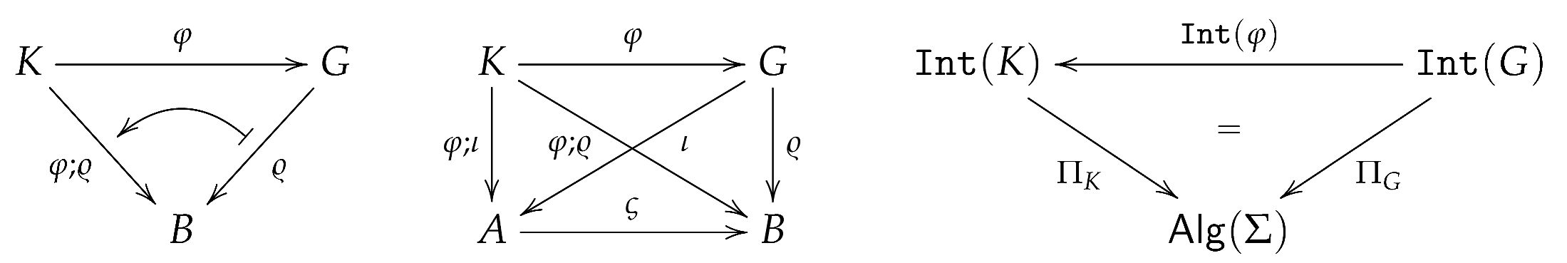
The assignments $K\mapsto \mathtt{Int}\left(K\right)$ and $\phi \mapsto \mathtt{Int}\left(\phi \right)$ define a functor $\mathtt{Int}:{\mathsf{Cxt}}_{EQ}^{op}\to \mathsf{Cat}$. This is the model functor of an Institution of Equations.

4.2. Terms and Equations

To define equations, we need terms! For any S-set K the S-set $T_{\Sigma }\left(K\right)$ of all $\Sigma$-terms on K is defined inductively as the smallest S-set such that:

• $K\subseteq T_{\Sigma }\left(K\right)$
• $\omega \langle \rangle \in T_{\Sigma }{\left(K\right)}_{out\left(\omega \right)}$ for all $\omega \in \Omega$ with $in\left(\omega \right)$ the empty S-set $\mathbf{0}=(\varnothing \mid s\in S)$.
• $\omega \langle {\tau }_{s_1}\left(x_1\right),\dots ,{\tau }_{s_n}\left(x_n\right)\rangle \in T_{\Sigma }{\left(K\right)}_{out\left(\omega \right)}$ for all $\omega \in \Omega$ with $in\left(\omega \right)$ non-empty and all S-maps $\tau :in\left(\omega \right)\to T_{\Sigma }\left(K\right)$ where $[x_1:s_1,x_2:s_2,\dots ,x_n:s_n]$ is the assumed representation of $in\left(\omega \right)$ as a list of variable declarations.

A $\Sigma$-equation $(K,t_1=t_2)$ in K is given by two $\Sigma$-terms $t_1,t_2\in T_{\Sigma }{\left(K\right)}_s$ for some $s\in S$ and $\mathtt{Eq}\left(K\right)$ denotes the set of all $\Sigma$-equations $(K,t_1=t_2)$ in K. In the usual way, the inductive definition of $\Sigma$-terms allows us to extend any S-map $\phi :K\to G$ between S-sets to an S-map ${\phi }^{*}:T_{\Sigma }\left(K\right)\to T_{\Sigma }\left(G\right)$ such that $\subseteq ;{\phi }^{*}=\phi ;\subseteq$ thus $\phi :K\to G$ induces a map $\mathtt{Eq}\left(\phi \right):\mathtt{Eq}\left(K\right)\to \mathtt{Eq}\left(G\right)$ with:

$$\mathtt{Eq}\left(\phi \right)(K,t_1=t_2):=(G,{\phi }^{*}\left(t_1\right)={\phi }^{*}\left(t_2\right))$$

(7)

for all $\Sigma$-equations $(K,t_1=t_2)$ in K.

Since $i{d}_K^{*}=i{d}_{T_{\Sigma }\left(K\right)}$ and ${(\phi ;\psi )}^{*}={\phi }^{*};{\psi }^{*}$ for all $\phi :K\to G$, $\psi :G\to H$, the assignments $K\mapsto \mathtt{Eq}\left(K\right)$ and $\phi \mapsto \mathtt{Eq}\left(\phi \right)$ define a functor $\mathtt{Eq}:{\mathsf{Cxt}}_{EQ}\to \mathsf{Set}$. This is the sentence functor of an Institution of Equations.

The semantics of terms is based on the evaluation of terms in algebras: Due to the inductive definition of $\Sigma$-terms, we can extend any interpretation $\iota :K\to A$ of a context K in a $\Sigma$-algebra $\mathcal{A}=(A,{\Omega }^{\mathcal{A}})$ to an S-map ${\iota }^{\circ }:T_{\Sigma }\left(K\right)\to A$ such that:

$$\subseteq ;{\iota }^{\circ }=\iota .$$

(8)

In such a way, we can define the semantics $t^{\mathcal{A}}$ of a $\Sigma$-term $t\in T_{\Sigma }\left(K\right),s\in S$ in a $\Sigma$-algebra $\mathcal{A}$ as a map $t^{\mathcal{A}}:A^K\to A_s$ defined by $t^{\mathcal{A}}\left(\iota \right):={\iota }^{\circ }\left(t\right)$ for all $\iota :K\to A$. Thus, feature expressions represent derived properties while terms represent derived operations!

4.3. Satisfaction Relation and Satisfaction Condition

Definition 15

(Satisfaction relation for equations).

For any context $K\in {\mathsf{Cxt}}_{EQ}$, any Σ-equation $(K,t_1=t_2)$ in K and any interpretation $(\iota ,\mathcal{A})$ of context K in a Σ-algebra $\mathcal{A}=(A,{\Omega }^{\mathcal{A}})$, we define:

$$(\iota ,\mathcal{A}){\vDash }_K(K,t_1=t_2)iff{\iota }^{\circ }\left(t_1\right)={\iota }^{\circ }\left(t_2\right)(i.e.t_1^{\mathcal{A}}\left(\iota \right)=t_2^{\mathcal{A}}\left(\iota \right))$$

(9)

The satisfaction condition is ensured by the well-behaved interplay of translations of terms along context morphisms and evaluations of terms.

Proposition 1

(Satisfaction condition for equations). For any morphism $\phi :K\to G$ in ${\mathsf{Cxt}}_{EQ}$, any Σ-equation $(K,t_1=t_2)$ in K and any interpretation $(\varrho ,\mathcal{A})$ of context G in a Σ-algebra $\mathcal{A}=(A,{\Omega }^{\mathcal{A}})$, we have:

$$\mathtt{Int}\left(\phi \right)(\varrho ,\mathcal{A}){\vDash }_K(K,t_1=t_2)iff(\varrho ,\mathcal{A}){\vDash }_G\mathtt{Eq}\left(\phi \right)(K,t_1=t_2).$$

(10)

Proof. 

Due to the definition of the functors $\mathtt{Int}:{\mathsf{Cxt}}_{EQ}^{op}\to \mathsf{Cat}$, $\mathtt{Eq}:{\mathsf{Cxt}}_{EQ}\to \mathsf{Set}$ and the fact that ${(\phi ;\varrho )}^{\circ }={\phi }^{*};{\varrho }^{\circ }$, we obtain the commutative diagram, above on the right, thus the satisfaction condition follows immediately from Definition 15. □

Summarizing all definitions and results, we obtain the main result in this section:

Proposition 2

(Institution of Equations). Any choice of a finite set S and a signature $\Sigma =(\Omega ,in,out)$ establishes a corresponding Institution of Equations $\mathcal{IE}=({\mathsf{Cxt}}_{EQ},\mathtt{Eq},\mathtt{Int},\vDash )$.

5. Sketches

Any institution gives us a corresponding category of presentations and an extension of the model functor of the institution to the category of presentations at hand [2,31]. We outline this construction for Institutions of Statements and Institutions of Equations.

We would like to use a specific term to distinguish presentations for Institutions of Statements or Equations, resp., from presentations in general. Since many of our motivating examples are variants of sketches, we will simply use the term sketch. In Section 5.1 and Section 5.2, we concentrate on sketches for Institutions of Statements while Section 5.3 outlines the corresponding variations for Institutions of Equations.

5.1. Sketches of Statements: Syntax and Semantics

To be prepared for the topics in Section 6, we introduce a very abstract and semantics-independent concept of sketch.

Definition 16

(Sketch). Let us have a category $\mathsf{Ct}$ of contexts and a functor $\mathtt{St}:\mathsf{Ct}\to \mathsf{Set}$, assigning to each $K\in {\mathsf{Ct}}_{Obj}$ a set $\mathtt{St}\left(K\right)$ of all statements in context K.

An$\mathtt{St}$- sketch$\mathbb{K}=(K,S{t}^{\mathbb{K}})$ is given by a context $K\in {\mathsf{Ct}}_{Obj}$ and a set $S{t}^{\mathbb{K}}\subseteq \mathtt{St}\left(K\right)$ of statements in context K.

In this subsection, we consider the case $\mathsf{Ct}=\mathsf{Cxt}$, $\mathtt{St}=\mathtt{Stm}$ with $\mathcal{IS}=(\mathsf{Cxt},\mathtt{Stm},\mathtt{Int},\vDash )$ an arbitrary Institution of Statements according to Theorem 1.

All definitions and constructions are, however, institution-independent; thus, they apply analogously to the case $\mathsf{Ct}={\mathsf{Cxt}}_{EQ}$, $\mathtt{St}=\mathtt{Eq}$ with $\mathcal{IE}=({\mathsf{Cxt}}_{EQ},\mathtt{Eq},\mathtt{Int},\vDash )$ an arbitrary Institution of Equations according to Proposition 2.

Example 36

(FOL: Sketches). We extend the sample context K in Example 31 to an ${\mathtt{Stm}}_{FOL}$-sketch $\mathbb{K}$ with the atomic statements (facts) $\mathtt{parent}(Anna,Uwe,Gabi)$, $\mathtt{parent}(Uwe,Heinz,Dora)$, $\mathtt{male}\left(Michael\right)$ and the proper first-order statements $\left(\right[y:prs],sbl,(y\mapsto Michael\left)\right)$, $\left(\right[y:prs],sbl,(y\mapsto Uwe\left)\right)$, $\left(\right[y:prs,x:nat],younger,(y\mapsto Michael,x\mapsto 12\left)\right)$, $\left(\right[y:prs],sbl,(y\mapsto Gabi\left)\right)$. The expression $[y:prs]▹sbl$, representing the property being sibling of someone, and the expression $[y:prs,x:nat]▹younger$, representing the property younger than, are defined in Example 26.

Example 37

(ALC: Sketches). Contexts in ALC are sets $N_O$ of individual names as already mentioned in Example 32. A concept assertion in ALC, i.e., a statement of the form $a:\mathtt{C}$ with $a\in N_O$ and $\mathtt{C}$ a (derived) concept, can be seen as a statement $(\left\{x_1\right\},\mathtt{C}\left(x_1\right),(x_1\mapsto a))$ in $N_O$ where the assignment $(x_1\mapsto a)$ defines a binding $\beta :\left\{x_1\right\}\to N_O$ with $\beta \left(x_1\right)=a$.

A role assertion, i.e., a statement of the form $(a,b):\mathtt{R}$ where $a,b\in N_O$ and $\mathtt{R}$ is a role, can be seen as a statement $(\{x_1,x_2\},\mathtt{R}(x_1,x_2),(x_1\mapsto a,x_2\mapsto b))$ in $N_O$. An ABox in ALC is a finite set of assertional axioms. Thus, a pair $(N_O,\mathcal{A})$ of a set $N_O$ of individual names and an ABox $\mathcal{A}$ of assertional axioms in $N_O$ is just an ${\mathtt{Stm}}_{ALC}$-sketch in our sense.

Example 38

(mFOL: Sketches). We extend the context $(K,{\tau }_K:K\to M_{mF})$ in Example 33 to an ${\mathtt{Stm}}_{mF}$-sketch with the atomic statements $\mathtt{un}(male:\mathit{P},prs:\mathit{S})$, $\mathtt{bin}(less:\mathit{P},nat:\mathit{S},nat:\mathit{S})$, $\mathtt{bin}(age:\mathit{P},prs:\mathit{S},nat:\mathit{S})$ and $\mathtt{trt}(parent:\mathit{P},prs:\mathit{S},prs:\mathit{S},prs:\mathit{S})$.

Obviously, this ${\mathtt{Stm}}_{mF}$-sketch describes exactly the sample footprint ${\Xi }_{FOL}$ in Example 11! Actually, we can describe all FOL-footprints, declaring only unary, binary or tertiary predicate symbols, as ${\mathtt{Stm}}_{mF}$-sketches. This fact confirms that the mFOL-example establishes indeed a meta-level for the FOL-example.

We have to be aware, however, that not all ${\mathtt{Stm}}_{mF}$-sketches correspond to FOL-footprints. For each predicate symbol in a FOL-footprint, we have to declare an arity, and this arity should be unique! Therefore, only those ${\mathtt{Stm}}_{mF}$-sketches, with exactly one atomic statement for each element in ${\tau }_K^{-1}\left(\mathit{P}\right)$ correspond to FOL-footprints. To describe those requirements concerning the structure of sketches, we can utilize sketch implications, introduced in the next subsection, and/or sketch constraints introduced in Section 6.

Example 39

(CT: Sketches). These are just the sketches, as we know them from Category Theory, with the essential difference that we are not restricting ourselves to commutative, limit and colimit statements only. We do not need to encode, for example, the concept monomorphism by means of pullbacks but can define it directly as a property of edges utilizing the ${\Xi }_{CT}$-expressions we discussed in Example 29.

As an example, we consider the context G from Example 34 and extend it to an ${\mathtt{Stm}}_{CT}$-sketch $\mathbb{G}=(G,S{t}^{\mathbb{G}})$ visualized above. $S{t}^{\mathbb{G}}$ contains the atomic statements $\mathtt{cmp}(a,b,e)$, $\mathtt{cmp}(a,b,f)$, $\mathtt{cmp}(c,d,g)$ and the proper first-order statements:

$(xv,fnl,(xv\mapsto 3\left)\right)$, $(x{v}_1\stackrel{xe}{\to }x{v}_2,mon,(xe\mapsto b))$, $(x{v}_1\stackrel{xe}{\to }x{v}_2,mon,(xe\mapsto g))$.

Example 40

(RM: Sketches). We extend the sample context $(K,{\tau }_K)$ from Example 35 to an ${\mathtt{Stm}}_{RM}$-sketch $\mathbb{K}=(K,S{t}^{\mathbb{K}})$. First, we declare two tables, i.e., $S{t}^{\mathbb{K}}$ contains two atomic statements $\mathtt{tb}\left(\mathtt{3}\right)\left({\gamma }_1\right)$, $\mathtt{tb}\left(\mathtt{3}\right)\left({\gamma }_2\right)$ with bindings ${\gamma }_1$ and ${\gamma }_2$ visualized by the following typed graphs:

Then, we declare for each table a primary key, i.e., we add two atomic statements $\mathtt{pk}\left({\gamma }_3\right)$, $\mathtt{pk}\left({\gamma }_4\right)$ with bindings ${\gamma }_3$, ${\gamma }_4$ given by $Empl:\mathit{T}\stackrel{eid:\mathbf{c}}{\to }Int:\mathit{D}$ and $Addr:\mathit{T}\stackrel{A.ssn:\mathbf{c}}{\to }Int:\mathit{D}$. Moreover, we declare a foreign key $\mathtt{fk}\left({\gamma }_5\right)$ with ${\gamma }_5$ depicted by $Empl:\mathit{T}\stackrel{E.ssn:\mathbf{c}}{\to }Int:\mathit{D}\stackrel{A.ssn:\mathbf{c}}{\leftarrow }x{t}_2:\mathit{T}$.

We could also require that each employee has a name and add an atomic statement $\mathtt{tot}\left({\gamma }_6\right)$ with ${\gamma }_6$ given by $Empl:\mathit{T}\stackrel{name:\mathbf{c}}{\to }String:\mathit{D}$.

Analogously to the requirements in Example 38, we do have the requirement that a table identifier can only appear once in a $\mathtt{tb}\left(\mathtt{n}\right)$-statement. There are, however, other database specific requirements: Any table should have exactly one primary key, a foreign key has to refer to a primary key, and others. As said before, to describe those kinds of structural requirements, we need sketch implications and/or sketch constraints. □

For any context K in $\mathsf{Cxt}$, any set $S\subseteq \mathtt{Stm}\left(K\right)$ of statements in K and any interpretation $(\iota ,\mathcal{U})$ of context K in a $\Xi$-structure $\mathcal{U}$ we define, relying on Definition 14:

$$(\iota ,\mathcal{U}){\vDash }_{K}Siff(\iota ,\mathcal{U}){\vDash }_K(X,Ex,\gamma )forall(X,Ex,\gamma )\in S.$$

(11)

Be aware that the statements in S may have different variable declarations X.

Definition 17

(Interpretation of sketch). A valid interpretation (model)of an $\mathtt{Stm}$-sketch $\mathbb{K}=(K,S{t}^{\mathbb{K}})$ is an interpretation $(\iota ,\mathcal{U})$ of context K such that $(\iota ,\mathcal{U}){\vDash }_{K}S{t}^{\mathbb{K}}$.

We denote by $\mathtt{Int}\left(\mathbb{K}\right)$ the full subcategory of $\mathtt{Int}\left(K\right)$ determined by all valid interpretations of $\mathbb{K}$ and by ${\Pi }_{\mathbb{K}}:\mathtt{Int}\left(\mathbb{K}\right)\to \mathsf{Sem}(\Xi )$ we denote the corresponding restriction of the projection functor ${\Pi }_K:\mathtt{Int}\left(K\right)\to \mathsf{Sem}(\Xi )$.

Remark 21

(Traditional presentations). If $\mathsf{Base}$ has an initial object $\mathbf{0}$, we can consider sketches $(\mathbf{0},S{t}^{})$ with $S{t}^{}$ only containing closed formulas, i.e., statements of the form $(\mathbf{0},Ex,i{d}_{\mathbf{0}})$ (see Remark 15). As discussed before, the projection functor ${\Pi }_{\mathbf{0}}:\mathtt{Int}\left(\mathbf{0}\right)\to \mathsf{Sem}(\Xi )$, due to Definition 13, is an isomorphism. In such a way, $(\mathbf{0},S{t}^{})$ is not only determining the interpretation subcategory $\mathtt{Int}(\mathbf{0},S{t}^{})⊑\mathtt{Int}\left(\mathbf{0}\right)$ but can also be seen as a presentation (specification) of the corresponding full subcategory $\mathsf{Sem}(\Xi ,(\mathbf{0},S{t}^{})):={\Pi }_{\mathbf{0}}\left(\mathtt{Int}(\mathbf{0},S{t}^{})\right)$ of $\mathsf{Sem}(\Xi )$ isomorphic to $\mathtt{Int}(\mathbf{0},S{t}^{})$.

In other words: due to Remark 18, we can describe $\mathsf{Sem}(\Xi ,(\mathbf{0},S{t}^{}))$ as the full subcategory of $\mathsf{Sem}(\Xi )$ given by all Ξ-structures $\mathcal{U}=(U,{\Phi }^{\mathcal{U}})$ in $\mathsf{Sem}(\Xi )$ such that $\mathcal{U}\vDash (\mathbf{0},Ex,i{d}_{\mathbf{0}})$ for all closed formulas $(\mathbf{0},Ex,i{d}_{\mathbf{0}})$ in $S{t}^{}$.

Example 41

(FOL: Interpretations). If we interpret the symbolic literals in $K_{prs}=\{Anna,Michael,Dora,Heinz,Sorin,Gabi,Uwe\}$ by the real persons in our family in December 2021, we will not obtain a valid interpretation of the ${\mathtt{Stm}}_{FOL}$-sketch $\mathbb{K}$ in Example 36 since the statement $\left(\right[y:prs],sbl,(y\mapsto Gabi\left)\right)$ is not satisfied by this interpretation. If we use, however, the statement $\left(\right[y:prs],\neg sbl,(y\mapsto Gabi\left)\right)$ instead, the interpretation becomes valid.

Note that the statement $\left(\right[y:prs],sbl,(y\mapsto Uwe\left)\right)$ is satisfied by the interpretation even if there is no witness for this statement in the context. $Uwe$’s only sister $Brita$ is not present in the context K!

Example 42

(mFOL: Interpretations). An interpretation of the sample context $(K,{\tau }_K)$ assigns to each element in ${\tau }_K^{-1}\left(\mathit{S}\right):=\{prs,nat\}$ and ${\tau }_K^{-1}\left(\mathit{P}\right):=\{\mathtt{parent},\mathtt{male},\mathtt{age},\mathtt{less}\}$, respectively, a set. Since ${\mathsf{Base}}_{mF}$ is the slice category $\mathsf{SET}/M_{mF}$, a certain set can either serve as a sort or as a predicate.

Our choice of $\mathsf{Sem}\left({\Xi }_{mF}\right)$ in Example 23 ensures, in addition, that the valid interpretations of the sample ${\mathtt{Stm}}_{mF}$-sketch from Example 38 are in one-to-one correspondence to the ${\Xi }_{FOL}$-structures in $\mathsf{Sem}\left({\Xi }_{FOL}\right)=\mathsf{Str}\left({\Xi }_{FOL}\right)$. We do have such a semantical one-to-one correspondence for any FOL-footprint, declaring only unary, binary or tertiary predicate symbols, and the corresponding ${\mathtt{Stm}}_{mF}$-sketch. This confirms that the mFOL-example establishes a meta-level for the FOL-example also w.r.t. semantics.

It is maybe worth mentioning that any ${\mathtt{Stm}}_{mF}$-sketch with two different atomic statements for, at least, one element in ${\tau }_K^{-1}\left(\mathit{P}\right)$ has no valid interpretation at all in $\mathsf{Sem}\left({\Xi }_{mF}\right)$.

Example 43

(Category Theory: Interpretations). Since we defined in Example 24 a very liberal semantics, we do have interpretations $(\iota ,\mathcal{U})$, $\mathcal{U}=(U,{\Phi }_{CT}^{\mathcal{U}})$ of the sample ${\mathtt{Stm}}_{CT}$-sketch $\mathbb{G}=(G,S{t}^{\mathbb{G}})$ in Example 39, where the graph homomorphism $\iota :G\to U$ maps the edges e and f to different edges in U even if both are declared as the composition of a and b.

If we would have also included into the sketch $\mathbb{G}$ the general statement $(\mathbf{0},guc,{!}_G)$ with the closed expression $\mathbf{0}▹guc$ expressing the property composititon is always unique (see Example 29), $(\iota ,\mathcal{U})$ could be only a valid interpretation of $\mathbb{G}$ if ι identifies e and f.

Example 44

(RM: Interpretations). Analogously to Example 42, our choice of $\mathsf{Sem}\left({\Xi }_{RM}\right)$ in Example 25 ensures that the valid interpretations of “well-formed” ${\mathtt{Stm}}_{RM}$-sketches, i.e., ${\mathtt{Stm}}_{RM}$-sketches representing database schemata, formalize exactly the traditional semantics of database schemata as outlined in Section 3.1.5.

Morphisms between sketches are defined by means of semantic entailment in a certain Institution of Statements $\mathcal{IS}=(\mathsf{Cxt},\mathtt{Stm},\mathtt{Int},\vDash )$.

Definition 18

(Statement entailment). For any context K in $\mathsf{Cxt}$ and any sets $S,T\subseteq \mathtt{Stm}\left(K\right)$ of statements in K, we say that S entails T in a $\Xi$- structure $\mathcal{U}$, $S{⊩}_K^{\mathcal{U}}T$ in symbols, if, and only if, for all interpretations $(\iota ,\mathcal{U})$ of K in $\mathcal{U}$: $(\iota ,\mathcal{U}){\vDash }_{K}S$ implies $(\iota ,\mathcal{U}){\vDash }_{K}T$.

Sentails T, $S{⊩}_{K}T$ in symbols, if, and only if, $S{⊩}_K^{\mathcal{U}}T$ for all Ξ-structures $\mathcal{U}$ in $\mathsf{Sem}(\Xi )$.

Definition 19

(Sketch morphism). An $\mathcal{IS}$-morphism $\phi :\mathbb{K}⤏\mathbb{G}$ between two $\mathtt{Stm}$-sketches $\mathbb{K}=(K,S{t}^{\mathbb{K}})$, $\mathbb{G}=(G,S{t}^{\mathbb{G}})$ is a morphism $\phi :K\to G$ in $\mathsf{Cxt}$ such that $S{t}^{\mathbb{G}}{⊩}_G\mathtt{Stm}\left(\phi \right)\left(S{t}^{\mathbb{K}}\right)$. An $\mathcal{IS}$-morphism $\phi :\mathbb{K}⤏\mathbb{G}$ is calledstrictif $S{t}^{\mathbb{G}}\supseteq \mathtt{Stm}\left(\phi \right)\left(S{t}^{\mathbb{K}}\right)$.

$\mathsf{Sk}{\left(\mathcal{IS}\right)}^m$ denotes the category of all $\mathtt{Stm}$-sketches and all $\mathcal{IS}$-morphisms between them. Its subcategory of all $\mathtt{Stm}$-sketches and all strict $\mathcal{IS}$-morphisms is denoted by $\mathsf{Sk}{\left(\mathcal{IS}\right)}_s^m$.

We will consider three different kinds of directed relationships between sketches distinguished by three different kinds of arrow-symbols. We choose the arrow-symbol “⤏” for sketch morphisms since it is the kind of directed relationship we will mention the least.

If $\mathcal{IS}$ is clear from the context, we will also use the shorthand notations ${\mathsf{Sk}}^m$ and ${\mathsf{Sk}}_s^m$ instead of $\mathsf{Sk}{\left(\mathcal{IS}\right)}^m$ and $\mathsf{Sk}{\left(\mathcal{IS}\right)}_s^m$, respectively.

$\mathcal{IS}$-morphisms $\phi :\mathbb{K}⤏\mathbb{G}$ with $K=G$ and $\phi =i{d}_K$ simply reflect statement entailments. For any $\mathcal{IS}$-morphism $\phi :\mathbb{K}⤏\mathbb{G}$, the condition $S{t}^{\mathbb{G}}{⊩}_G\mathtt{Stm}\left(\phi \right)\left(S{t}^{\mathbb{K}}\right)$ ensures, due to the satisfaction condition that the functor $\mathtt{Int}\left(\phi \right):\mathtt{Int}\left(G\right)\to \mathtt{Int}\left(K\right)$ restricts to a functor from $\mathtt{Int}$($\mathbb{G}$) into $\mathtt{Int}$($\mathbb{K}$). In such a way, the assignments $\mathbb{K}\mapsto \mathtt{Int}\left(\mathbb{K}\right)$ extend to a functor ${\mathtt{Int}}^{\mathsf{Sk}}:{\left({\mathsf{Sk}}^m\right)}^{op}\to \mathsf{Cat}$.

According to well-known general results (see Corollary 4.3 in [2]), we know that ${\mathsf{Sk}}^m$ has whatever limits or colimits the category $\mathsf{Cxt}$ has since limits and colimits in the category ${\mathsf{Sk}}^m$ of $\mathtt{Stm}$-sketches and $\mathcal{IS}$-morphisms are constructed by means of limits and colimits in the category $\mathsf{Cxt}$, respectively (compare Propositions 5 and 6). This ensures also that we do have amalgamation [1,2,38]: ${\mathtt{Int}}^{\mathsf{Sk}}:{\left({\mathsf{Sk}}^m\right)}^{op}\to \mathsf{Cat}$ maps all colimits in $\mathsf{Cxt}$ that are preserved by the inclusion $\mathsf{Cxt}⊑\mathsf{Base}$, to limits in $\mathsf{Cat}$.

The Theory of Institutions gives us “for free” $\mathtt{Stm}$-sketches, $\mathcal{IS}$-morphisms, the category ${\mathsf{Sk}}^m$ as well as the extended model functor${\mathtt{Int}}^{\mathsf{Sk}}:{\left({\mathsf{Sk}}^m\right)}^{op}\to \mathsf{Cat}$.

However, to employ sketches as a specification formalism and to develop deduction calculi for sketches, we need a number of other concepts, constructions and results.

5.2. Sketches of Statements vs. Structures

In the Introduction, we discussed, among other things, two central motivations for the development of our framework: (1) We want to be able to give a general abstract account of the concept of free structures generalizing concepts like a group generated by a set of generators and a set of defining relations. (2) We want to provide an alternative general mechanism to encode structures “syntactically” that avoids the kind of circularity inherent to the technique of “signature extensions”.

In the remaining part of this section, we outline proposals to meet these objectives.

5.2.1. Freely Generated Structures

To reconstruct the concept of a group generated by a set of generators and a set of defining relations, we need operations only. Those cases of free algebras are discussed in Section 5.3.1.

First, We Consider Structures Freely Generated in $\mathsf{Sem}(\Xi )$

A $\Xi$-structure $\mathcal{F}=(F,{\Phi }^{\mathcal{F}})$ is freely generated in $\mathsf{Sem}(\Xi )$ by an $\mathtt{Stm}$-sketch $\mathbb{G}=(G,S{t}^{\mathbb{G}})$ if, and only if, $\mathcal{F}$ is in $\mathsf{Sem}(\Xi )$ and there is a valid interpretation$({\eta }_{\mathbb{G}},\mathcal{F})$ of $\mathbb{G}$ in $\mathcal{F}$ that is universal relative to $\mathsf{Sem}(\Xi )$. That is, for all $\Xi$-structures $\mathcal{U}=(U,{\Phi }^{\mathcal{U}})$ in $\mathsf{Sem}(\Xi )$ and all valid interpretations $(\iota ,\mathcal{U})$ of $\mathbb{G}$ in $\mathcal{U}$ there exists a unique morphism ${\iota }^{*}:\mathcal{F}\to \mathcal{U}$ in $\mathsf{Sem}(\Xi )$ such that ${\eta }_{\mathbb{G}};{\iota }^{*}=\iota$ in $\mathsf{Base}$, i.e., such that ${\iota }^{*}$ establishes an interpretation morphism ${\iota }^{*}:({\eta }_{\mathbb{G}},\mathcal{F})\to (\iota ,\mathcal{U})$ in $\mathtt{Int}\left(\mathbb{G}\right)⊑\mathtt{Int}\left(G\right)$ according to Definition 13.

A $\Xi$-structure, freely generated in $\mathsf{Sem}(\Xi )$ by an $\mathtt{Stm}$-sketch $\mathbb{G}=(G,S{t}^{\mathbb{G}})$, is obviously uniquely determined “up to isomorphism in $\mathsf{Sem}(\Xi )$” if it exists.

The universal property of $({\eta }_{\mathbb{G}},\mathcal{F})$ entails that $({\eta }_{\mathbb{G}},\mathcal{F})$ is initial in $\mathtt{Int}$($\mathbb{G}$), thus the projection functor ${\Pi }_{\mathbb{G}}:\mathtt{Int}\left(\mathbb{G}\right)\to \mathsf{Sem}(\Xi )$ establishes a functor from $\mathtt{Int}$($\mathbb{G}$) into the co-slice category $\mathcal{F}/\mathsf{Sem}(\Xi )$.

In the case that $S{t}^{\mathbb{G}}$ contains only atomic statements, the definition of morphisms between $\Xi$-structures ensures $({\eta }_{\mathbb{G}};\varrho ,\mathcal{U}){\vDash }_{G}S{t}^{\mathbb{G}}$ for any morphism $\varrho :\mathcal{F}\to \mathcal{U}$ in $\mathsf{Sem}(\Xi )$; thus, the assignments $(\varrho :\mathcal{F}\to \mathcal{U})\mapsto ({\eta }_{\mathbb{G}};\varrho ,\mathcal{U})$ establish a functor from $\mathcal{F}/\mathsf{Sem}(\Xi )$ into $\mathtt{Int}\left(\mathbb{G}\right)$. Due to the universal property of $({\eta }_{\mathbb{G}},\mathcal{F})$, we obtain ${({\eta }_{\mathbb{G}};\varrho )}^{*}=\varrho$. Together with the equation ${\eta }_{\mathbb{G}};{\iota }^{*}=\iota$, this ensures that the two functors establish an isomorphism between $\mathtt{Int}\left(\mathbb{G}\right)$ and $\mathcal{F}/\mathsf{Sem}(\Xi )$ (compare Proposition 4.10 in [2]). This justifies that we can call, in this atomic case, the pair $(\mathbb{G},{\eta }_{\mathbb{G}})$ a sketch representation of $\mathcal{F}$.

Note that the $\Xi$-structure $(G,{\Phi }^{\varnothing })$ with ${\Phi }^{\varnothing }$ a $\Phi$-indexed family of empty sets is trivially freely generated in $\mathsf{Sem}(\Xi )$ by $\mathbb{G}=(G,\varnothing )$.

Second, We Consider Structures Freely Generated Relative to a Subcategory $\mathsf{D}$:

Let $\mathsf{D}$ be an arbitrary full subcategory of $\mathsf{Sem}(\Xi )$. A $\Xi$-structure $\mathcal{F}=(F,{\Phi }^{\mathcal{F}})$ is freely generated in $\mathsf{D}$ by an $\mathtt{Stm}$-sketch $\mathbb{G}=(G,S{t}^{\mathbb{G}})$ if, and only if, $\mathcal{F}$ is an object in $\mathsf{D}$ and there is a valid interpretation $({\eta }_{\mathbb{G}},\mathcal{F})$ of $\mathbb{G}$ in $\mathcal{F}$ that is universal relative to $\mathsf{D}$. That is, for all $\Xi$-structures $\mathcal{U}=(U,{\Phi }^{\mathcal{U}})$ in $\mathsf{D}$ and all valid interpretations $(\iota ,\mathcal{U})$ of $\mathbb{G}$ in $\mathcal{U}$ there exists a unique morphism ${\iota }^{*}:\mathcal{F}\to \mathcal{U}$ in $\mathsf{D}$ such that ${\eta }_{\mathbb{G}};{\iota }^{*}=\iota$ in $\mathsf{Base}$, i.e., such that ${\iota }^{*}$ establishes an interpretation morphism ${\iota }^{*}:({\eta }_{\mathbb{G}},\mathcal{F})\to (\iota ,\mathcal{U})$ in $\mathtt{Int}\left(\mathbb{G}\right)⊑\mathtt{Int}\left(G\right)$.

A $\Xi$-structure, freely generated in $\mathsf{D}$ by an $\mathtt{Stm}$-sketch $\mathbb{G}=(G,S{t}^{\mathbb{G}})$ is, obviously, uniquely determined “up to isomorphism in $\mathsf{D}$” if it exists. In this case, the universal property of $({\eta }_{\mathbb{G}},\mathcal{F})$ entails that $({\eta }_{\mathbb{G}},\mathcal{F})$ is initial in the subcategory $\mathtt{Int}\left(\mathbb{G}\right)\downarrow \mathsf{D}:={\Pi }_G^{-1}\left(\mathsf{D}\right)$ of all valid interpretations of $\mathbb{G}$ in $\Xi$-structures in $\mathsf{D}$. Analogous to the case $\mathsf{D}=\mathsf{Sem}(\Xi )$, we obtain, moreover, an isomorphism between $\mathtt{Int}\left(\mathbb{G}\right)\downarrow \mathsf{D}$ and the co-slice category $\mathcal{F}/\mathsf{D}$ if $S{t}^{\mathbb{G}}$ contains only atomic statements.

Third, We Consider Subcategories Described by Logical Means

One logical means to describe subcategories of $\mathsf{Sem}(\Xi )$ are $\mathtt{Stm}$-sketches $(\mathbf{0},S{t}^{})$ with $S{t}^{}$ only containing closed formulas, i.e., statements of the form $(\mathbf{0},Ex,i{d}_{\mathbf{0}})$. As discussed in Remark 21, those sketches can be seen as presentations in the traditional sense of the Theory of Institutions specifying subcategories $\mathsf{Sem}(\Xi ,(\mathbf{0},S{t}^{}))$ of $\mathsf{Sem}(\Xi )$.

As another logical means to describe subcategories of $\mathsf{Sem}(\Xi )$, we will introduce sketch implications in Section 5.2.3 (see Remark 27).

5.2.2. Elementary Diagrams

To establish sketch-based mechanisms to encode structures “syntactically”, we have to assume an Institution of Statements $\mathcal{IS}=(\mathsf{Cxt},\mathtt{Stm},\mathtt{Int},\vDash )$ with $\mathsf{Carr}⊑\mathsf{Cxt}$ and $\mathtt{At}\left(K\right)\subseteq \mathtt{Stm}\left(K\right)$ for all contexts K in $\mathsf{Cxt}$, i.e., $\mathtt{Stm}\left(K\right)$ contains all atomic statements in K.

There are two canonical ways to transform a $\Xi$-structure $\mathcal{U}=(U,{\Phi }^{\mathcal{U}})$ into an $\mathtt{Stm}$-sketch. The atomic variant ${\mathbb{S}}_{\Phi }^{\mathcal{U}}=(U,S{t}_{\Phi }^{\mathcal{U}})$ encodes only the semantics of feature symbols and uses therefore only atomic statements:

$$S{t}_{\Phi }^{\mathcal{U}}:=\{(\alpha F,F\left(i{d}_{\alpha F}\right),\gamma )\mid F\in \Phi ,\gamma \in {\left[\left[F\right]\right]}^{\mathcal{U}}\}\subseteq \mathtt{At}\left(U\right).$$

(12)

The full variant ${\mathbb{S}}^{\mathcal{U}}=(U,S{t}^{\mathcal{U}})$ is available if $\mathtt{XE}(\Xi ,X)=\mathtt{FE}(\Xi ,X)$ for all $X\in {\mathsf{Var}}_{Obj}$ and encodes the semantics of all feature expressions:

$$S{t}^{\mathcal{U}}:=\{(X,Ex,\gamma )\mid X\in {\mathsf{Var}}_{Obj},Ex\in \mathtt{FE}(\Xi ,X),\gamma \in {\left[\left[Ex\right]\right]}_X^{\mathcal{U}}\}\subseteq \mathtt{Stm}\left(U\right).$$

(13)

We obviously have $S{t}_{\Phi }^{\mathcal{U}}\subset S{t}^{\mathcal{U}}$. For any statement $(X,Ex,\gamma )$ in U we obtain, according to (13) and the definition of satisfaction relations in Definition 14,

$$(X,Ex,\gamma )\in S{t}^{\mathcal{U}}iff\gamma ;i{d}_U=\gamma \in {\left[\left[Ex\right]\right]}_X^{\mathcal{U}}iff(i{d}_U,\mathcal{U}){\vDash }_U(X,Ex,\gamma ).$$

(14)

thus $(i{d}_U,\mathcal{U})$ is a valid interpretation of ${\mathbb{S}}_{\Phi }^{\mathcal{U}}$ as well as of ${\mathbb{S}}^{\mathcal{U}}$.

In traditional First-Order Logic, we meet the full variant in the form of elementary diagrams [39]. The difference to our encoding is that the carrier of a first-order structure is not considered as a context. Instead, each element of the carrier is added as a constant to the signature. The encoding of structures as sketches avoids this kind of circularity. The “signature extension trick” works only for first-order signatures with constants symbols and, more critically, it requires that the carriers of first-order structures are sets! It looks like the sketch encoding mechanism is much more flexible and general.

The elementary diagrams in [2] give an abstract account of the signature extension approach but are based on an atomic variant of encoding.

There are no structures at all in [15] only atomic sketches! In [13], we followed Makkai and have not considered structures either. Instead, we worked, directly, with the atomic sketch encodings ${\mathbb{S}}_{\Phi }^{\mathcal{U}}$ of structures.

To validate, in retrospective, the approaches in [13,15], a noticeable portion of the remaining part of the paper, will be spent to answer the following question:

Question 4: Is there any justification to ignore completely the concept of semantic structure (model)?

By construction, any $\Xi$-structure $\mathcal{U}=(U,{\Phi }^{\mathcal{U}})$ in $\mathsf{Sem}(\Xi )$ is freely generated in $\mathsf{Sem}(\Xi )$ by the $\mathtt{Stm}$-sketch ${\mathbb{S}}_{\Phi }^{\mathcal{U}}=(U,S{t}_{\Phi }^{\mathcal{U}})$ with the universal interpretation $(i{d}_U,\mathcal{U})$. $S{t}_{\Phi }^{\mathcal{U}}$ contains only atomic statements thus $({\mathbb{S}}_{\Phi }^{\mathcal{U}},i{d}_U)$ becomes a sketch representation of $\mathcal{U}$ in the sense of the last subsection. In particular, there is an isomorphism between $\mathtt{Int}\left({\mathbb{S}}_{\Phi }^{\mathcal{U}}\right)$ and $\mathcal{U}/\mathsf{Sem}(\Xi )$.

The crucial observation is, however, that the assignments $\mathcal{U}\mapsto {\mathbb{S}}_{\Phi }^{\mathcal{U}}$ define an embedding $\mathtt{Enc}:\mathsf{Str}(\Xi )\to \mathsf{Sk}{\left(\mathtt{Stm}\right)}^a$ of $\mathsf{Str}(\Xi )$ into the category $\mathsf{Sk}{\left(\mathtt{Stm}\right)}^a$ of all $\mathtt{Stm}$-sketches and all $\mathtt{Stm}$-sketch arrows defined in the next subsection in Definition 20. This embedding establishes, moreover, an isomorphism between $\mathsf{Str}(\Xi )$ and the subcategory $\mathsf{atSk}{\left(\mathtt{Stm}\right)}_s^a$ of $\mathsf{Sk}{\left(\mathtt{Stm}\right)}^a$ given by all atomic $\mathtt{Stm}$-sketches and all strict $\mathtt{Stm}$-sketch arrows between them. An $\mathtt{Stm}$-sketch $\mathbb{K}=(K,S{t}^{\mathbb{K}})$ is atomic if $S{t}^{\mathbb{K}}\subseteq \mathtt{At}\left(K\right)$ (see Remark 14).

The concepts (atomic) $\mathtt{Stm}$-sketch and (strict) $\mathtt{Stm}$-sketch arrow concern only the “structure” of sketches and are completely semantics-independent. That is, the transition along the encoding functor $\mathtt{Enc}$ from the category $\mathsf{Str}(\Xi )$ to the isomorphic category $\mathsf{atSk}{\left(\mathtt{Stm}\right)}_s^a$ implements an abstraction from the concept semantic structure (model) to the concept atomic sketch. In case $\mathsf{Sem}(\Xi )=\mathsf{Str}(\Xi )$, this abstraction is exhaustive. In case $\mathsf{Sem}{(\Xi )}_{Obj}⊊\mathsf{Str}{(\Xi )}_{Obj}$, however, we need an additional semantics-independent, purely structural characterization identifying exactly all those atomic $\mathtt{Stm}$-sketches ${\mathbb{S}}_{\Phi }^{\mathcal{U}}$ in $\mathsf{atSk}{\left(\mathtt{Stm}\right)}_s^a$ with $\mathcal{U}$ in $\mathsf{Sem}(\Xi )$, to make the abstraction complete (see Remark 29).

A sketch is constituted by a context and a set of statements. The informal term “structure of a sketch” takes into account the context; for each statement, the syntactic structure of the corresponding expression and its “location”, i.e., its binding morphism, the set of statements as such and the “distribution” of the statements over the context.

5.2.3. Sketch Arrows and Sketch Implications

We can not only transform $\Xi$-structures $\mathcal{U}$ into the $\mathtt{Stm}$-sketches ${\mathbb{S}}_{\Phi }^{\mathcal{U}}$ and ${\mathbb{S}}^{\mathcal{U}}$. We can even encode the validity of certain classes of “closed formulas” in $\mathcal{U}$ by means of semantics-independent, pure structural closedness properties of ${\mathbb{S}}_{\Phi }^{\mathcal{U}}$ or ${\mathbb{S}}^{\mathcal{U}}$, respectively. To see this, we need some preparations.

First, we have to take a step back and consider a very simple, semantics-independent relationship between sketches. To be prepared for Section 6, we define this relationship on the same level of abstraction as Definition 16 (Sketch).

Definition 20

(Sketch Arrow). Let us be given a category $\mathsf{Ct}$ and a functor $\mathtt{St}:\mathsf{Ct}\to \mathsf{Set}$. An arrow$\phi :\mathbb{K}\to \mathbb{G}$ between two $\mathtt{St}$-sketches $\mathbb{K}=(K,S{t}^{\mathbb{K}})$, $\mathbb{G}=(G,S{t}^{\mathbb{G}})$ is given by a context morphism $\phi :K\to G$. $\phi :\mathbb{K}\to \mathbb{G}$ is calledstrictif $S{t}^{\mathbb{G}}\supseteq \mathtt{St}\left(\phi \right)\left(S{t}^{\mathbb{K}}\right)$.

$\mathsf{Sk}{\left(\mathtt{St}\right)}^a$ denotes the category of all $\mathtt{St}$-sketches and all $\mathtt{St}$-sketch arrows between them. Its subcategory of all $\mathtt{St}$-sketches and all strict $\mathtt{St}$-sketch arrows is denoted by $\mathsf{Sk}{\left(\mathtt{St}\right)}_s^a$.

If $\mathtt{St}$ is clear from the context, we will also use the shorthand notations ${\mathsf{Sk}}^a$ and ${\mathsf{Sk}}_s^a$ instead of $\mathsf{Sk}{\left(\mathtt{St}\right)}^a$ and $\mathsf{Sk}{\left(\mathtt{St}\right)}_s^a$, respectively. If $K=G$ and $\phi =i{d}_K$, we will also just write $\mathbb{K}\to \mathbb{G}$ instead of $\phi :\mathbb{K}\to \mathbb{G}$. We consider the case $\mathsf{Ct}=\mathsf{Cxt}$, $\mathtt{St}=\mathtt{Stm}$ with $\mathcal{IS}=(\mathsf{Cxt},\mathtt{Stm},\mathtt{Int},\vDash )$ an Institution of Statements.

Remark 22

(Sketch Morphisms vs. Sketch Arrows). An $\mathcal{IS}$-morphism $\phi :\mathbb{K}⤏\mathbb{G}$ is a $\mathtt{Stm}$-sketch arrow $\phi :\mathbb{K}\to \mathbb{G}$ satisfying the semantical morphism condition $S{t}^{\mathbb{G}}{⊩}_G\mathtt{Stm}\left(\phi \right)\left(S{t}^{\mathbb{K}}\right)$. Not every $\mathtt{Stm}$-sketch arrow $\phi :\mathbb{K}\to \mathbb{G}$ provides an $\mathcal{IS}$-morphism $\phi :\mathbb{K}⤏\mathbb{G}$, but each $\mathcal{IS}$-morphism $\phi :\mathbb{K}⤏\mathbb{G}$ has an underlying $\mathtt{Stm}$-sketch arrow$\phi :\mathbb{K}\to \mathbb{G}$.

Any strict $\mathtt{Stm}$-sketch arrow $\phi :\mathbb{K}\to \mathbb{G}$ satisfies, trivially, the morphism condition and provides, in such a way, a strict $\mathcal{IS}$-morphism $\phi :\mathbb{K}⤏\mathbb{G}$ due to Definition 19.

There is, however, another semantical condition that is kind of dual to the morphism condition. We call this condition the implication condition and, as a “terminological sleight of hand”, we introduce the concept of a “sketch implication”, simply indicating that a sketch arrow is intended to be the subject of this dual semantical condition.

Definition 21

(Sketch implication). An $\mathcal{IS}$- implication $\mathbb{P}\stackrel{\phi }{\Rightarrow }\mathbb{C}$ is given by two $\mathtt{Stm}$-sketches $\mathbb{P}=(P,S{t}^{\mathbb{P}})$, $\mathbb{C}=(C,S{t}^{\mathbb{C}})$ and a context morphism $\phi :P\to C$.

An $\mathcal{IS}$-implication $\mathbb{P}\stackrel{\phi }{\Rightarrow }\mathbb{C}$ is calledstrictif $S{t}^{\mathbb{C}}\supseteq \mathtt{Stm}\left(\phi \right)\left(S{t}^{\mathbb{P}}\right)$.

$\mathsf{Sk}{\left(\mathcal{IS}\right)}^i$ denotes the category of all $\mathtt{Stm}$-sketches and all $\mathcal{IS}$-implications between them. Its subcategory of all $\mathtt{Stm}$-sketches and all strict $\mathcal{IS}$-implications is denoted by $\mathsf{Sk}{\left(\mathcal{IS}\right)}_s^i$.

If $\mathcal{IS}$ is clear from the context, we will also use the shorthand notations ${\mathsf{Sk}}^i$ and ${\mathsf{Sk}}_s^i$ instead of $\mathsf{Sk}{\left(\mathcal{IS}\right)}^i$ and $\mathsf{Sk}{\left(\mathcal{IS}\right)}_s^i$, respectively. If $P=C$ and $\phi =i{d}_P$, we will also simply write $\mathbb{P}\Rightarrow \mathbb{C}$ instead of $\mathbb{P}\stackrel{i{d}_P}{⟹}\mathbb{C}$.

What we call the implication condition is nothing but the usual condition that an implication is valid if each “solution” of the premise gives rise to a “solution” of the conclusion.

Definition 22

(Validity of Sketch Implications). Let us be given an $\mathcal{IS}$-implication $\mathbb{P}\stackrel{\phi }{\Rightarrow }\mathbb{C}$ between two $\mathtt{Stm}$-sketches $\mathbb{P}=(P,S{t}^{\mathbb{P}})$ and $\mathbb{C}=(C,S{t}^{\mathbb{C}})$.

Aninterpretation $(\iota ,\mathcal{U})$of context P in a Ξ-structure $\mathcal{U}$satisfies$\mathbb{P}\stackrel{\phi }{\Rightarrow }\mathbb{C}$, $(\iota ,\mathcal{U})\vDash \mathbb{P}\stackrel{\phi }{\Rightarrow }\mathbb{C}$ in symbols, if, and only if, $(\iota ,\mathcal{U}){\vDash }_{P}S{t}^{\mathbb{P}}$ implies that there exists an interpretation $(\varrho ,\mathcal{U})$ of context C in $\mathcal{U}$ with $\phi ;\varrho =\iota$ such that $(\varrho ,\mathcal{U}){\vDash }_{C}S{t}^{\mathbb{C}}$.

$\mathbb{P}\stackrel{\phi }{\Rightarrow }\mathbb{C}$ is valid in a $\Xi$-structure $\mathcal{U}$, $\mathcal{U}\vDash \mathbb{P}\stackrel{\phi }{\Rightarrow }\mathbb{C}$ in symbols, if, and only if, we have $(\iota ,\mathcal{U})\vDash \mathbb{P}\stackrel{\phi }{\Rightarrow }\mathbb{C}$ for all interpretations $(\iota ,\mathcal{U})$ of P in $\mathcal{U}$.

$\mathbb{P}\stackrel{\phi }{\Rightarrow }\mathbb{C}$ isvalid (in $\mathcal{IS}$), $\vDash \mathbb{P}\stackrel{\phi }{\Rightarrow }\mathbb{C}$ in symbols, if, and only if, $\mathcal{U}\vDash \mathbb{P}\stackrel{\phi }{\Rightarrow }\mathbb{C}$ for all Ξ-structures $\mathcal{U}$ in $\mathsf{Sem}(\Xi )$.

Remark 23

(Subcategories of valid Sketch Implications). For any Ξ-structure $\mathcal{U}$ and any $\mathtt{Stm}$-sketch $\mathbb{P}$ we have $\mathcal{U}\vDash \mathbb{P}\stackrel{i{d}_P}{\Rightarrow }\mathbb{P}$. Moreover, $\mathcal{U}\vDash \mathbb{A}\stackrel{\phi }{\Rightarrow }\mathbb{B}$ and $\mathcal{U}\vDash \mathbb{B}\stackrel{\psi }{\Rightarrow }\mathbb{C}$ implies $\mathcal{U}\vDash \mathbb{A}\stackrel{\phi ;\psi }{⟹}\mathbb{C}$. In such a way, the collection of all $\mathcal{IS}$-implications, valid in a Ξ-structure $\mathcal{U}$, defines a corresponding subcategory of ${\mathsf{Sk}}^i$ with the same objects as ${\mathsf{Sk}}^i$.

Intersecting all those subcategories for all Ξ-structures $\mathcal{U}$ in $\mathsf{Sem}(\Xi )$, we obtain the subcategory ${\mathsf{Sk}}^i\left(\mathsf{Sem}(\Xi )\right)$ of ${\mathsf{Sk}}^i$ given by all $\mathcal{IS}$-implications valid in $\mathcal{IS}$.

Remark 24

(Sketch Implications vs. Sketch Arrows). An $\mathcal{IS}$-implication $\mathbb{P}\stackrel{\phi }{\Rightarrow }\mathbb{C}$ is simply another notation for a $\mathtt{Stm}$-sketch arrow $\phi :\mathbb{P}\to \mathbb{C}$. The only difference is that we allow $\mathbb{P}\stackrel{\phi }{\Rightarrow }\mathbb{C}$ to be the subject of semantical implication conditions , like $\mathcal{U}\vDash \mathbb{P}\stackrel{\phi }{\Rightarrow }\mathbb{C}$, while the corresponding $\mathtt{Stm}$-sketch arrow $\phi :\mathbb{P}\to \mathbb{C}$ is considered as a pure structural entity without any semantical significance.

In contrast to $\mathcal{IS}$-morphisms (compare Remark 22), a strict $\mathtt{Stm}$-sketch arrow $\phi :\mathbb{P}\to \mathbb{C}$ does not give, trivially, rise to an $\mathcal{IS}$-implication $\mathbb{P}\stackrel{\phi }{\Rightarrow }\mathbb{C}$ satisfying semantical implication conditions.

For any $\mathtt{Stm}$-sketch arrow $\phi :\mathbb{P}\to \mathbb{C}$, we can construct a respective strict $\mathtt{Stm}$-sketch arrow $\phi :\mathbb{P}\to {\mathbb{C}}^{\phi }$ with ${\mathbb{C}}^{\phi }:=(C,S{t}^{\mathbb{C}}\cup \mathtt{Stm}\left(\phi \right)\left(S{t}^{\mathbb{P}}\right))$. The satisfaction condition ensures that the corresponding $\mathcal{IS}$-implications $\mathbb{P}\stackrel{\phi }{\Rightarrow }\mathbb{C}$ and $\mathbb{P}\stackrel{\phi }{\Rightarrow }{\mathbb{C}}^{\phi }$ are semantically equivalent: $\mathcal{U}\vDash \mathbb{P}\stackrel{\phi }{\Rightarrow }\mathbb{C}$ if, and only if, $\mathcal{U}\vDash \mathbb{P}\stackrel{\phi }{\Rightarrow }{\mathbb{C}}^{\phi }$ for all Ξ-structures $\mathcal{U}$.

Remark 25

(Sketch Implications vs. Sketch Morphisms). The concepts sketch morphism and sketch implication are skewed but kind of dual. Sketch morphisms talk about “reducts of models” while sketch implications state the existence of “model extensions”.

In case $P=C$ and $\phi =i{d}_P$, a $\mathtt{Stm}$-sketch arrow $\phi :\mathbb{P}\to \mathbb{C}$ provides an $\mathcal{IS}$-morphism $i{d}_P:\mathbb{P}⤏\mathbb{C}$ if, and only if, $S{t}^{\mathbb{C}}{⊩}_{P}S{t}^{\mathbb{P}}$ while the validity in $\mathcal{IS}$ of the corresponding $\mathcal{IS}$-implication $\mathbb{P}\stackrel{}{\Rightarrow }\mathbb{C}$ means semantic entailment exactly in the opposite direction $S{t}^{\mathbb{P}}{⊩}_{P}S{t}^{\mathbb{C}}$!

Remark 26

(Deduction Rules). Attention, the exposition in the following remarks and examples, relies implicitly on the observation that sketch arrows can be utilized asdeduction rules. A deduction rule, given by a $\mathtt{Stm}$-sketch arrow $\phi :\mathbb{P}\to \mathbb{C}$, issoundfor a certain Institution of Statements $\mathcal{IS}=(\mathsf{Cxt},\mathtt{Stm},\mathtt{Int},\vDash )$ if, and only if, the respective $\mathcal{IS}$-implication $\mathbb{P}\stackrel{\phi }{\Rightarrow }\mathbb{C}$ is valid in $\mathcal{IS}$!

The utilization of sketch arrows as deduction rules is triggered by Definition 23 as well as Proposition 3 and Corollary 2 at the end of this subsection and will be discussed shortly in Remark 32.

Remark 27

(Valid Sketch Implications and Axioms). There are $\mathcal{IS}$-implications (or, more precisely, $\mathcal{IS}$-implication schemata) that areuniversalin the sense that they are valid in any Institution of Statements $\mathcal{IS}=(\mathsf{Cxt},\mathtt{Stm},\mathtt{Int},\vDash )$, since they reflect the structure and semantics of feature expressions. In particular, the introduction and elimination rules for logical connectives can be described by those universal sketch implications. In case of conjunction∧, for example, we do have the two $\mathtt{Stm}$-sketches $\mathbb{L}=(X,\left\{(X,E{x}_1\wedge E{x}_2,i{d}_X)\right\})$ and $\mathbb{R}=(X,\{(X,E{x}_1,i{d}_X),(X,E{x}_2,i{d}_X)\})$. In addition, the “elimination rule” $\mathbb{L}\Rightarrow \mathbb{R}$ as the “introduction rule” $\mathbb{R}\Rightarrow \mathbb{L}$ are universal sketch implications.

For existential quantification, we do also have a kind of modus ponens at hand described by the following universal sketch implication:

$$(X,\{(X,E{x}_1,i{d}_X),(X,E{x}_1\to \exists (\phi ,Y:Ex),i{d}_X)\})\stackrel{\phi }{⟹}(Y,\left\{(Y,E{x}_2,i{d}_Y)\right\}).$$

(15)

The validity of other $\mathcal{IS}$-implications may only depend on the chosen base category $\mathsf{Base}$ of an Institution of Statements. As long as $\mathsf{Base}$ is a presheaf topos, we do have, for example, $\mathcal{IS}$-implications at hand expressing reflexivity, symmetry and transitivity of equality, i.e., reflecting the properties of identifications of entities by means of maps (compare the definition of the ${\Xi }_{CT}$-expression $[=]$ in Example 29).

Besides universal $\mathcal{IS}$-implications, we do also have $\mathcal{IS}$-implications that are valid in all Ξ-structures $\mathcal{U}$, and we have chosen to be in $\mathsf{Sem}(\Xi )$. In case $\mathsf{Sem}{(\Xi )}_{Obj}⊊\mathsf{Str}{(\Xi )}_{Obj}$, we may be able to axiomatize $\mathsf{Sem}(\Xi )$ in the sense that there is a set $SEM$ of $\mathcal{IS}$-implications such that $\mathsf{Sem}(\Xi )=\mathsf{Str}(\Xi ,SEM)$ where $\mathsf{Str}(\Xi ,SEM)$ is the full subcategory of $\mathsf{Str}(\Xi )$ given by all those Ξ-structures $\mathcal{U}$ such that $\mathcal{U}\vDash \mathbb{P}\stackrel{\phi }{\Rightarrow }\mathbb{C}$ for all $\mathcal{IS}$-implications $\mathbb{P}\stackrel{\phi }{\Rightarrow }\mathbb{C}$ in $SEM$.

In the same way, we can utilize any set $IMP$ of $\mathcal{IS}$-implications as a set ofaxiomsdescribing the full subcategory $\mathsf{Sem}(\Xi ,IMP)$ of $\mathsf{Sem}(\Xi )$ given by all those Ξ-structures $\mathcal{U}$ in $\mathsf{Sem}(\Xi )$ such that $\mathcal{U}\vDash \mathbb{P}\stackrel{\phi }{\Rightarrow }\mathbb{C}$ for all $\mathcal{IS}$-implications $\mathbb{P}\stackrel{\phi }{\Rightarrow }\mathbb{C}$ in $IMP$.

At the end of Section 5.2.1, we described a mechanism to define subcategories of $\mathsf{Sem}(\Xi )$ by means of axioms in the traditional Hilbert-style, i.e., by $\mathtt{Stm}$-sketches $(\mathbf{0},S{t}^{})$ with $S{t}^{}$ only containing closed formulas, i.e., statements of the form $(\mathbf{0},Ex,i{d}_{\mathbf{0}})$. This mechanism can be integrated in the sketch implication based axiomatization mechanism, in a trivial way, by simply adding to $IMP$ a corresponding introduction rule$(\mathbf{0},\varnothing )\Rightarrow (\mathbf{0},S{t}^{})$. For certain classes of closed formulas, there exist more elaborated transformations of Hilbert-style axioms into sketch implication based axioms, as discussed in Section 5.2.4.

Example 45

(FOL: Sketch implications). Horn clauses are defined and utilized in PROLOG, in a way that it seems to be appropriate to consider them as sketch implications rather than universally quantified implications. That is, we consider a Horn clause not as a closed formula $(\mathbf{0},\forall (X:Ex\to E{x}^{\prime }),i{d}_{\mathbf{0}})$ with $Ex$ a finite conjunction of atomic expressions $X▹F_i\left({\beta }_i\right)$, ${\beta }_i:\alpha F_i\to X$ with $1\le i\le n$ and an atomic expression $X▹E{x}^{\prime }=F\left(\beta \right)$, $\beta :\alpha F\to X$, but rather as the corresponding $\mathcal{IS}$-implication $\mathbb{P}\Rightarrow \mathbb{C}$ with $\mathbb{P}=(X,S{t}^{\mathbb{P}})$, $S{t}^{\mathbb{P}}=\{(\alpha F_i,F_i\left(i{d}_{\alpha F_i}\right),{\beta }_i)\mid 1\le i\le n\}$ and $\mathbb{C}=(X,S{t}^{\mathbb{C}})$, $S{t}^{\mathbb{C}}=\left\{(\alpha F_i,F\left(i{d}_{\alpha F}\right),\beta )\right\}$.

Example 46

(ALC: Sketch implications). A so-called TBox in ALC is a finite set of terminological axioms, i.e., of general concept inclusions $\mathtt{C}⊑\mathtt{D}$. For the way the semantics of general concept inclusions is defined in ALC, they correspond, analogous to Horn clauses, rather to sketch implications (than to closed formulas):

$$(\left\{p_1\right\},\left\{(\left\{p_1\right\},\mathtt{C}\left(p_1\right),i{d}_{\left\{p_1\right\}})\right\})⟹(\left\{p_1\right\},\left\{(\left\{p_1\right\},\mathtt{D}\left(p_1\right),i{d}_{\left\{p_1\right\}})\right\})$$

Example 47

(Category Theory: Sketch implications). There are, at least, three ways to axiomatize that all vertices do have an identity. First, we can require, due to Remark 18:

$$\mathcal{U}\vDash (\mathbf{0},\forall (X:\exists (in,{\alpha }_{CT}\left(\mathtt{id}\right):\mathtt{id}\left(i{d}_{{\alpha }_{CT}\left(\mathtt{id}\right)}\right))),i{d}_{\mathbf{0}})$$

where graph X consists only of a vertex $xv$ and $in:X\to {\alpha }_{CT}\left(\mathtt{id}\right)$ is the inclusion of X into ${\alpha }_{CT}\left(\mathtt{id}\right)$ (see Examples 14 and 29). As proposed in Remark 27, we can equivalently add the introduction rule:

$$(\mathbf{0},\varnothing )⟹(\mathbf{0},\left\{(\mathbf{0},\forall (X:\exists (in,{\alpha }_{CT}\left(\mathtt{id}\right):\mathtt{id}\left(i{d}_{{\alpha }_{CT}\left(\mathtt{id}\right)}\right))),i{d}_{\mathbf{0}})\right\})$$

to our axioms. According to a general pattern, discussed in the next Section 5.2.4, we can use, instead, the equivalent rule:

$$(X,\varnothing )⟹(X,\left\{(X,\exists (in,{\alpha }_{CT}\left(\mathtt{id}\right):\mathtt{id}\left(i{d}_{{\alpha }_{CT}\left(\mathtt{id}\right)}\right)),i{d}_X)\right\}).$$

In turn, this second rule can be composed with a simple variant of the modus ponens rule (15), and we obtain a third equivalent rule:

$$(X,\varnothing )\stackrel{in}{⟹}({\alpha }_{CT}\left(\mathtt{id}\right),\{({\alpha }_{CT}\left(\mathtt{id}\right),\mathtt{id}\left(i{d}_{{\alpha }_{CT}\left(\mathtt{id}\right)}\right)),i{d}_{{\alpha }_{CT}\left(\mathtt{id}\right)})\})$$

Example 48

(RM: Sketch implication). In DPF, we worked, until now, only with atomic statements and atomic sketch implications called universal constraint. In [18,21], the reader can find many examples of those sketch implications expressing properties like: any table should have exactly one primary key, a foreign key has to refer to a primary key, and many, many others. In Remark 28, we will relate the present DPF-terminology to the concepts introduced in this paper. □

In the remaining part of the subsection, we demonstrate how to encode the validity of sketch implications by a semantics-independent, pure structural closedness property of the sketch encodings ${\mathbb{S}}^{\mathcal{U}}=(U,S{t}^{\mathcal{U}})$ of $\Xi$-structures $\mathcal{U}$ as defined in (13).

For any context P any statement $(X,Ex,\beta )$ in P and any interpretation $(\iota ,\mathcal{U})$ of P in a $\Xi$-structure $\mathcal{U}$, we have $\mathtt{Stm}\left(\iota \right)(X,Ex,\beta )=(X,Ex,\beta ;\iota )$, due to (2), thus the satisfaction condition and the equivalences in (14) provide the following equivalence of statements:

$$(\iota ,\mathcal{U}){\vDash }_P(X,Ex,\beta )iff(i{d}_U,\mathcal{U}){\vDash }_U(X,Ex,\beta ;\iota )iff\mathtt{Stm}\left(\iota \right)(X,Ex,\beta )\in S{t}^{\mathcal{U}}$$

(16)

To be prepared for Section 6, we define the closedness property on the same level of abstraction as Definition 16 (Sketch) and Definition 20 (Sketch Arrow).

Definition 23

(Closedness). Let us be given a category $\mathsf{Ct}$ and a functor $\mathtt{St}:\mathsf{Ct}\to \mathsf{Set}$. A $\mathtt{St}$-sketch $\mathbb{K}=(K,S{t}^{\mathbb{K}})$ is closed w.r.t. a$\mathtt{St}$- sketch arrow $\phi :\mathbb{P}\to \mathbb{C}$ relative to a strict$\mathtt{St}$- sketch arrow $\iota :\mathbb{P}\to \mathbb{K}$ if, and only if, there exists a strict $\mathtt{St}$-sketch arrow $\varrho :\mathbb{C}\to \mathbb{K}$ such that $\iota =\phi ;\varrho$.

A $\mathtt{St}$-sketch $\mathbb{K}$ isclosed w.r.t. a$\mathtt{St}$- sketch arrow$\phi :\mathbb{P}\to \mathbb{C}$ if, and only if, it is closed w.r.t. $\phi :\mathbb{P}\to \mathbb{C}$ relative to each strict $\mathtt{St}$-sketch arrow $\iota :\mathbb{P}\to \mathbb{K}$.

We consider the case $\mathsf{Ct}=\mathsf{Cxt}$, $\mathtt{St}=\mathtt{Stm}$ with $\mathcal{IS}=(\mathsf{Cxt},\mathtt{Stm},\mathtt{Int},\vDash )$ an Institution of Statements. From Definition 22, Definition 23 and Equation (16), we obtain immediately:

Proposition 3

(Validity ≅ Closedness). For any $\mathtt{Stm}$-sketch arrow $\phi :\mathbb{P}\to \mathbb{C}$, the following two statements are equivalent for any Ξ-structure $\mathcal{U}$:

• The corresponding $\mathcal{IS}$-implication $\mathbb{P}\stackrel{\phi }{\Rightarrow }\mathbb{C}$ is valid in $\mathcal{U}$, i.e., $\mathcal{U}\vDash \mathbb{P}\stackrel{\phi }{\Rightarrow }\mathbb{C}$.
• The $\mathtt{Stm}$-sketch ${\mathbb{S}}^{\mathcal{U}}=(U,S{t}^{\mathcal{U}})$, defined by (13), is closed w.r.t. $\phi :\mathbb{P}\to \mathbb{C}$.

In case of arrows between atomic sketches, we can obviously replace ${\mathbb{S}}^{\mathcal{U}}$ by ${\mathbb{S}}_{\Phi }^{\mathcal{U}}$.

Corollary 2

(Validity ≅ Closedness). For any $\mathtt{Stm}$-sketch arrow $\phi :\mathbb{P}\to \mathbb{C}$ with $\mathbb{P}$ and $\mathbb{C}$ atomic, the following two statements are equivalent for any Ξ-structure $\mathcal{U}$:

• The corresponding $\mathcal{IS}$-implication $\mathbb{P}\stackrel{\phi }{\Rightarrow }\mathbb{C}$ is valid in $\mathcal{U}$, i.e., $\mathcal{U}\vDash \mathbb{P}\stackrel{\phi }{\Rightarrow }\mathbb{C}$.
• The atomic $\mathtt{Stm}$-sketch ${\mathbb{S}}_{\Phi }^{\mathcal{U}}=(U,S{t}^{\mathcal{U}})$, defined by Equation (13), is closed w.r.t. $\phi :\mathbb{P}\to \mathbb{C}$.

Remark 28

(DPF–Answer to Question 3). In DPF, we worked, until now, only with atomic statements and we have not considered sketch arrows [18,21]. Having now the concept sketch arrow explicitly at hand, we can gain a better understanding of the present situation in DPF and are able to answer Question 3 (p. 7).

The “specification morphisms” in DPF are strict sketch morphisms in the sense of Definition 19. “Specification entailments” in DPF are sketch implications in the sense of Definition 21 but only of the special kind $\mathbb{P}\stackrel{i{d}_P}{⟹}\mathbb{C}$, i.e., we have, especially, $P=C$. The validity of specification entailments is defined analogously to the validity of sketch implications in Definition 22.

“Universal constraints” in DPF correspond to strict sketch arrows in the sense of Definition 20, and we defined the semantics of universal constraints in accordance with Definition 23. The crucial flaw is that we used, unfortunately and inadequately, the concept specification morphism to define universal constraints and the closedness property. Effectively, we utilized only the pure structural “strict sketch arrow feature” of DPF specification morphisms for this purpose. However, because of the semantic denotation of the concept specification morphism, this was wrong and caused confusion.

We touched upon the construction of strict sketch arrows $\phi :\mathbb{P}\to {\mathbb{C}}^{\phi }$, as discussed in Remark 24, but only in the skewed understanding that “each specification entailment gives rise to a universal constraint”. Besides this, we have been aware and utilized the observation that “each universal constraint gives rise to a transformation rule ” (compare Remarks 26 and 32).

5.2.4. Sketch Implications, Closed Formulas and Makkai’s Generalized Sketches

A closer look at the definition of validity of sketch implications in Definition 22 and at the definition of the semantics of feature expressions in Definition 10 makes, straightforwardly, it apparent that the definition of the satisfaction relation in Definition 14 establishes an equivalence between finite sketch implications and universally quantified conditional existence statements (see also Remark 18).

Proposition 4

(Sketch Implications ≅ Closed Formulas). For any Ξ-structure $\mathcal{U}$ and any closed expression $\mathbf{0}▹\forall (X:Ex\to \exists (\phi ,Y:E{x}^{\prime }))$, the following two statements are equivalent:

• $\mathcal{U}\vDash (\mathbf{0},\forall (X:Ex\to \exists (\phi ,Y:E{x}^{\prime })),i{d}_{\mathbf{0}})$
• $\mathcal{U}\vDash (X,\left\{(X,Ex,i{d}_X)\right\})\stackrel{\phi }{⟹}(Y,\left\{(Y,E{x}^{\prime },i{d}_Y)\right\})$

In the case that $Ex$ and $E{x}^{\prime }$ are conjunctions, we can be even more specific.

Corollary 3

(Sketch Implications ≅ Closed Formulas). For any Ξ-structure $\mathcal{U}$ and any closed expression $\mathbf{0}▹\forall (X:Ex\to \exists (\phi ,Y:E{x}^{\prime }))$ with $Ex=E{x}_1\wedge \dots \wedge E{x}_n$ $1\le n$ and $E{x}^{\prime }=E{x}_1^{\prime }\wedge \dots \wedge E{x}_m^{\prime }$ $1\le m$, the following two statements are equivalent:

• $\mathcal{U}\vDash (\mathbf{0},\forall (X:Ex\to \exists (\phi ,Y:E{x}^{\prime })),i{d}_{\mathbf{0}})$
• $\mathcal{U}\vDash (X,\{(X,E{x}_1,i{d}_X),\dots ,(X,E{x}_n,i{d}_X)\})\stackrel{\phi }{⟹}(Y,\{(Y,E{x}_1^{\prime },i{d}_Y),\dots ,(X,E{x}_m^{\prime },i{d}_X)\})$

Finally, we can specialize the equivalence to conjunctions of atomic statements.

Corollary 4

(Sketch Implications ≅ Closed Formulas: Atomic-case). For any Ξ-structure $\mathcal{U}$ and any closed expression $\mathbf{0}▹\forall (X:Ex\to \exists (\phi ,Y:E{x}^{\prime }))$ with $Ex$ a finite conjunction of atomic expressions $X▹F_i\left({\beta }_i\right)$, ${\beta }_i:\alpha F_i\to X$, $1\le i\le n$ and $E{x}^{\prime }$ a finite conjunction of atomic expressions $Y▹F_i^{\prime }\left({\beta }_i^{\prime }\right)$, ${\beta }_i^{\prime }:\alpha F_i^{\prime }\to Y$, $1\le i\le m$, the following two statements are equivalent:

• $\mathcal{U}\vDash (\mathbf{0},\forall (X:Ex\to \exists (\phi ,Y:E{x}^{\prime })),i{d}_{\mathbf{0}})$
• $\mathcal{U}\vDash (X,\{(\alpha F_i,F_i\left(i{d}_{\alpha F_i}\right),{\beta }_i)\mid 1\le i\le n\})\stackrel{\phi }{⟹}(Y,\{(\alpha F_i^{\prime },F_i^{\prime }\left(i{d}_{\alpha F_i^{\prime }}\right),{\beta }_i^{\prime })\mid 1\le i\le m\})$

Now we are sufficiently prepared to give a reasonable answer to Question 4 (p. 39).

Remark 29

(Answer to Question 4). We discussed in Section 5.2.2 that the assignments $\mathcal{U}\mapsto {\mathbb{S}}_{\Phi }^{\mathcal{U}}$ establish an isomorphism between $\mathsf{Str}(\Xi )$ and the subcategory $\mathsf{atSk}{\left(\mathtt{Stm}\right)}_s^a$ of $\mathsf{Sk}{\left(\mathtt{Stm}\right)}^a$ given by all atomic $\mathtt{Stm}$-sketches and all strict $\mathtt{Stm}$-sketch arrows between them.

A sufficient condition to complete the abstraction from structures to atomic sketches is the existence of a set $SEM$ of atomic (!) $\mathcal{IS}$-implications such that $\mathsf{Sem}(\Xi )=\mathsf{Str}(\Xi ,SEM)$ (see Remark 27). The “purely structural characterization of exactly all those atomic $\mathtt{Stm}$-sketches ${\mathbb{S}}_{\Phi }^{\mathcal{U}}$ in $\mathsf{atSk}{\left(\mathtt{Stm}\right)}_s^a$ with $\mathcal{U}$ in $\mathsf{Sem}(\Xi )$”, we have been asking for in Section 5.2.2, is then provided by Corollary 2 and is nothing but the closedness of an atomic $\mathtt{Stm}$-sketch w.r.t. all the $\mathtt{Stm}$-sketch arrows underlying the atomic $\mathcal{IS}$-implications in $SEM$.

If we are only interested in those subcategories $\mathsf{Sem}(\Xi ,IMP)=\mathsf{Str}(\Xi ,SEM\cup IMP)$ of $\mathsf{Sem}(\Xi )$ which can be axiomatized by a set $IMP$ of atomic (!) $\mathcal{IS}$-implications, we can indeed completely forget about structures and can be content with the “universe of atomic sketches”.

This is exactly Makkai’s approach in [15]. He does not consider Ξ-structures at all. He relies, instead, on categories $\mathsf{atSk}{\left(\mathtt{Stm}\right)}_s^a$ of atomic $\mathtt{Stm}$-sketches and strict $\mathtt{Stm}$-sketch arrows between them. He uses the term sketch entailment for those strict sketch arrows which are utilized for specification purposes. Note that the restriction to strict sketch arrows means that he works exclusively with sketch entailments of the form $\phi :\mathbb{P}\to {\mathbb{C}}^{\phi }$ (see Remark 24).

In the terminology of Institutions of Statements, Makkai’s approach can be characterized by the choices $\mathsf{Base}=\mathsf{Var}=\mathsf{Cxt}$ and $\mathtt{Stm}\left(K\right)=\mathtt{At}\left(K\right)$ for all objects K in $\mathsf{Cxt}$. In particular, he focuses on presheaf topoi, i.e., functor categories $\mathsf{Base}=[\mathsf{C}\to \mathsf{Set}]$, as base categories.

The structure of limit and colimit statements (see Remark 10) is strongly related to the structure of those closed formulas that can be equivalently described by atomic sketch implications (see Corollary 4). We guess that this is one of the underlying reasons that Makkai contents himself with atomic sketches and sketch arrows between them?

We should mention, however, that Makkai uses an additional mechanism to be able to reside in the “universe of atomic sketches”. This mechanism (also known in Category Theory as the collage or the cograph of a distributor/profunctor) transforms atomic multi sketches for a presheaf topos $\mathsf{Base}=[\mathsf{C}\to \mathsf{Set}]$ and a certain footprint $\Xi =(\Phi ,\alpha )$ on $\mathsf{Base}$ into plain contexts, i.e., into objects in another presheaf topos${\mathsf{Base}}^{\prime }={\mathsf{Cxt}}^{\prime }=[\Phi \overrightarrow{\alpha }\mathsf{C}\to \mathsf{Set}]$with $\Phi \overrightarrow{\alpha }\mathsf{C}$ a category constructed out of $\mathsf{C}$ and Ξ. We explain and exemplify this construction in Remark 41 in Section 6.

In cases where atomic sketch implications (and thus the corresponding universally quantified conditional existence statements in Corollary 3) are not expressive enough to axiomatize the structures $\mathcal{U}$, we are interested in, and where we need more expressive first-order statements, to do the job, we can utilize the general first-order sketch constraints, introduced in Section 6, for a pure structural characterization of the respective atomic sketch encodings ${\mathbb{S}}_{\Phi }^{\mathcal{U}}$ (see Corollary 7).

5.2.5. A Semantic Deduction Theorem

We consider semantic entailment between sketch implications.

Definition 24

(Entailment of Sketch Implications). A set $IMP$ of $\mathcal{IS}$-implications entails an $\mathcal{IS}$- implication $\mathbb{P}\stackrel{\phi }{\Rightarrow }\mathbb{C}$ semantically, $IMP⊩\mathbb{P}\stackrel{\phi }{\Rightarrow }\mathbb{C}$ in symbols, if, and only if, for all Ξ-structures $\mathcal{U}$ in $\mathsf{Sem}(\Xi )$, it holds that $\mathcal{U}\vDash IMP$, i.e., $\mathcal{U}\vDash \mathbb{K}\stackrel{\phi }{\Rightarrow }\mathbb{G}$ for all $\mathbb{K}\stackrel{\phi }{\Rightarrow }\mathbb{G}$ in $IMP$, implies $\mathcal{U}\vDash \mathbb{P}\stackrel{\phi }{\Rightarrow }\mathbb{C}$.

Any $\mathtt{Stm}$-sketch arrow $\phi :\mathbb{P}\to \mathbb{C}$ can be factorized, i.e., can be obtained by composing the $\mathtt{Stm}$-sketch arrows $\phi :\mathbb{P}\to C^{\phi }$ and $i{d}_C:C^{\phi }\to \mathbb{C}$, where $C^{\phi }:=(C,\mathtt{Stm}\left(\phi \right)\left(S{t}^{\mathbb{P}}\right))$.

Due to Definition 22, for any interpretation $(\iota ,\mathcal{U})$ of context P in a $\Xi$-structure $\mathcal{U}$ the statement $(\iota ,\mathcal{U})\vDash \mathbb{P}\stackrel{\phi }{\Rightarrow }{C}^{\phi }$ means nothing but simply the existence of a morphism $\varrho :C\to U$ in $\mathsf{Base}$ such that $\phi ;\varrho =\iota$. That is, we have, especially, $IMP⊩\mathbb{P}\stackrel{\phi }{\Rightarrow }{C}^{\phi }$ if, and only if, $\varnothing ⊩\mathbb{P}\stackrel{\phi }{\Rightarrow }{C}^{\phi }$ if, and only if, $\vDash \mathbb{P}\stackrel{\phi }{\Rightarrow }{C}^{\phi }$. Moreover, this allows for reformulating the validity of sketch implications.

Lemma 1

(Factorization of Sketch Implications). For any set $IMP$ of $\mathcal{IS}$-implications and any $\mathcal{IS}$-implication $\mathbb{P}\stackrel{\phi }{\Rightarrow }\mathbb{C}$, the following two statements are equivalent:

• $IMP⊩\mathbb{P}\stackrel{\phi }{\Rightarrow }\mathbb{C}$
• $\varnothing ⊩\mathbb{P}\stackrel{\phi }{\Rightarrow }{C}^{\phi }$ and $IMP⊩C^{\phi }\Rightarrow \mathbb{C}$

Lemma 1 means, in practice, that we can restrict ourselves to $\mathcal{IS}$- implications of the form $\mathbb{K}\Rightarrow \mathbb{G}$ to specify (axiomatize) subcategories $\mathsf{Sem}(\Xi ,IMP)$ of $\mathsf{Sem}(\Xi )$. By coincidence, we even have a semantic deduction theorem available for those special kinds of sketch implications.

Theorem 2

(Semantic Deduction Theorm). For any set $IMP$ of $\mathcal{IS}$-implications of the form $\mathbb{K}\Rightarrow \mathbb{G}$ and any $\mathcal{IS}$-implication $\mathbb{P}\Rightarrow \mathbb{C}$, the following two statements are equivalent:

• $IMP⊩\mathbb{P}\Rightarrow \mathbb{C}$
• For all Ξ-structures $\mathcal{U}$ in $\mathsf{Sem}(\Xi )$ and all interpretations $(\iota ,\mathcal{U})$ of context $P=C$ in $\mathcal{U}$: $\mathcal{U}\vDash IMP$ and $(\iota ,\mathcal{U}){\vDash }_{P}S{t}^{\mathbb{P}}$ implies $(\iota ,\mathcal{U}){\vDash }_{P}S{t}^{\mathbb{C}}$.

Theorem 2 guarantees that it is a reasonable idea to describe the deduction of sketch implications, which are semantically entailed by a given set $IMP$ of sketch implications, by means of deduction calculi generating new sketches $(P,S{t}^{\mathbb{C}})$ from a given sketch $(P,S{t}^{\mathbb{P}})$ based on a utilization of the sketch implications in $IMP$ as deduction rules. To deduce all (!) semantically entailed sketch implications, it may be necessary to also include deduction rules related to a set $SEM$ of sketch implications representing the choice of $\mathsf{Base}$, $\Xi$ and $\mathsf{Sem}(\Xi )$, respectively (compare Remarks 27 and 29). This is exactly the approach in [6,7].

In [7], we also presented a deduction calculus which constructs directly sketch implications from a set of given sketch implications. Besides the composition of sketch implications, as mentioned in Remark 23, we could choose parallel composition and instantiation as the other basic constructions for such a deduction calculus:

• Parallel composition:$IMP⊩(P,S{t}_1)\Rightarrow (P,S{t}_1^{\prime })$ and $IMP⊩(P,S{t}_2)\Rightarrow (P,S{t}_2^{\prime })$ implies $IMP⊩(P,S{t}_1\cup S{t}_2)\Rightarrow (P,S{t}_1^{\prime }\cup S{t}_2^{\prime })$
• Instantiation: For any context morphism $\mu :P\to R$: $IMP⊩(P,St)\Rightarrow (P,S{t}^{\prime })$ implies $IMP⊩(R,\mathtt{Stm}\left(\mu \right)\left(St\right))\Rightarrow (R,\mathtt{Stm}\left(\mu \right)\left(S{t}^{\prime }\right))$.

Of course, we could also use, instead, more specialized and sophisticated constructions analogously to resolution in PROLOG or parallel resolution in [7], for example.

Remark 30

(Resolution in PROLOG). In Example 45, we argued that Horn clauses in PROLOG should be rather considered as sketch implications than universally quantified implications.

Concerning resolution, there is also a discrepancy between the theoretical justification and the actual effect of the resolution procedure in PROLOG. Resolution is explained as a special case of the general principle of “proof by refutation” [40]. Actually, PROLOG computes, however, (in a constructive way!) a Horn clause that is semantically entailed by the Horn clauses and the facts in the given PROLOG program (compare the Semantic Deduction Theorem 2).

5.3. Sketches of Equations

For an Institutions of Equations $\mathcal{IE}=({\mathsf{Cxt}}_{EQ},\mathtt{Eq},\mathtt{Int},\vDash )$ an $\mathtt{Eq}$-sketch $\mathbb{E}=(X,E)$ is given by a context X in ${\mathsf{Cxt}}_{EQ}$, i.e., an S-set X, and a set E of $\Sigma$-equations in X. A valid interpretation of $\mathbb{E}=(X,E)$ is an interpretation $(\iota ,\mathcal{A})$ of context X in a $\Sigma$-algebra $\mathcal{A}=(A,{\Omega }^{\mathcal{A}})$ such that $(\iota ,\mathcal{A}){\vDash }_{X}E$, i.e., $(\iota ,\mathcal{A}){\vDash }_X(X,t_1=t_2)$ for all $\Sigma$-equations $(X,t_1=t_2)$ in E according to (9).

Based on these definitions, we can define $\mathcal{IE}$-morphisms, $\mathtt{Eq}$-sketch arrows and $\mathcal{IE}$-implications, respectively, exactly in the same way as we have done it for Institutions of Statements $\mathcal{IS}=(\mathsf{Cxt},\mathtt{Stm},\mathtt{Int},\vDash )$ in Section 5.1 and Section 5.2. Moreover, we have, obviously, for Institutions of Equations also corresponding variants of Definition 22 (Validity of Sketch Implications), Definition 24 (Entailment of Sketch Implications), Lemma 1 (Factorization of Sketch Implications) and Theorem 2 (Semantic Deduction Theorem) available.

Abstract and Universal Algebra have been developed independent of First-Order Logic and conditional $\Sigma$-equations are usually not introduced as “universally quantified implications”. They are rather described as $\mathcal{IE}$-implications $(Y,Prem)\stackrel{}{\Rightarrow }(Y,Conc)$, in the sense of Definition 21 where $Prem$ represents the set of equations in the premise of a conditional $\Sigma$-equation and $Conc$ the single equation in the conclusion. In particular, the validity of conditional $\Sigma$-equations in $\Sigma$-algebras $\mathcal{A}$ is defined in perfect accordance with Definition 22 (Validity of Sketch Implications) (compare [6,7,41]). Therefore, we will also use the term conditional $\Sigma$-equation for $\mathcal{IE}$-implications $(Y,Prem)\stackrel{}{\Rightarrow }(Y,Conc)$ with Y, $Prem$ finite and $Conc$ a singleton.

Finally, we reached the point where we can give an answer to Question 2 (p. Section 1.1.1): Yes, Theorem 2 is the general Semantic Deduction Theorem, we have been looking for and the equivalence, mentioned in the question, corresponds to the specialization of the general Semantic Deduction Theorem for conditional $\Sigma$-equations.

5.3.1. Freely Generated Algebras

The footprints in Institutions of Equations are algebraic signatures $\Sigma =(\Omega ,in,out)$ and we have $\mathsf{Str}(\Sigma )=\mathsf{Sem}(\Sigma ):=\mathsf{Alg}(\Sigma )$. Conditional $\Sigma$-equations are the traditional means to specify subcategories of $\mathsf{Alg}(\Sigma )$. Given a set $CE$ of Conditional $\Sigma$-equations, we denote by $\mathsf{Alg}(\Sigma ,CE)$ the subcategory of $\mathsf{Alg}(\Sigma )$ given by all those $\Sigma$-algebras $\mathcal{A}$ such that $\mathcal{A}\vDash CE$, i.e., $\mathcal{A}\vDash \mathbb{P}\Rightarrow \mathbb{C}$ (as defined in Definition 22) for all conditional $\Sigma$-equations $\mathbb{P}\Rightarrow \mathbb{C}$ in $CE$ (compare Remark 27).

In case $\mathbb{P}=(Y,\varnothing )$, we may call $\mathbb{P}\Rightarrow \mathbb{C}$ a conditional $\Sigma$-equation with an empty premise. Note that there is a simply but crucial conceptual difference between a $\Sigma$-equation $(Y,t_1=t_2)$ and the corresponding conditional $\Sigma$-equation $(Y,\varnothing )\Rightarrow (Y,\left\{(Y,t_1=t_2)\right\})$ with an empty premise. $(Y,t_1=t_2)$ is just a simple statement in context Y while $(Y,\varnothing )\Rightarrow (Y,\left\{(Y,t_1=t_2)\right\})$ is a tool to make statements about $\Sigma$-algebras. Being not aware of this difference is often a source of confusion!

First, We Consider $\Sigma$-Algebras Freely Generated in $\mathsf{Alg}(\Sigma )$

A $\Sigma$-algebra $\mathcal{F}=(F,{\Omega }^{\mathcal{F}})$ is freely generated by an $\mathtt{Eq}$-sketch $\mathbb{G}=(X,R)$ if, and only if, there is a valid interpretation $({\eta }_{\mathbb{G}},\mathcal{F})$ of $\mathbb{G}$ in $\mathcal{F}$ that is universal relative to $\mathsf{Alg}(\Sigma )$. That is, for all $\Sigma$-algebras $\mathcal{A}=(A,{\Omega }^{\mathcal{A}})$ and all valid interpretations $(\iota ,\mathcal{A})$ of $\mathbb{G}$ in $\mathcal{A}$ there exists a unique morphism ${\iota }^{\circ }:\mathcal{F}\to \mathcal{A}$ such that ${\eta }_{\mathbb{G}};{\iota }^{\circ }=\iota$ in ${\mathsf{Base}}_{EQ}$, i.e., such that ${\iota }^{\circ }$ establishes an interpretation morphism ${\iota }^{\circ }:({\eta }_{\mathbb{G}},\mathcal{F})\to (\iota ,\mathcal{A})$ in $\mathtt{Int}\left(\mathbb{G}\right)⊑\mathtt{Int}\left(X\right)$ (see Section 4.1).

The universal property of $({\eta }_{\mathbb{G}},\mathcal{F})$ entails that $({\eta }_{\mathbb{G}},\mathcal{F})$ is initial in $\mathtt{Int}$($\mathbb{G}$), thus the projection functor ${\Pi }_{\mathbb{G}}:\mathtt{Int}\left(\mathbb{G}\right)\to \mathsf{Alg}(\Sigma )$ establishes a functor from $\mathtt{Int}$($\mathbb{G}$) into the co-slice category $\mathcal{F}/\mathsf{Alg}(\Sigma )$.

In contrast to Institutions of Statements, we have for arbitrary (!) $\mathtt{Eq}$-sketches $\mathbb{G}=(X,R)$ (and not only for atomic $\mathtt{Eq}$-sketches) that the definition of homomorphisms between $\Sigma$-algebras ensures $({\eta }_{\mathbb{G}};\varrho ,\mathcal{A}){\vDash }_{X}R$ for any homomorphism $\varrho :\mathcal{F}\to \mathcal{A}$ in $\mathsf{Alg}(\Sigma )$ thus the assignments $(\varrho :\mathcal{F}\to \mathcal{A})\mapsto ({\eta }_{\mathbb{G}};\varrho ,\mathcal{A})$ establish a functor from $\mathcal{F}/\mathsf{Alg}(\Sigma )$ into $\mathtt{Int}\left(\mathbb{G}\right)$. Due to the universal property of $({\eta }_{\mathbb{G}},\mathcal{F})$, we obtain ${({\eta }_{\mathbb{G}};\varrho )}^{\circ }=\varrho$. Together with the equation ${\eta }_{\mathbb{G}};{\iota }^{\circ }=\iota$, this ensures that the two functors establish an isomorphism between $\mathtt{Int}\left(\mathbb{G}\right)$ and $\mathcal{F}/\mathsf{Alg}(\Sigma )$ (compare Proposition 4.10 in [2]). This justifies that we can call the pair $(\mathbb{G},{\eta }_{\mathbb{G}})=((X,R),{\eta }_{\mathbb{G}})$ a sketch representation of $\mathcal{F}$.

For arbitrary $\mathtt{Eq}$-sketches $\mathbb{G}=(X,R)$, a $\Sigma$-algebra $\mathcal{F}$, freely generated by $\mathbb{G}$, exists and is uniquely determined “up to isomorphism”. In the introductory Section 1.1.1, we used the notation $\mathcal{F}(\Sigma ,\varnothing ,X,R)$ to denote those freely generated $\Sigma$-algebras.

The $\Sigma$-algebra, freely generated by $(X,\varnothing )$ is nothing but the $\Sigma$-term algebra ${\mathcal{T}}_{\Sigma }\left(X\right)=\mathcal{F}(\Sigma ,\varnothing ,X,\varnothing )$ on X and the unique morphism ${\iota }^{\circ }:{\mathcal{T}}_{\Sigma }\left(X\right)\to \mathcal{A}$ is simply the evaluation of terms ( see Equation (8)). In general, $\mathcal{F}(\Sigma ,\varnothing ,X,R)$ can be constructed as a quotient of ${\mathcal{T}}_{\Sigma }\left(X\right)$.

Second, We Consider $\Sigma$-Algebras Freely Generated Relative to a Subcategory $\mathsf{Alg}(\Sigma ,CE)$

Let $CE$ be a set of conditional $\Sigma$-equations. A $\Sigma$-algebra $\mathcal{F}=(F,{\Omega }^{\mathcal{F}})$ is freely generated in $\mathsf{Alg}(\Sigma ,CE)$ by an $\mathtt{Eq}$-sketch $\mathbb{G}=(X,R)$ if, and only if, $\mathcal{F}\vDash CE$, and there is a valid interpretation $({\eta }_{\mathbb{G}},\mathcal{F})$ of $\mathbb{G}$ in $\mathcal{F}$ that is universal relative to $\mathsf{Alg}(\Sigma ,CE)$. That is, for all $\Sigma$-algebras $\mathcal{A}=(A,{\Omega }^{\mathcal{A}})$ in $\mathsf{Alg}(\Sigma ,CE)$ and all valid interpretations $(\iota ,\mathcal{A})$ of $\mathbb{G}$ in $\mathcal{A}$ there exists a unique morphism ${\iota }^{\circ }:\mathcal{F}\to \mathcal{A}$ such that ${\eta }_{\mathbb{G}};{\iota }^{\circ }=\iota$ in ${\mathsf{Base}}_{EQ}$, i.e., such that ${\iota }^{\circ }$ establishes an interpretation morphism ${\iota }^{\circ }:({\eta }_{\mathbb{G}},\mathcal{F})\to (\iota ,\mathcal{A})$ in $\mathtt{Int}\left(\mathbb{G}\right)⊑\mathtt{Int}\left(X\right)$.

In this case, the universal property of $({\eta }_{\mathbb{G}},\mathcal{F})$ entails that $({\eta }_{\mathbb{G}},\mathcal{F})$ is initial in the subcategory $\mathtt{Int}\left(\mathbb{G}\right)\downarrow \mathsf{Alg}(\Sigma ,CE)={\Pi }_G^{-1}\left(\mathsf{Alg}(\Sigma ,CE)\right)$ of $\mathtt{Int}\left(\mathbb{G}\right)$ given by all valid interpretations of $\mathbb{G}$ in $\Sigma$-algebras in $\mathsf{Alg}(\Sigma ,CE)$. Moreover, we obtain an isomorphism between $\mathtt{Int}\left(\mathbb{G}\right)\downarrow \mathsf{Alg}(\Sigma ,CE)$ and the co-slice category $\mathcal{F}/\mathsf{Alg}(\Sigma ,CE)$.

For arbitrary sets $CE$ of conditional $\Sigma$-equations and arbitrary $\mathtt{Eq}$-sketches $\mathbb{G}=(X,R)$, a $\Sigma$-algebra $\mathcal{F}$, freely generated by $\mathbb{G}$ in $\mathsf{Alg}(\Sigma ,CE)$, exists and is uniquely determined “up to isomorphism”. In the introductory Section 1.1.1, we used the notation $\mathcal{F}(\Sigma ,CE,X,R)$ to denote those freely generated $\Sigma$-algebras. $\mathcal{F}(\Sigma ,CE,X,R)$ can be constructed as a quotient of ${\mathcal{T}}_{\Sigma }\left(X\right)$.

In case of groups, $CE$ is a set of conditional $\Sigma$-equations with an empty premise, representing the group axioms, and $\mathcal{F}(\Sigma ,CE,X,R)$ is called the group freely generated by the set of generators X and the set R of defining relations.

5.3.2. Elementary Diagrams for Algebras

For Institutions of Equations, we have chosen ${\mathsf{Cxt}}_{EQ}={\mathsf{Carr}}_{EQ}={\mathsf{Base}}_{EQ}={\mathsf{Set}}^S$. An atomic $\Sigma$-equation in a context K is a $\Sigma$-equation of the form:

$$(K,\omega \langle k_1,\dots ,k_n\rangle =k)\mathrm{with}\omega \in \Omega ,k_i\in K_{s_i},1\le i\le n\mathrm{and}k\in K_{out\left(\omega \right)}$$

(17)

where $[x_1:s_1,x_2:s_2,\dots ,x_n:s_n]$ is the assumed representation of $in\left(\omega \right)$ as a list of variable declarations (see Section 4.2). Note that the usual encoding of n-ary operations by (n + 1)-ary predicates establishes a one-to-one correlation between the corresponding atomic equations and atomic statements, respectively.

By $\mathtt{At}\left(K\right)$, we denote the subset of $\mathtt{Eq}\left(K\right)$ of all atomic $\Sigma$-equation in a context K. The assignments $K\mapsto \mathtt{At}\left(K\right)$ extend to a functor $\mathtt{At}:{\mathsf{Cxt}}_{EQ}\to \mathsf{Set}$.

In full analogy to Institutions of Statements, there are two canonical ways to transform a $\Sigma$-algebra $\mathcal{A}=(A,{\Omega }^{\mathcal{A}})$ into an $\mathtt{Eq}$-sketch. The atomic variant ${\mathbb{E}}_{\Omega }^{\mathcal{A}}=(A,E{q}_{\Omega }^{\mathcal{A}})$ encodes only the semantics of the operations in ${\Omega }^{\mathcal{A}}$:

$$E{q}_{\Omega }^{\mathcal{A}}:=\{(A,\omega \langle a_1,\dots ,a_n\rangle ={\omega }^{\mathcal{A}}(a_1,\dots ,a_n))\mid \omega \in \Omega ,a_i\in A_{s_i},1\le i\le n\}$$

(18)

The full variant ${\mathbb{E}}^{\mathcal{A}}=(A,E{q}^{\mathcal{A}})$ encodes the semantics of all terms (derived operations):

$$E{q}^{\mathcal{A}}:=\{(A,t_1=t_2)\mid t_1,t_2\in T_{\Sigma }{\left(A\right)}_s,s\in S,t_1^{\mathcal{A}}\left(i{d}_A\right)=t_2^{\mathcal{A}}\left(i{d}_A\right)\}\subseteq \mathtt{Eq}\left(A\right).$$

(19)

We have obviously $E{q}_{\Omega }^{\mathcal{A}}\subset E{q}^{\mathcal{A}}$ and $(i{d}_{\mathcal{A}},\mathcal{A})$ is a valid interpretation of ${\mathbb{E}}_{\Omega }^{\mathcal{A}}$ as well as of ${\mathbb{E}}^{\mathcal{A}}$. Any $\Sigma$-algebra $\mathcal{A}=(A,{\Omega }^{\mathcal{A}})$ is freely generated by the $\mathtt{Eq}$-sketch ${\mathbb{E}}_{\Omega }^{\mathcal{A}}=(A,E{q}_{\Omega }^{\mathcal{A}})$ as well as by the $\mathtt{Eq}$-sketch ${\mathbb{E}}^{\mathcal{A}}=(A,E{q}^{\mathcal{A}})$ with the universal interpretation $(i{d}_{\mathcal{A}},\mathcal{A})$. That is, $({\mathbb{E}}_{\Omega }^{\mathcal{A}},i{d}_{\mathcal{A}})$ as $({\mathbb{E}}^{\mathcal{A}},i{d}_{\mathcal{A}})$ are sketch representations of $\mathcal{A}$ in the sense of the last subsection.

Conditional $\Sigma$-equations are not atomic; thus, we have to rely on the full encodings of $\Sigma$-algebras to have a chance to express the validity of conditional $\Sigma$-equations by a closedness property analogously to Proposition 3.

Fortunately, the assignments $\mathcal{A}\mapsto {\mathbb{E}}^{\mathcal{A}}$ define an embedding of $\mathsf{Alg}(\Sigma )$ into the category $\mathsf{Sk}{\left(\mathtt{Eq}\right)}^a$ of all $\mathtt{Eq}$-sketches and all $\mathtt{Eq}$-sketch arrows transforming each homomorphism between $\Sigma$-algebras into a strict $\mathtt{Eq}$-sketch arrow.

5.3.3. Generalized Sketch Arrows and Sketch Implications

To be able to formulate a characterization of the validity of conditional $\Sigma$-equations by means of a closedness property, in the sense of Proposition 3, we have to consider more general sketch arrows based on the substitution of variables by terms. First, we extend the category ${\mathsf{Cxt}}_{EQ}$ by Kleisli morphisms.

Definition 25

(Generalized Context Morphisms). We consider an Institution of Equations $\mathcal{IE}=({\mathsf{Cxt}}_{EQ},\mathtt{Eq},\mathtt{Int},\vDash )$ and a signature $\Sigma =(\Omega ,in,out)$. A $\Sigma$- context morphism $\phi :K\to G$ is given by an S-map $\phi :K\to T_{\Sigma }\left(G\right)$. The composition $\phi ;\psi :K\to H$ of two Σ-context morphisms $\phi :K\to G$, $\psi :G\to H$ is given by the S-map $\phi ;{\psi }^{*}:K\to T_{\Sigma }\left(H\right)$ where ${\psi }^{*}:T_{\Sigma }\left(G\right)\to T_{\Sigma }\left(H\right)$ is the usual translation of Σ-terms induced by the substitution$\psi :G\to T_{\Sigma }\left(H\right)$. ${\mathsf{Cxt}}_{EQ}^{\Sigma }$ denotes the category of all contexts and all Σ-context morphisms.

By construction, ${\mathsf{Cxt}}_{EQ}$ is a subcategory of ${\mathsf{Cxt}}_{EQ}^{\Sigma }$ for any signature $\Sigma$. Second, the sentence functor $\mathtt{Eq}:{\mathsf{Cxt}}_{EQ}\to \mathsf{Set}$ extends to a functor ${\mathtt{Eq}}^{\Sigma }:{\mathsf{Cxt}}_{EQ}^{\Sigma }\to \mathsf{Set}$ with:

$${\mathtt{Eq}}^{\Sigma }\left(\phi \right)(K,t_1=t_2):=(G,{\phi }^{*}\left(t_1\right)={\phi }^{*}\left(t_2\right))$$

(20)

for all $\Sigma$-context morphisms $\phi :K\to G$, i.e., for all S-maps $\phi :K\to T_{\Sigma }\left(G\right)$, and all $\Sigma$-equations $(K,t_1=t_2)$ in K. Since $i{d}_K^{*}=i{d}_{T_{\Sigma }\left(K\right)}$ and ${(\phi ;{\psi }^{*})}^{*}={\phi }^{*};{\psi }^{*}$ for all S-maps $\phi :K\to T_{\Sigma }\left(G\right)$, $\psi :G\to T_{\Sigma }\left(H\right)$, this defines indeed a functor.

Remark 31

(Generalized Sketch Implications). We will use, implicitly, strict ${\mathtt{Eq}}^{\Sigma }$-sketch arrows to formulate a characterization of the validity of conditional Σ-equations by means of a closedness property in the sense of Proposition 3.

Besides this, it is very tempting to consider also “generalized sketch implications”, defined by ${\mathtt{Eq}}^{\Sigma }$-sketch arrows, and to study validity, entailment and factorization for those generalized sketch implications. In particular, it would be interesting to clarify the relation between those generalized sketch implications and the morphisms in the Lawvere theories for partial algebraic specifications we studied in [9].

For now, we overcome this temptation and postpone the study of generalized sketch implications to a following paper. We will concentrate on conditional Σ-equations and corresponding constructions and results.

Before this, we would like to add a short side note: Σ-terms appear on an “internal level” as constituents of Σ-equations and on an “external level” as constituents of generalized context morphisms. Our ongoing studies around graph algebras indicate that we will probably need closely related, but different, concepts for these distinct levels if we want to generalize the idea of operations to graphs (and other kinds of presheaves). □

To avoid headaches, we formulate explicitly the respective instance of Definition 23 for conditional $\Sigma$-equations (compare [7]).

Definition 26

(Closedness for Conditional Equations). An $\mathtt{Eq}$-sketch $\mathbb{E}=(X,E)$ is closed w.r.t. the underlying $\mathtt{Eq}$-sketch arrow $(Y,Prem)\to (Y,Conc)$ of a conditional Σ-equation $(Y,Prem)\stackrel{}{\Rightarrow }(Y,Conc)$ if, and only if, for all Σ-context morphisms $\iota :Y\to X$, i.e., all substitutions $\iota :Y\to T_{\Sigma }\left(X\right)$, it holds that ${\iota }^{*}\left(Prem\right)\subseteq E$ implies ${\iota }^{*}\left(Conc\right)\subseteq E$.

In addition, here is the respective specialized instance of Proposition 3.

Corollary 5

(Validity ≅ Closedness for Conditional Equations). For any $\mathtt{Eq}$-sketch arrow $(Y,Prem)\to (Y,Conc)$, the following two statements are equivalent for any Σ-algebra $\mathcal{A}$:

• The corresponding conditional Σ-equation $(Y,Prem)\stackrel{}{\Rightarrow }(Y,Conc)$ is valid in $\mathcal{A}$, i.e., $\mathcal{A}\vDash (Y,Prem)\stackrel{}{\Rightarrow }(Y,Conc)$.
• The $\mathtt{Eq}$-sketch ${\mathbb{E}}^{\mathcal{A}}=(A,E{q}^{\mathcal{A}})$, defined by Equation (19), is closed w.r.t. the $\mathtt{Eq}$-sketch arrow $(Y,Prem)\to (Y,Conc)$ according to Definition 26.

Remark 32

(Sketch Arrows as Deduction Rules). The most natural thing to do, if a structure is not closed w.r.t. a certain construction, is to repair this flaw by simply adding the missing parts. Applying this universal “repairing principle” to the closedness property in Definition 26, means nothing but to add new Σ-equations to a given set of Σ-equations by deploying $\mathtt{Eq}$-sketch arrows as deduction rules.

To apply an $\mathtt{Eq}$-sketch arrow $(Y,Prem)\to (Y,Conc)$ as a deduction rule, we have, first, to find amatchof the left-hand side $(Y,Prem)$ of the rule in an $\mathtt{Eq}$-sketch $\mathbb{E}=(X,E)$, i.e., a substitution $\iota :Y\to T_{\Sigma }\left(X\right)$ such that ${\iota }^{*}\left(Prem\right)\subseteq E$. Second, we apply the rule for this match and generate the $\mathtt{Eq}$-sketch $(X,E\cup {\iota }^{*}\left(Conc\right))$. The resulting commutative square becomes a pushout in the category of all strict ${\mathtt{Eq}}^{\Sigma }$-sketch arrows if $E\cap {\iota }^{*}(Conc\setminus Prem)=\varnothing$.

Remark 33

(Answer to Question 1). Based on the concepts sketch, sketch implication, sketch arrow and the related general definitions and results, we presented so far, we can give a kind of reasonable answer to Question 1 (p.3):

Each sketch implication has an underlying sketch arrow and, the other way around, each sketch arrow gives rise to a sketch implication. Due to Proposition 3 (Validity ≅ Closedness), the validity of sketch implications in semantic structures can be, moreover, equivalently expressed by a closedness property of sketch encodings of semantic structures w.r.t. sketch arrows.

Each sketch arrow of the form $\mathbb{P}\to \mathbb{C}$ can be utilized as a rule allowing us to deduce new sketches from given sketches (as exemplified in Remark 32). Proposition 3 and Theorem 2 (Semantic Deduction Theorem) ensure that those deductions are sound and that they allow us, moreover, to deduce sketch implications semantically entailed by a given set of sketch implications.

6. Sketch Conditions and Constraints

In the preceding sections, we identified two main motivations to develop concepts and tools, deploying the expressiveness of first-order logic, to describe and reason about the structure of sketches. First, there is the need for those tools to specify the syntactic structure of software models. The second, more general, motivation concerns the structure of sketch encodings of semantic structures. If we use first-order tools to axiomatize the semantic structures we are interested in, it would be good to have corresponding first-order tools to axiomatize and reason about the sketch encodings of those semantic structures.

Software models are usually graph-based structures, thus we should not ignore the concepts and tools, developed in the area of Graph Transformations, to describe and axiomatize the structure of graphs. Therefore, we discuss in this section also four representative first-order based approaches to describe and axiomatize the structure of (different kinds of) graphs [22,23,24,25]. We will present a universal and fully first-order mechanism to describe the structure of sketches which unifies and generalizes all these approaches.

6.1. Abstract Sketches

In this section, we consider sketches independent of Institutions of Statements or Institutions of Equations, respectively. That is, we rely on Definition 16 (Sketch) and assume a category $\mathsf{Ct}$ of contexts and a functor $\mathtt{St}:\mathsf{Ct}\to \mathsf{Set}$ assigning to each $K\in {\mathsf{Ct}}_{Obj}$ a set $\mathtt{St}\left(K\right)$ of all statements in context K. An $\mathtt{St}$-sketch $\mathbb{K}=(K,S{t}^{\mathbb{K}})$ is given by a context K in $\mathsf{Ct}$ and a set $S{t}^{\mathbb{K}}\subseteq \mathtt{St}\left(K\right)$ of statements in context K. For any statement $st\in \mathtt{St}\left(K\right)$, we will denote the image $\mathtt{St}\left(\phi \right)\left(st\right)\in \mathtt{St}\left(G\right)$ also simply by $\phi \left(st\right)$.

Guided by Definition 23 (Closedness) and Proposition 3 (Validity ≅ Closedness), we focus on the category ${\mathsf{Sk}}_s^a$ of all strict $\mathtt{St}$-sketch arrows according to Definition 20 (Sketch Arrow). Generalizing the constructions and results in [19], one can prove that ${\mathsf{Sk}}_s^a$ has pushouts and pullbacks as long as $\mathsf{Ct}$ does.

Proposition 5

(Pushouts). Let $\mathbb{B}\stackrel{\mu }{\leftarrow }\mathbb{C}\stackrel{\varrho }{\to }\mathbb{A}$ be a span of strict $\mathtt{St}$-sketch morphisms. If there exists a pushout $B\stackrel{{\varrho }^{*}}{\to }D\stackrel{{\mu }^{*}}{\leftarrow }A$ of the span $B\stackrel{\mu }{\leftarrow }C\stackrel{\varrho }{\to }A$ of morphisms in $\mathsf{Ct}$, then the diagram, below on the left, is a pushout in ${\mathsf{Sk}}_s^a$, where:

$$\mathbb{D}:=(D,{\mu }^{*}\left(S{t}^{\mathbb{A}}\right)\cup {\varrho }^{*}\left(S{t}^{\mathbb{B}}\right))$$

(21)

Proposition 6

(Pullbacks). Let $\mathbb{B}\stackrel{\mu }{\leftarrow }\mathbb{C}\stackrel{\varrho }{\to }\mathbb{A}$ be a cospan of strict $\mathtt{St}$-sketch morphisms. If there exists a pullback $B\stackrel{{\varrho }^{*}}{\to }D\stackrel{{\mu }^{*}}{\leftarrow }A$ of the cospan $B\stackrel{\mu }{\leftarrow }C\stackrel{\varrho }{\to }A$ of morphisms in $\mathsf{Ct}$, then the diagram, above on the right, is a pullback in ${\mathsf{Sk}}_s^a$ where:

$$\mathbb{D}:=(D,\{st\in \mathtt{St}\left(D\right)\mid {\mu }^{*}\left(st\right)\in S{t}^{\mathbb{A}},{\varrho }^{*}\left(st\right)\in S{t}^{\mathbb{B}}\})$$

(22)

Remark 34

(Adhesiveness). The concept of Adhesive Category has been introduced by Lack and Sobociński [42] and is based on the so-called Van-Kampen squares (see [14,20,43]). Adhesive categories are intensively used to present, systematize and generalize concepts, constructions and results in the area of Graph transformations [14]; thus, it seems to be worth including this remark.

The category ${\mathsf{Sk}}_s^a$ will be, in general, not adhesive, even if $\mathsf{Ct}$ is adhesive, since $S{t}^{\mathbb{D}}$ in Proposition 5 is not constructed by a pushout in $\mathsf{Set}$ and in Proposition 6 not by a pullback in $\mathsf{Set}$ either.

To repair this deficiency, we can work with “multi sketches” where statements do have their own identity. Amulti$\mathtt{St}$- sketch$\mathbb{K}=(K,I^{\mathbb{K}},s{t}^{\mathbb{K}})$ is given by a context K, a set $I^{\mathbb{K}}$ of identifiers and a map $s{t}^{\mathbb{K}}:I^{\mathbb{K}}\to \mathtt{St}\left(K\right)$. Astrict arrow$(\phi ,f):\mathbb{K}\to \mathbb{G}$ between two multi $\mathtt{St}$-sketches $\mathbb{K}$ and $\mathbb{G}$ is given by a morphism $\phi :K\to G$ in $\mathsf{Ct}$ and a map $f:I^{\mathbb{K}}\to I^{\mathbb{G}}$ such that $\phi \left(s{t}^{\mathbb{K}}\left(i\right)\right)=s{t}^{\mathbb{G}}\left(f\left(i\right)\right)$ for all $i\in I^{\mathbb{K}}$. Pushouts in the category ${\mathsf{mSk}}_s^a$ of multi $\mathtt{St}$-sketches and strict arrows can always be constructed by componentwise pushouts of contexts in $\mathsf{Ct}$ and of sets of identifiers in $\mathsf{Set}$, respectively. To ensure that componentwise pullbacks in $\mathsf{Ct}$ and $\mathsf{Set}$, respectively, give us a pullback in ${\mathsf{mSk}}_s^a$, we have to assume, however, that the functor $\mathtt{St}:\mathsf{Ct}\to \mathsf{Set}$ preserves pullbacks.

This is the case for the sentence functor $\mathtt{Stm}:\mathsf{Cxt}\to \mathsf{Set}$ in any Institution of Statements as well as the sentence functor $\mathtt{Eq}:{\mathsf{Cxt}}_{EQ}\to \mathsf{Set}$ in any Institution of Equations.

If $\mathtt{St}$ preserves pullbacks, the monomorphisms in ${\mathsf{mSk}}_s^a$ are exactly the componentwise monomorphisms and ${\mathsf{mSk}}_s^a$ becomes adhesive if $\mathsf{Ct}$ is adhesive. Note that any topos is adhesive [44], thus especially the categories ${\mathsf{Cxt}}_{EQ}={\mathsf{Set}}^S$ in Institutions of Equations are adhesive.

Example 49

(Category Theory: Sketches (modified)). For didactic reasons, we need for this section an example of an atomic sketch. We modify therefore the Category Theory example: We add to ${\Xi }_{CT}$ in Example 14 the feature symbols $\mathtt{mon}$ with arity $x{v}_1{\left[r\right]}^{xe}x{v}_2$ and $\mathtt{fnl}$ with arity $xv$. Correspondingly, we vary the sample ${\mathtt{Stm}}_{CT}$-sketch $\mathbb{G}=(G,S{t}^{\mathbb{G}})$ in Example 39 by dropping the statement $(xv,fnl,(xv\mapsto 3\left)\right)$ and replacing the statements $(x{v}_1\stackrel{xe}{\to }x{v}_2,mon,(xe\mapsto b))$, $(x{v}_1\stackrel{xe}{\to }x{v}_2,mon,(xe\mapsto g))$ by corresponding atomic statements $\mathtt{mon}\left(b\right)$ and $\mathtt{mon}\left(g\right)$, respectively.

Example 50

(GraTra: Sketches). Traditionally, there is no explicit use of “statements” in the area of Graph Transformations; thus sketches, in our sense, are just plain contexts where different kinds of graphs are chosen as contexts in the different approaches.

In [23], $\mathsf{Cxt}$ is a category of directed, labeled multi graphs and Ref. [24] restricts $\mathsf{Cxt}$ to a category of finite directed, labeled multi graphs. In contrast, Ref. [22] works with directed, labeled simple graphs in the sense that parallel edges with the same label are not allowed. Ref. [25] uses as $\mathsf{Cxt}$ a category ${\mathsf{Graph}}_{TG}$ of directed, labeled multi graphs typed over a graph $TG$.

To a certain extent, we can, however, interpret the transition from graphs to labeled/typed graphs as the utilization of rudimentary forms of “statements”, in our sense, where the choice of label alphabets or type graphs $TG$, respectively, corresponds to the choice of footprints. The encoding of binary relations by means of labeled edges in [22] makes this analogy apparent. In view of Institutions of Statements, we can reconstruct the concept of graph in [22] in the following way: $\mathsf{Cxt}$ is the subcategory of $\mathsf{Set}$ given by all subsets of a “countable universe of nodes $\mathsf{Node}$” and $\mathsf{Var}⊏\mathsf{Cxt}$ has a two-element set $\{x_1,x_2\}\subset \mathsf{Node}$ as its only object. The footprint ${\Xi }_R$ is given by a “countable universe $\mathsf{Rel}$” of predicate symbols with $\alpha \left(P\right)=\{x_1,x_2\}$ for all $P\in \mathsf{Rel}$. An atomic ${\Xi }_R$-statement $P\left(\beta \right)$ in context $K\subseteq \mathsf{Node}$ is, in such a way, given by a $P\in \mathsf{Rel}$ and a binding $\beta :\{x_1,x_2\}\to K$ (see Remark 14 (Atomic Statements)). Relying on the isomorphism between the Cartesian product $K\times K$ and the set $K^{\{x_1,x_2\}}$ of maps, it is easy to check that the category $\mathsf{Graph}$ in [22] is isomorphic to the non-adhesive (!) category of all ${\Xi }_R$-sketches and all strict sketch arrows.

6.2. First-Order Sketch Conditions and Constraints

Generalizing different variants of graph conditions [14,22,23,24,25] as well as universal conditions and negative universal conditions in DPF [18,21], we define general first-order sketch conditions, which are redundant in the sense that we introduce, for example, as well existential as universal quantification and as well a symbol $\mathit{T}$ for “true” as the the empty conjunction $\bigwedge \varnothing$. We define fully fledged first-order conditions and do not restrict ourselves to the traditional approach in Graph Transformations to define tree-like first-order conditions only (even if we see the practical relevance of those tree-like conditions). We define first-order sketch conditions in full analogy to the Definition 8 of first-order feature expressions. We underline, however, that feature expressions are “finitary syntactic entities” while sketch conditions have rather the flavor of sets of structural requirements!

Definition 27

(Sketch conditions: Syntax). For a category $\mathsf{Ct}$ and a functor $\mathtt{St}:\mathsf{Ct}\to \mathsf{Set}$, we define inductively and in parallel a family $\mathtt{ST}\left(K\right)$ of sets of first-order $\mathtt{St}$- sketch conditions in context K, $c\in \mathtt{ST}\left(K\right)$ or $K▸c$ in symbols, where K varies over all objects in $\mathsf{Ct}$:

• Statements: $\mathtt{St}\left(K\right)\subset \mathtt{ST}\left(K\right)$ for any context K.
• True: $K▸\mathit{T}$ for any context K.
• False: $K▸\mathit{F}$ for any context K.
• Conjunction: $K▸\bigwedge C$ for any set $C\subset \mathtt{ST}\left(K\right)$ of conditions in K.
• Disjunction: $K▸\bigvee C$ for any set $C\subset \mathtt{ST}\left(K\right)$ of conditions in K.
• Implication: $K▸(c_1\to c_2)$ for any conditions $K▸c_1$ and $K▸c_2$.
• Negation: $K▸\neg c$ for any condition $K▸c$.
• Quantification: $K▸\exists (\phi ,M:c)$ and $K▸\forall (\phi ,M:c)$ for any condition $M▸c$ and any morphism $\phi :K\to M$ in $\mathsf{Ct}$ that is not an isomorphism.

Remark 35

(Sketch conditions: Syntax). Non-monic morphisms $\phi :K\to M$ are also used in [22,23,24] to express identifications.

For sketch conditions, we apply the same notational conventions as described in Remark 6 for feature expressions.

If $\mathbf{0}$ is an initial object in $\mathsf{Ct}$, we call $\mathbf{0}▸c$ aclosed$\mathtt{St}$- sketch condition.

Remark 36

(GraTra: Conditions). If we drop in Definition 27 the “Implication” rule, we would obtain tree-like conditions analogously to the conditions in [23,24,25], where the tree structure is established by the context morphisms in the “Quantification” rule and the choice of the sets C in the “Conjunction” and/or “Disjunction” rule, respectively.

To cover also the tree-like conditions in [22], we have, in addition, to replace the “Quantification” rule by a rule like:

• Guarded quantification: $K▸(c_1\to \mathbf{Q}(\phi ,M:c_2))$ for $Q\in \{\exists ,\forall \}$, any quantifier free condition $K▸c_1$, any condition $M▸c_2$ and any morphism $\phi :K\to M$ in $\mathsf{Ct}$.

Those tree-like conditions can be seen as a generalizing modification of the Q(uantifier)-trees of the language of diagrams in [28].

In [23,25], only existential quantification $\exists (\phi ,M:c)$ is used and $\forall (\phi ,M:c)$ is encoded by $\neg \exists (\phi ,M:\neg c)$. In [24], the symbols “∃” and “∀” are used in a bit unconventional, but consistent, way: In view of Definition 27, the symbol “∃” in [24] combines “disjunction and existential quantification” while “∀” combines conjunction and universal quantification. The conditions in [24] correspond to sketch conditions that can be generated by a single rule like:

$$\bigvee \{\exists ({\phi }_i,M_i:c_i)\mid i\in I\},\bigwedge \{\forall ({\phi }_i,M_i:c_i)\mid i\in I\}\in \mathtt{ST}\left(K\right)$$

for any family $\{{\phi }_i:K\to M_i\mid i\in I\}$ of context morphisms and any conditions $c_i\in \mathtt{ST}\left(M_i\right)$, $i\in I$. $\mathit{T}$ is encoded in [24] by the empty conjunction $\bigwedge \varnothing$ and $\mathit{F}$ by the empty disjunction $\bigvee \varnothing$, respectively.

Generalizing the traditional approaches [14,22,23,24,25] to define a satisfaction relation between graph morphisms and graph conditions, we can define a satisfaction relation between context morphisms and sketch conditions.

More precisely, we consider interpretations $(\tau :K\to G,\mathbb{G})$ of contexts K in $\mathtt{St}$-sketches $\mathbb{G}=(G,S{t}^{\mathbb{G}})$ and define valid interpretations of $\mathtt{St}$-sketch conditions in K.

Definition 28

(Sketch conditions: Satisfaction). We define inductively and in parallel a family ${\vDash }_K$ of satisfaction relations between interpretations $(\tau ,\mathbb{G})$ of contexts K in $\mathtt{St}$-sketches $\mathbb{G}=(G,S{t}^{\mathbb{G}})$ and $\mathtt{St}$-sketch conditions $c\in \mathtt{ST}\left(K\right)$ on K:

• Statement: For all $st\in \mathtt{St}\left(K\right)\subset \mathtt{ST}\left(K\right)$: $(\tau ,\mathbb{G}){\vDash }_{K}st$ iff $\mathtt{St}\left(\tau \right)\left(st\right)\in S{t}^{\mathbb{G}}$.
• True: $(\tau ,\mathbb{G}){\vDash }_K\mathit{T}$
• False: $(\tau ,\mathbb{G})\neg {\vDash }_K\mathit{F}$
• Conjunction: $(\tau ,\mathbb{G}){\vDash }_K\bigwedge C$ iff $(\tau ,\mathbb{G}){\vDash }_{K}c$ for every $c\in C$.
• Disjunction: $(\tau ,\mathbb{G}){\vDash }_K\bigvee C$ iff $(\tau ,\mathbb{G}){\vDash }_{K}c$ for some $c\in C$.
• Implication: $(\tau ,\mathbb{G}){\vDash }_K(c_1\to c_2)$ iff $(\tau ,\mathbb{G}){\vDash }_K{c}_1$ implies $(\tau ,\mathbb{G}){\vDash }_K{c}_2$
• Negation: $(\tau ,\mathbb{G}){\vDash }_K\neg c$ iff $(\tau ,\mathbb{G})\neg {\vDash }_{K}c$.
• Existential quantification: $(\tau ,\mathbb{G}){\vDash }_K\exists (\phi ,M:c)$ iff there exists a $\varrho :Y\to G$ with $\phi ;\varrho =\tau$ and $(\varrho ,\mathbb{G}){\vDash }_{M}c$
  Universal quantification: $(\tau ,\mathbb{G}){\vDash }_K\forall (\phi ,M:c)$ iff for all $\varrho :Y\to G$ with $\phi ;\varrho =\tau$ we have $(\varrho ,\mathbb{G}){\vDash }_{M}c$

The satisfaction of graph/sketch conditions by a graph/context morphism is a powerful and practical useful tool to control the application of transformation rules. This is extensively demonstrated and validated in the Graph Transformation literature as in [14,22,23,24,25], for example. In DPF, we used until now only non-nested negative application conditions to control the application of non-deleting model transformation rules [18,21]. The paper paves the way for utilizing arbitrary first-order conditions to control model transformations in DPF. In this paper, we will, however, not explore this promising direction of applying first-order sketch conditions. We rather concentrate on two other aspects of diagrammatic modeling techniques–namely “syntactic structure” of models and “deducing information from and reason about models” in a diagrammatic manner.

Developing and applying DPF, we realized that typing mechanisms are not powerful enough to formalize all relevant restrictions concerning the syntactic structure of models. To overcome this deficiency, we introduced “universal constraints” and “negative universal constraints” [18,21] analogous to the non-nested graph constraints in [14].

Fortunately, sketch conditions and their satisfaction, as defined in Definition 28, now give us also more powerful general first-order sketch constraints at hand to describe the syntactic structure of models. The simple, but crucial, observation is that an assertion $(\tau ,\mathbb{G}){\vDash }_{K}c$ can be interpreted as well as an assertion concerning the structure of $\mathbb{G}$.

Definition 29

(Sketch constraints). An $\mathtt{St}$- sketch K- constraint $(c,\tau )$ on context G is given by a context K, a sketch condition $K▸c$ in context K and a context morphism $\tau :K\to G$.

An $\mathtt{St}$-sketch $\mathbb{G}=(G,S{t}^{\mathbb{G}})$satisfiesthe K-constraint $(c,\tau )$, $\mathbb{G}{\vDash }_K(c,\tau )$ in symbols, if, and only if, $(\tau ,\mathbb{G}){\vDash }_{K}c$.

Remark 37

(Attached Statements). Only at this point and a few days before the paper deadline, we realized that it may be beneficial to apply the “reinterpretation principle” in Definition 29 also to structures. That is, for any Ξ-structure $\mathcal{U}=(U,{\Phi }^{\mathcal{U}})$, context K, morphism $\iota :K\to U$ and statement $(X,Ex,\gamma )$ in K we can define:

$$\mathcal{U}{\vDash }_K((X,Ex,\gamma ),\iota )iff(\iota ,\mathcal{U}){\vDash }_K(X,Ex,\gamma )$$

(23)

and may call the pair $\left(\right(X,Ex,\gamma ),\iota )$ a statement attached to $\mathcal{U}$ or a statement about $\mathcal{U}$.

To realize this idea, would, however, require a major revision of the paper.

If the sketch condition c does not contain any statements, as it usually the case in the area of Graph Transformations (compare Example 50), $\mathbb{G}{\vDash }_K(c,\tau )$ is just an assertion about the structure of the context G. In all other cases, $\mathbb{G}{\vDash }_K(c,\tau )$ tells us also something about the presence or non-presence of statements as well as the relations between the statements in $\mathbb{G}$.

Due to rule “Statement”, all statements reappear as conditions. The following simple corollary illustrates that the requirement for strict sketch arrows to preserve statements “on the nose” encodes a structural constraint on the target.

Corollary 6

(Strict Sketch Arrow vs. Sketch Constraint). A context morphism $\phi :K\to G$ constitutes a strict $\mathtt{St}$-sketch arrow $\phi :\mathbb{K}\to \mathbb{G}$ between two $\mathtt{St}$-sketches $\mathbb{K}=(K,S{t}^{\mathbb{K}})$ and $\mathbb{G}=(G,S{t}^{\mathbb{G}})$ if, and only if, $\mathbb{G}{\vDash }_K(\bigwedge S{t}^{\mathbb{K}},\phi )$.

Remark 38

(General constraints). A K-constraint $(c,\tau )$ is, in general, only a local constraint, in the sense that it constrains the structure of $\mathbb{G}$ “around the image” of K w.r.t. τ. Thus, in case $K=G$ and $\tau =i{d}_G$, $(c,i{d}_G)$ is an assertion about the structure of $\mathbb{G}$ as such.

If $\mathsf{Ct}$ has an initial object $\mathbf{0}$, any closed condition $\mathbf{0}▸c$ gives rise to a sketch constraint $(c,{!}_G)$ with ${!}_G:\mathbf{0}\to G$ the initial morphism into G. $(c,{!}_G)$ is a general constraint, in the sense that the statement $\mathbb{G}{\vDash }_{\mathbf{0}}(c,{!}_G)$ can be seen as a characterization of the overall structure of $\mathbb{G}$. In the Graph Transformation literature, only general constraints have been considered [23,25].

6.3. Statements and Sketch Constraints

In this subsection, we outline that first-order sketch constraints give us indeed the means at hand to express the validity of statements in semantic structures, in an equivalent way, by structural properties of sketch encodings of those semantic structures (see Remark 29). In particular, we are interested to extend Makkai’s approach and to encode the validity of arbitrary first-order statements in semantic structures by structural properties of atomic sketch encodings.

Thus, we go back to the setting in Section 5.2.2 and assume an Institution of Statements $\mathcal{IS}=(\mathsf{Cxt},\mathtt{Stm},\mathtt{Int},\vDash )$ with $\mathsf{Carr}⊑\mathsf{Cxt}$, $\mathtt{XE}(\Xi )=\mathtt{FE}(\Xi )$ and thus $\mathtt{At}\left(K\right)\subset \mathtt{Stm}\left(K\right)$ for all contexts K in $\mathsf{Cxt}$, i.e., $\mathtt{Stm}\left(K\right)$ contains all atomic statements in K.

We consider the instances of Definition 27 and Definition 28, respectively, for the category $\mathsf{Cxt}$ of contexts and the functor $\mathtt{At}:\mathsf{Cxt}\to \mathsf{Set}$ assigning to each context K the set $\mathtt{At}\left(K\right)$ of all atomic statements in K as described in Remark 14.

Definition 27 of the syntax of sketch conditions follows exactly the same pattern as Definition 8 of the syntax of feature expression; thus, it should be possible to translate, for any context K, the statements in K into $\mathtt{At}$-sketch conditions on K. This is indeed possible! However, to be able to translate quantifications, we have to assume that $\mathsf{Cxt}$ has pushouts (compare Appendix A).

Definition 30

(From Statements to Sketch conditions). We assume that $\mathsf{Cxt}$ has pushouts. For an arbitrary but fixed choice of pushouts in $\mathsf{Cxt}$ we construct inductively and in parallel a family of maps $t{r}_K:\mathtt{Stm}\left(K\right)\to \mathtt{AT}\left(K\right)$, where K varies over all objects in $\mathsf{Ct}$: For arbitry variable declarations X and arbitrary binding morphism $\gamma :X\to K$, we define

• Atomic expr.: $t{r}_K(X,F\left(\beta \right),\gamma ):=F(\beta ;\gamma )=(\alpha F,F\left(i{d}_{\alpha F}\right),\beta ;\gamma )\in \mathtt{At}\left(K\right)\subset \mathtt{AT}\left(K\right)$
• Everything: $t{r}_K(X,\top ,\gamma ):=\mathit{T}\in \mathtt{AT}\left(K\right)$
• Void: $t{r}_K(X,\perp ,\gamma ):=\mathit{F}\in \mathtt{AT}\left(K\right)$
• Conjunction: $t{r}_K(X,(E{x}_1\wedge E{x}_2),\gamma ):=\bigwedge \{t{r}_K(X,E{x}_1,\gamma ),t{r}_K(X,E{x}_2,\gamma )\}\in \mathtt{AT}\left(K\right)$
• Disjunction:$t{r}_K(X,(E{x}_1\vee E{x}_2),\gamma ):=\bigvee \{t{r}_K(X,E{x}_1,\gamma ),t{r}_K(X,E{x}_2,\gamma )\}\in \mathtt{AT}\left(K\right)$
• Implication: $t{r}_K(X,(E{x}_1\to E{x}_2),\gamma ):=(t{r}_K(X,E{x}_1,\gamma )\to t{r}_K(X,E{x}_2,\gamma ))\in \mathtt{AT}\left(K\right)$
• Negation: $t{r}_K(X,\neg Ex,\gamma ):=\neg t{r}_K(X,Ex,\gamma )\in \mathtt{AT}\left(K\right)$
• Quantification: $t{r}_K(X,Q(\phi ,Y:Ex),\gamma ):=Q({\phi }^{*},K_{\gamma }^{\phi }:t{r}_{K_{\gamma }^{\phi }}\left(Ex\right))\in \mathtt{AT}\left(K\right)$
  for $Q\in \{\exists ,\forall \}$ where $K\stackrel{{\phi }^{*}}{\to }{K}_{\gamma }^{\phi }\stackrel{{\gamma }^{*}}{\leftarrow }Y$ is the chosen pushout of $K\stackrel{\gamma }{\leftarrow }X\stackrel{\phi }{\to }Y$.

Remark 39

(Translation of Feature Expressions). Every feature expression $X▹Ex$ reappears as the statement $(X,Ex,i{d}_X)$, thus we can consider $X▸t{r}_X(X,Ex,i{d}_X)$ as the translation of the feature expression $X▹Ex$ into a $\mathtt{At}$-sketch condition.

Besides syntax, also Definition 10 of the semantics of feature expressions (and thus Definition 14 of satisfaction of statements) and Definition 28 of satisfaction of sketch conditions (and thus Definition 29 of satisfaction of sketch constraints) follow exactly the same pattern. This enables us to prove straightforwardly that the family of translation maps $t{r}_K:\mathtt{Stm}\left(K\right)\to \mathtt{AT}\left(K\right)$ establishes an equivalence between first-order statements and first-order $\mathtt{At}$-sketch conditions. Note that the proposal in Remark 37 would make the statement in the following proposition even more catchy.

Proposition 7

(Statements ≅ Sketch Constraints). For any Ξ-structure $\mathcal{U}=(U,{\Phi }^{\mathcal{U}})$, context K, morphism $\iota :K\to U$ and statement $(X,Ex,\gamma )$ in K we have:

$$(\iota ,\mathcal{U}){\vDash }_K(X,Ex,\gamma )iff{\mathbb{S}}_{\Phi }^{\mathcal{U}}{\vDash }_K(t{r}_K(X,Ex,\gamma ),\iota ),$$

where ${\mathbb{S}}_{\Phi }^{\mathcal{U}}=(U,S{t}_{\Phi }^{\mathcal{U}})$ is the atomic sketch encoding of structure $\mathcal{U}$ as defined by (12).

Instantiating this equivalence for the identity on U gives us exactly what we have been looking for, namely that the atomic sketch encoding of structures in an Institution of Statements encodes likewise all properties of structures that can be expressed by first-order statements and formulas.

Corollary 7

(Statements ≅ Sketch Constraints). For any Ξ-structure $\mathcal{U}=(U,{\Phi }^{\mathcal{U}})$ and any statement $(X,Ex,\gamma )$ in U we have:

$$(i{d}_U,\mathcal{U}){\vDash }_U(X,Ex,\gamma )iff{\mathbb{S}}_{\Phi }^{\mathcal{U}}{\vDash }_K(t{r}_K(X,Ex,\gamma ),i{d}_U),$$

where ${\mathbb{S}}_{\Phi }^{\mathcal{U}}=(U,S{t}_{\Phi }^{\mathcal{U}})$ is the atomic sketch encoding of structure $\mathcal{U}$ as defined by (12).

The case $X=\mathbf{0}$, and thus $\gamma ={!}_U$, corresponds to closed formulas and, due to Remark 18 (Validity of Closed Formulas), Corollary 7 ensures that we can detect all closed formulas that are valid in $\mathcal{U}$, by inspecting the atomic sketch encoding ${\mathbb{S}}_{\Phi }^{\mathcal{U}}$.

Proposition 7 and Corollary 7 are very good news for DPF and any other diagrammatic approach to Software Engineering. They ensure that we can describe both structure and constraints in the same diagrammatic, modelcentric format. There is, in principle, no need to combine diagrammatic models with dissimilar descriptions, like OCL code, for example, even if it comes to first-order properties. We can reason about and deal with a real system at a higher level of abstraction within one and the same diagrammatic paradigm!

Example 51

(CT: Sketch constraints). Relying on Definition 30 and Remark 39, we can translate all the sample ${\Xi }_{CT}$-expressions in Example 29 into corresponding sketch conditions. Concerning the visual representation, there is no essential difference between a ${\Xi }_{CT}$-expression and the corresponding sketch condition: We replace ▹ by ▸ and ⊤ by $\mathit{T}$. We rewrite $(\_\wedge \_)$ to $\bigwedge \{\_,\_\}$ and so on.

The ${\Xi }_{CT}$-expressions $lec$ in Example 29 is transformed into the sketch condition

and the ${\Xi }_{CT}$-expressions $gec$, representing the property composition is always defined, is transformed into the sketch condition:

For the sample sketch $\mathbb{G}=(G,S{t}^{\mathbb{G}})$ in Example 49, we do have $\mathbb{G}{\vDash }_{}(\overline{lec},{\tau }_1)$, with ${\tau }_1$ given by the assignments $x{e}_1\mapsto a,x{e}_2\mapsto b$, but $\mathbb{G}\neg \vDash (\overline{lec},{\tau }_2)$, with ${\tau }_2$ given by $x{e}_1\mapsto b,x{e}_2\mapsto c$, thus $\mathbb{G}\neg \vDash (\overline{gec},{!}_G)$. General constraints imposing uniqueness of composition, independent of the existence of composition, can be formulated by the closed condition $\overline{guc}$:

φ simply maps $x{e}_3$ and $x{e}_4$ to $xe$. $\mathbb{G}$ does not satisfy the constraint $(\overline{guc},{!}_G)$ but would satisfy it if we delete the edge "f", for example. The remaining requirements–existence and uniqueness of identities, identity laws and associativity law–can be expressed analogously.

Besides formalizing the "laws of a category", we can also take advantage of our knowledge about the properties of the features in ${\Xi }_{CT}$–or to put it the other way around: We can formulate requirements that any intended semantics of the feature symbols in ${\Xi }_{CT}$ has to comply with. For example, we can require that, for a final object, all outgoing morphisms are monic:

$c{t}_1:=\mathbf{0}▸\forall (xv:(x{v}^{\mathtt{fnl}}⟶\forall (xv\stackrel{xe}{⟶}x{v}_1:xv{\left[r\right]}_{\mathtt{mon}}^{e}x{v}_1)))$

We can require that monomorphisms are closed under composition:

Note that we use $\bigwedge \{\cdots \}$ because the single triangle between the curly brackets visualizes, actually, three atomic ${\Xi }_{CT}$-statements! We can also express our knowledge concerning the decomposition of monomorphisms:

$\mathbb{G}{\vDash }_{}(c{t}_2,{!}_G)$ simply because there is no match in G of the triangular context in $c{t}_2$ satisfying the premise of the implication in $c{t}_2$. In contrast, $\mathbb{G}\neg \vDash (c{t}_3,{!}_G)$ with the only counterexample given by the assignments $x{e}_1\mapsto c,x{e}_2\mapsto d,x{e}_3\mapsto g$.

To be prepared for discussions, later in this section, we consider also the sketch condition $\overline{mon}$ defining the concept monomorphism and obtained by transforming the ${\Xi }_{CT}$-expressions $mon$ in Example 29:

where φ maps $x{e}_1$ and $x{e}_2$ to $x{e}_4$.

6.4. Sketch Arrows, Constraints, Deduction, Meta-Modeling

In this subsection, we present vital observations, insights, concepts and ideas to establish a basis for the future further development of the “logic dimension” of Institutions of Statements and, especially of DPF, based on the new concepts and results presented in this paper.

Constraints in DPF at Present

Following [15] and analogous to [14], we use in DPF until now, instead of sketch constraints in the sense of Definition 29, only plain sketch arrows $\phi :\mathbb{L}\to \mathbb{R}$ and call them (positive) universal constraints or negative universal constraints, respectively [18,21]. We define the satisfaction of universal constraints in DPF by means of the closedness property in Definition 23. That is, a sketch $\mathbb{G}$ satisfies the “universal constraint” $\phi :\mathbb{L}\to \mathbb{R}$ if, and only if, for any strict sketch arrow $\tau :\mathbb{L}\to \mathbb{G}$ there is a strict sketch arrow $\varrho :\mathbb{R}\to \mathbb{G}$ such that $\phi ;\varrho =\tau$.

By Proposition 7, we can transfer many findings in Section 5.2.3 and Section 5.2.4 into the sketch constraints setting. Corollary 6 and Definition 28 ensure that the satisfaction of a universal constraint $\phi :\mathbb{L}\to \mathbb{R}$ in a sketch $\mathbb{G}$ can be equivalently expressed by the assertion that $\mathbb{G}$ satisfies the general constraint $(uc,{!}_G)$ with (compare Corollary 3):

$gc:=\mathbf{0}▸\forall (L:(\bigwedge S{t}^{\mathbb{L}}\to \exists (\phi ,R:\bigwedge S{t}^{\mathbb{R}})))$.

Be aware that the identifier $\phi$ in $gc$ does not refer to the sketch arrow $\phi :\mathbb{L}\to \mathbb{R}$ but to the underlying context morphism $\phi :L\to R$. Note further that we can replace $S{t}^{\mathbb{R}}$ by $(S{t}^{\mathbb{R}}\setminus \phi \left(S{t}^{\mathbb{L}}\right))$ without losing the equivalence!

Furthermore, we say that a sketch $\mathbb{G}$ satisfies the "negative universal constraint" $\phi :\mathbb{L}\to \mathbb{R}$ if, and only if, for any strict sketch arrow $\tau :\mathbb{L}\to \mathbb{G}$, there does not exist a strict sketch arrow $\varrho :\mathbb{R}\to \mathbb{G}$ such that $\phi ;\varrho =\tau$. This requirement is equivalent to the statement that $\mathbb{G}$ satisfies the general constraint $(ngc,{!}_G)$ with:

$ngc:=\mathbf{0}▸\forall (L:(\bigwedge S{t}^{\mathbb{L}}\to \neg \exists (\phi ,R:\bigwedge S{t}^{\mathbb{R}})))$

What can we do if a sketch $\mathbb{G}$ does not satisfy a general constraint $(c,{!}_G)$ for a simple condition of the form $c=\mathbf{0}▸\forall (L:(\bigwedge S{t}^1\to \exists (\phi ,R:\bigwedge S{t}^2)))$ where $S{t}^1$ is a set of statements in L and $S{t}^2$ a set of statements in R, respectively?

We can repair this flaw by applying the sketch arrow $\phi :(L,S{t}^1)\to (R,S{t}^2\cup \phi \left(S{t}^1\right))$ as a transformation rule for all sketch morphisms $\tau :(L,S{t}^1)\to \mathbb{G}$ not satisfying the conclusion in condition c. In other words, a match of the transformation rule is given by a context morphism $\tau :L\to G$ such that $\mathbb{G}{\vDash }_{}(\bigwedge S{t}^1,\tau )$ and $\mathbb{G}{\vDash }_{}(\neg \exists (\phi ,R:\bigwedge S{t}^2),\tau )$. Note that the negative application condition $\mathbb{G}{\vDash }_{}(\neg \exists (\phi ,R:\bigwedge S{t}^2),\tau )$ ensures that we do not apply the rule twice for the same match $\tau :(L,S{t}^1)\to \mathbb{G}$. Applying the rule $\phi$ via the match $\tau$ means nothing but to construct a pushout in the category ${\mathsf{Sk}}_s^a$ of sketches and strict sketch arrows (compare Remark 32).

Depending on the properties of the context morphism $\phi :L\to R$ the pushout construction may have different effects. The context G can be extended and/or factorized and, if $S{t}^2\ne \varnothing$, we will add new statements to the statements originating from $\mathbb{G}$.

In terms of sketch constraints, we can describe the crucial effect of the rule application as follows: $\mathbb{H}$ satisfies the constraint $(\bigwedge S{t}^2,{\tau }^{*})$ in addition to the constraint $(\bigwedge S{t}^1,\tau ;{\phi }^{*})$ inherited from $\mathbb{G}$.

Example 52

(Repairing ${\mathtt{Stm}}_{CT}$-sketches). As discussed in Example 51, there is one violation of the general constraints $(\overline{guc},{!}_G)$ uniqueness of composition by the ${\mathtt{Stm}}_{CT}$-sketch $\mathbb{G}=(G,S{t}^{\mathbb{G}})$ in Example 49 and one violation of $(c{t}_3,{!}_G)$ decomposition of monomorphisms. Repairing these two violations by pushout constructions, as described above, will result in a ${\mathtt{Stm}}_{CT}$-sketch $\mathbb{H}$ like the one visualized below.

$\mathbb{G}$ also does not satisfy the general constraint $(\overline{gec},{!}_G)$ definedness of composition and the general constraint existence of identities that has not been formalized in Example 51. We do not want to require that any ${\mathtt{Stm}}_{CT}$-sketch satisfies these two general constraints since we do not intend to use ${\mathtt{Stm}}_{CT}$-sketches just as encodings of categories but rather as (hopefully finite) representations of (possibly infinite) categories. This is the original purpose of sketches in category theory. See also the later discussion in Remark 40.

Deduction

Generating new statements from given statements by means of rules is the essence of deduction in logic. An interesting observation is that the “repairing procedure”, discussed in the last paragraph, can be also described as a procedure deducing new sketch constraints from given sketch constraints.

We consider a sketch $\mathbb{G}$ together with a set $C^{\mathbb{G}}$ of sketch constraints on G. If $C^{\mathbb{G}}$ contains a general constraint $(c,{!}_G)$ with $c=\mathbf{0}▸\forall (L:(\bigwedge S{t}^1\to \exists (\phi ,R:\bigwedge S{t}^2)))$, we can deduce a local sketch constraint $((\bigwedge S{t}^1\to \exists (\phi ,R:\bigwedge S{t}^2)),\tau )$ on G for any context morphism $\tau :L\to G$. This step corresponds to the universal elimination rule in classical first-order logic.

We do have a sound “quasi-propositional” modus ponens rule schemata for sketch constraints at hand: For all contexts X, all sketch conditions $X▸c_1$, $X▸(c_1\to c_2)$ and all context morphisms $\mu :X\to Y$, the sketch constraints $(c_1,\mu )$ and $((c_1\to c_2),\mu )$ imply the sketch constraint $(c_2,\mu )$.

If there is a constraint $(\bigwedge S{t}^1,\tau )\in C^{\mathbb{G}}$, we can apply this modus ponens rule and deduce the sketch constraint $(\exists (\phi ,R:\bigwedge S{t}^2),\tau )$ on G. Keep in mind that $L▸\exists (\phi ,R:\bigwedge S{t}^2)$! The pushout construction generates, finally, the constraint $(\bigwedge S{t}^2,{\tau }^{*}:R\to H)$ on H. This looks very much like an analogon to Skolemization in classical first-order logic. More precisely, we can consider this pushout construction as a pendant to the introduction of Skolem constants. This is quite in accordance with the characterization of operations in graph term algebras by pushouts in [3].

As another example, motivating the use of sketch constraints as “first class citizens”, we discuss atomic ${\Xi }_{CT}$-statements, as introduced and discussed in the Examples 39 and 49: We included now the feature symbols $\mathtt{mon}$ and $\mathtt{fnl}$ in our sample footprint ${\Xi }_{CT}$ to exemplify, in a more appropriate way, the use of feature symbols in diagrammatic specifications in general. In Example 51, we discussed, first, that we can specify known or desired properties of features by means of sketch conditions. Later, we have shown that we can even express the universal properties, defining the concepts “monomorphism” and “final object”, respectively, by means of sketch conditions.

Given a ${\mathtt{Stm}}_{CT}$-sketch $\mathbb{G}=(G,S{t}^{\mathbb{G}})$, the sketch condition $\overline{mon}$, defining the concept monomorphism, may help us to deduce from the $\mathtt{cmp}$-statements, present in $S{t}^{\mathbb{G}}$ that two parallel edges in G have to be identified. We need just a rule which generates for each atomic ${\Xi }_{CT}$-statement $(\alpha \left(\mathtt{mon}\right),\mathtt{mon}\left(i{d}_{\alpha \left(\mathtt{mon}\right)}\right),\beta :\alpha \left(\mathtt{mon}\right)\to G)$ in $S{t}^{\mathbb{G}}$ a corresponding sketch constraint $(\overline{mon},\beta )$ on $\mathbb{G}$. This works so easy, since we designed our examples in such a way that the context of $\overline{mon}$ is just $\alpha \left(\mathtt{mon}\right)$. In general, any atomic $\Xi$-statement $(\alpha \left(\mathtt{mon}\right),\mathtt{mon}\left(i{d}_{\alpha \left(\mathtt{mon}\right)}\right),\beta )$$(\alpha \left(P\right),P\left(i{d}_{\alpha \left(P\right)}\right),\beta :\alpha \left(P\right)\to G)$ and any condition $K▸c$ may generate a sketch constraint $(c,\gamma ;\beta )$ for any context morphism $\gamma :K\to \alpha \left(P\right)$. Since $\beta$ binds all “free variables” in $\overline{mon}$, we just need to adapt the three steps (1) universal elimination, (2) modus ponens and (3) Skolemization, as discussed above for general constraints, to deduce identifications of parallel edges in G.

To keep ${\Xi }_{CT}$ as small as possible, we have not included in ${\Xi }_{CT}$ feature symbols for other limits and colimits like $\mathtt{equ}$, $\mathtt{pb}$, $\mathtt{po}$, $\mathtt{prod}$, for example. Employing sketch constraints we can even avoid to do this! As discussed in Remark 10, any (co)limit of shape I is axiomatized by the feature ${\Xi }_{CT}$-expressions $exist{s}_I$ and $uniqu{e}_I$.

Analogous to “anonymous functions” in programming, we can use the sketch condition $C_I▸\bigwedge \{t{r}_{C_I}\left(exist{s}_I\right),t{r}_{C_I}\left(uniqu{e}_I\right)\}$ as an anonymous feature representing the (co)limit concept that corresponds to the shape graph I. With anonymous features, we can not formulate statements, i.e., entities within a sketch $\mathbb{G}$, but constraints, like $(\bigwedge \{t{r}_{C_I}\left(exist{s}_I\right),t{r}_{C_I}\left(uniqu{e}_I\right)\},\beta :C_I\to G)$ on the sketch $\mathbb{G}$.

There should be now sufficient evidence that it will be beneficial to work in future DPF with sketch constraints as first class citizens and our discussion suggests, especially, to employ pairs of a sketch $\mathbb{G}=(G,S{t}^{\mathbb{G}})$ and a set $C^{\mathbb{G}}$ of sketch constraints on $\mathbb{G}$ as an appropriate formalization of software models. We call those pairs $((G,S{t}^{\mathbb{G}}),C^{\mathbb{G}})$ constrained sketches.

Remark 40

(Constrained sketches in MDE). Our approach to use and develop DPF as a theoretical foundation of MDE is based on the idea that any diagrammatic specification formalism/technique is characterized by a certain choice of a category $\mathsf{Cxt}$ and a footprint Ξ where the corresponding diagrams/models can be described as $\mathtt{Stm}$-sketches. Sketch conditions and sketch constraints have been developed to provide the necessary additional means to describe/constrain the syntactic structure of diagrams/models. In such a way, we can characterize now a diagrammatic specification formalism not only by a certain category $\mathsf{Cxt}$ and a certain footprint Ξ but also by an additional set of $\mathtt{Stm}$-sketch conditions.

We should, however, distinguish between two kinds of $\mathtt{Stm}$-sketch conditions: The first kind of conditions is used to formulate those constraints on $\mathtt{Stm}$-sketches $\mathbb{G}$ that can be legally used as elements in $C^{\mathbb{G}}$. For a constrained $\mathtt{Stm}$-sketch $(\mathbb{G},C^{\mathbb{G}})$, the occurrence of a constraint $(c,\tau )$ in $C^{\mathbb{G}}$ will certify that $\mathbb{G}{\vDash }_{}(c,\tau )$. Requirements for the relational data model [18,21] like “every table must have a primary key” and “a foreign key should only refer to a primary key” will be formalized by conditions of this kind.

Conditions formalizing requirements like “inheritance is transitive” or “a subclass inherits all attributes of all its superclasses”, however, should not be included in any $C^{\mathbb{G}}$ to avoid diagrams/models becoming too polluted with redundant information. Those additional conditions are part of the formalism as a whole and represent the background knowledge and rules that can be used to deduce for any constrained sketch information from the information given in $S{t}^{\mathbb{G}}$ and $C^{\mathbb{G}}$, respectively, and to repair violations of the constraints in $C^{\mathbb{G}}$.

Conceptual Hierarchy

Introducing constrained sketches teleports us “back to start” but on a higher conceptual level: We do have a category ${\mathsf{Sk}}_s^a$ of sketches. To any sketch $\mathbb{G}=(G,S{t}^{\mathbb{G}})$, we can assign the set $\mathtt{Cstr}\left(\mathbb{G}\right)$ of all sketch constraints $(c,\tau :K\to G)$ on context G with c a first-order sketch condition in $\mathtt{SC}\left(K\right)$ according to Definition 27. Analogously to the translation of statements in Institutions of Statements, we can define for any sketch morphism $\phi :\mathbb{G}\to \mathbb{H}$ a map $\mathtt{Cstr}\left(\phi \right):\mathtt{Cstr}\left(\mathbb{G}\right)\to \mathtt{Cstr}\left(\mathbb{H}\right)$ by simple post-composition with the underlying context morphism $\phi :G\to H$: $\mathtt{Cstr}\left(\phi \right)(c,\tau ):=(c,\tau ;\phi )$ for all $(c,\tau )\in \mathtt{Cstr}\left(\mathbb{G}\right)$. This gives us trivially a functor $\mathtt{Cstr}:{\mathsf{Sk}}_s^a\to \mathsf{Set}$ at hand.

This situation is, however, just an instance of the abstract pattern we started with in this section: The category ${\mathsf{Sk}}_s^a$ can be taken as an instance of $\mathsf{Ct}$ and the functor $\mathtt{Cstr}:{\mathsf{Sk}}_s^a\to \mathsf{Set}$ as an instance of $\mathtt{St}:\mathsf{Ct}\to \mathsf{Set}$, respectively. The constrained sketches are then nothing but the “abstract sketches” for this instance! We can now consider first-order sketch conditions and sketch constraints for this new instance and will finally obtain a further instance of the “abstract pattern”. Potentially, we can even iterate this procedure ad infinitum.

Iterating this procedure is maybe not that relevant for DPF at the moment. We take it, however, as a good sign that our category independent approach allows us to move in and furnish the next higher level in the conceptual hierarchy whenever it is necessary and/or opportune.

Remark 41

(Makkai’s Hierarchy of Sketches). We continue the discussion in Remark 29 and rise the question: How is our conceptual hierarchy related to the “hierarchy of sketches” in [15]?

Makkai considers only atomic statements and starts with a presheaf topos, i.e., a functor category $\mathsf{Base}=\mathsf{Var}=\mathsf{Cxt}=[\mathsf{C}\to \mathsf{Set}]$. Note that topoi are adhesive [44]! As an example, we consider the presheaf topos:

Then, he describes an instance of a general construction in Category Theory: For any footprint $\Xi =(\Phi ,\alpha )$, $\alpha :\Phi \to {[\mathsf{C}\to \mathsf{Set}]}_{Obj}$, there is a category $\Phi \overrightarrow{\alpha }\mathsf{C}$ such that the category ${\mathsf{mSk}}_s^a$ of multi $\mathtt{At}$-sketches (see Remark 34) is isomorphic to the presheaf topos $[\Phi \overrightarrow{\alpha }\mathsf{C}\to \mathsf{Set}]$.

$\Phi \overrightarrow{\alpha }\mathsf{C}$ can be constructed as follows: We take the disjoint union of Φ (as a discrete category) and $\mathsf{C}$. For any feature symbol $P\in \Phi$, any object C in $\mathsf{C}$, and any $c\in \alpha \left(P\right)\left(C\right)$, we add an arrow $(P,c,C):P\to C$. Finally, we define the composition for the new pairs of composable arrows: $(P,c,C);f:=(P,\alpha \left(P\right)\left(f\right)\left(c\right),C^{\prime })$ for all $f:C\to C^{\prime }$ in $\mathsf{C}$.

As an example, we take $\Phi =\{\mathtt{mon},\mathtt{fnl}\}$ with arities as in Example 49. The category $\Phi \overrightarrow{\alpha }\mathsf{Graph}$ is visualized below. Composition in $\Phi \overrightarrow{\alpha }\mathsf{Graph}$ is defined by the equations $xe;s=x{v}_1$, $xe;t=x{v}_2$ and these equations encode the arity $x{v}_1\stackrel{xe}{\to }x{v}_2$ of $\mathtt{mon}$! The isomorphism transforms any multi $\mathtt{At}$-sketch $\mathbb{K}=(K,I^{\mathbb{K}},s{t}^{\mathbb{K}})$ into a corresponding functor $\mathcal{K}:\Phi \overrightarrow{\alpha }\mathsf{Graph}\to \mathsf{Set}$.

represents the graph K. The set $\mathcal{K}\left(\mathtt{mon}\right)$ holds all the identifiers $i\in I^{\mathbb{K}}$ with $s{t}^{\mathbb{K}}\left(i\right)=(\alpha \left(\mathtt{mon}\right),\mathtt{mon}\left(i{d}_{\alpha \left(\mathtt{mon}\right)}\right),\beta )$ while the maps $\mathcal{K}\left(xe\right)$, $\mathcal{K}\left(x{v}_1\right)$, $\mathcal{K}\left(x{v}_2\right)$ encode all the corresponding bindings $\beta :\alpha \left(\mathtt{mon}\right)\to K$. Morphisms in $[\Phi \overrightarrow{\alpha }\mathsf{C}\to \mathsf{Set}]$, i.e., natural transformations, encode strict $\mathtt{At}$-sketch arrows between multi $\mathtt{At}$-sketches $\mathbb{K}=(K,I^{\mathbb{K}},s{t}^{\mathbb{K}})$.

After transforming ${\mathsf{mSk}}_s^a$ into $[\Phi \overrightarrow{\alpha }\mathsf{C}\to \mathsf{Set}]$, we can define another footprint ${\Xi }^{\prime }=({\Phi }^{\prime },{\alpha }^{\prime })$, ${\alpha }^{\prime }:{\Phi }^{\prime }\to {[\Phi \overrightarrow{\alpha }\mathsf{C}\to \mathsf{Set}]}_{Obj}$ on this next level of the hierarchy and start again but this time with atomic ${\Xi }^{\prime }$-statements.

There are no sketch conditions in [15] but any multi $\mathtt{At}$-sketch $\mathbb{K}=(K,I^{\mathbb{K}},s{t}^{\mathbb{K}})$ corresponds to the $\mathtt{At}$-sketch condition $K▸\bigwedge \{s{t}^{\mathbb{K}}\left(i\right)\mid i\in I^{\mathbb{K}}\}$ and any strict $\mathtt{At}$-sketch arrow $\phi :\mathbb{L}\to \mathbb{R}$ corresponds to a $\mathtt{At}$-sketch condition of the form $\mathbf{0}▸\forall (L:(\bigwedge S{t}^{\mathbb{L}}\to \exists (\phi ,R:\bigwedge S{t}^{\mathbb{R}})))$. As we have seen, sketch conditions of this special form, and thus strict $\mathtt{At}$-sketch arrows, allow us to axiomatize arbitrary limits or colimits, respectively.

In such a way, all the arities ${\alpha }^{\prime }\left(P^{\prime }\right)$ in the footprint ${\Xi }^{\prime }$ correspond to very simple $\mathtt{At}$-sketch conditions that are just conjunctions of $\mathtt{At}$-statements and atomic ${\mathtt{At}}^{\prime }$-statements are simply conjunctions of those conjunctions of $\mathtt{At}$-statements, which are introduced by the arities ${\alpha }^{\prime }\left(P^{\prime }\right)$ and obtained the “label” P’.

As an example, we consider the footprint $\Xi =(\Phi ,\alpha )$, $\alpha :\Phi \to {\mathsf{Graph}}_{Obj}$ with $\Phi =\{\mathtt{cmp},\mathtt{id}\}$ and arities as in Example 14. For the footprint ${\Xi }^{\prime }=({\Phi }^{\prime },{\alpha }^{\prime })$, ${\alpha }^{\prime }:{\Phi }^{\prime }\to {[\Phi \overrightarrow{\alpha }\mathsf{Graph}\to \mathsf{Set}]}_{Obj}$, we assume that, for any $P^{\prime }\in {\Phi }^{\prime }$, the arity ${\alpha }^{\prime }\left(P^{\prime }\right)$ corresponds to an $\mathtt{At}$-sketch that represents one of the commutative (co)cones described in Remark 10. In such a way, an atomic $\mathtt{At}$’-sketch represents a graph with a set of commutative (co)cones labelled by feature symbols from Φ’. Strict atomic $\mathtt{At}$’-sketch arrows should allow us then to formulate propositions like: If we have binary products and equalizers, do we also have pullbacks!?

We close this remark with a revision of the concept of graph in [22]: For the footprint ${\Xi }_R=(\mathsf{Rel},\alpha )$ in Example 50, we can consider α as a map $\alpha :\mathsf{Rel}\to {[\mathsf{1}\to \mathsf{Set}]}_{Obj}$ with V the only object in $\mathsf{1}$ and $\alpha \left(P\right)\left(V\right)=\{x_1,x_2\}$ for all $P\in \mathsf{Rel}$. $\Phi \overrightarrow{\alpha }\mathsf{1}$ contains then for each $P\in \mathsf{Rel}$:

an “edge sort” P and $[\Phi \overrightarrow{\alpha }\mathsf{1}\to \mathsf{Set}]$ is the category of graphs with an $\mathsf{Rel}$-indexed family of edges. This category is adhesive in contrast to the category of $\mathsf{Rel}$-labelled graphs in [22]! □

7. Conclusions

The paper presents an abstract framework allowing us to construct, in a uniform and universal way, specification formalisms in arbitrary categories enabling us to specify semantic structures while employing the full expressive power of first-order logic.

The framework is based upon a formalization of “open formulas” as statements in contexts and offers a freshly new and abstract view of logics and specification formalisms.

Relying on the new framework, we present a general and universal account of “syntactic” encodings and representations of semantic structures generalizing the idea of elementary diagrams in traditional first-order logic.

Guided by the top-down principle, we consider at this first stage of extension of our framework just simple categories. To extend a specification formalism to a proper logic, we also have to develop, however, appropriate deduction calculi. To establish those deduction calculi, we should have features, like the translation of statements along variable substitutions, for example, at hand. As exemplified in the paper, we have to assume at least the existence of pushouts to support those features. We are not logicians, but the extension of our framework by general deduction calculi will be one of the main topics in our future work.

Another main topic will be operations. At the present stage, our abstract framework does not comprise operations since it is not clear for us how to generalize the concept of operation from set-based structures to semantic structures defined in an arbitrary category. Already, the step from operations on sets to operations on graphs is not that trivial, and even the concepts, constructions and results we developed for graph operations in [3] are not fully satisfactory yet.

References

- Ehrig, H.; Mahr, B. Fundamentals of Algebraic Specification 1: Equations and Initial Semantics; EATCS Monographs on Theoretical Computer Science; Springer: Berlin, Germany, 1985; Volume 6. [Google Scholar]
- Diaconescu, R. Institution-Independent Model Theory; Studies in Universal Logic: Basel, Switzerland, 2008. [Google Scholar] [CrossRef]
- Wolter, U.; Diskin, Z.; König, H. Graph Operations and Free Graph Algebras. In Graph Transformation, Specifications, and Nets—In Memory of Hartmut Ehrig; Springer: Cham, Switzerland, 2018; Volume 10800, pp. 313–331. [Google Scholar] [CrossRef]
- Kaphengst, H.; Reichel, H. Algebraische Algorithmentheorie; WIB 1; VEB Robotron, Zentrum für Forschung und Technik: Dresden, Germany, 1971. [Google Scholar]
- Reichel, H.; Hupbach, U.R.; Kaphengst, H. Initial Algebraic Specification of Data Types, Parameterized Data Types, and Algorithms; Technical Report 15; VEB Robotron, Zentrum für Forschung und Technik: Dresden, Germany, 1980. [Google Scholar]
- Reichel, H. Initial Computability, Algebraic Specifications, and Partial Algebras; Oxford University Press: Oxford, UK, 1987. [Google Scholar]
- Wolter, U. An Algebraic Approach to Deduction in Equational Partial Horn Theories. J. Inf. Process. Cybern. 1990, 27, 85–128. [Google Scholar]
- Lawvere, F.W. Functorial Semantics of Algebraic Theories. Proc. Natl. Acad. Sci. USA 1963, 50, 869–872. [Google Scholar] [CrossRef] [PubMed] [Green Version]
- Claßen, I.; Große-Rhode, M.; Wolter, U. Categorical concepts for parameterized partial specifications. Math. Struct. in Comp. Science 1995, 5, 153–188. [Google Scholar] [CrossRef]
- Barr, M.; Wells, C. Category Theory for Computing Science; Series in Computer Science; Prentice Hall International: London, UK, 1990. [Google Scholar]
- Johnson, M.; Rosebrugh, R.; Wood, R. Entity-relationship-attribute designs and sketches. Theory Appl. Categ. 2002, 10, 94–112. [Google Scholar]
- Wells, C. Sketches: Outline with References; Addendum 2009; Department of Mathematics, Case Western Reserve University: Cleveland, UH, USA, 1993. [Google Scholar]
- Diskin, Z.; Wolter, U. A Diagrammatic Logic for Object-Oriented Visual Modeling. Electron. Notes Theor. Comput. Sci. 2008, 203/6, 19–41. [Google Scholar] [CrossRef] [Green Version]
- Ehrig, H.; Ehrig, K.; Prange, U.; Taentzer, G. Fundamentals of Algebraic Graph Transformations; EATCS Monographs on Theoretical Computer Science; Springer: Berlin/Heidelberg, Germany, 2006. [Google Scholar] [CrossRef]
- Makkai, M. Generalized Sketches as a Framework for Completeness Theorems. J. Pure Appl. Algebra 1997, 115, 49274. [Google Scholar] [CrossRef] [Green Version]
- Cadish, B.; Diskin, Z. Heterogeneous view integration via sketches and equations. In Proceedigs of the 9th International Symposium on Methodologies for Intelligent Systems, Zakopane, Poland, 9–13 June 1996; Springer: Berlin/Heidelberg, Germany, 1996; pp. 603–612. [Google Scholar] [CrossRef]
- Diskin, Z. Towards algebraic graph-based model theory for computer science. Bull. Symb. Log. 1997, 3, 144–145. [Google Scholar]
- Rutle, A. Diagram Predicate Framework: A Formal Approach to MDE. Ph.D. Thesis, Department of Informatics, University of Bergen, Bergen, Norway, 2010. [Google Scholar]
- Wolter, U.; Mantz, F. The Diagram Predicate Framework in View of Adhesive Categories; Technical Report 358; Department of Informatics, University of Bergen: Bergen, Norway, 2013. [Google Scholar]
- König, H.; Wolter, U. Van Kampen Colimits and Path Uniqueness. Log. Methods Comput. Sci. 2018, 14, 1–27. [Google Scholar] [CrossRef]
- Rutle, A.; Rossini, A.; Lamo, Y.; Wolter, U. A formal approach to the specification and transformation of constraints in MDE. J. Log. Algebr. Program. 2012, 81/4, 422–457. [Google Scholar] [CrossRef] [Green Version]
- Rensink, A. Representing first-order logic using graphs. In Proceedings of the Graph Transformations, Second International Conference, ICGT 2004, Rome, Italy, 28 September–2 October 2004; Springer: Berlin/Heidelberg, Germany, 2004; Volume 3256, pp. 319–335. [Google Scholar] [CrossRef]
- Habel, A.; Pennemann, K. Correctness of high-level transformation systems relative to nested conditions. Math. Struct. Comput. Sci. 2009, 19, 245–296. [Google Scholar] [CrossRef] [Green Version]
- Bruggink, H.J.S.; Cauderlier, R.; Hülsbusch, M.; König, B. Conditional reactive systems. Proceeding of the IARCS Annual Conference on Foundations of Software Technology and Theoretical Computer Science, FSTTCS 2011, Mumbai, India, 12–14 December 2011; Schloss Dagstuhl–Leibniz-Zentrum für Informatik: Wadern, Germany, 2011; Volume 13, pp. 191–203. [Google Scholar] [CrossRef]
- Kosiol, J.; Strüber, D.; Taentzer, G.; Zschaler, S. Graph consistency as a graduated property–consistency–sustaining and-improving graph transformations. In Proceedings of the 13th International Conference, ICGT 2020, Bergen, Norway, 25–26 June 2020; Springer: Cham, Switzerland, 2020; Volume 12150, pp. 239–256. [Google Scholar] [CrossRef]
- Makkai, M. First Order Logic with Dependent Sorts, with Applications to Category Theory. Available online: http://www.math.mcgill.ca/makkai/ (accessed on 31 January 2022).
- Freyd, P.J. Properties invariant within equivalence types of categories. In Algebra, Topology and Category Theory: A Collection of Papers in Honour of Samuel Eilenberg; Heller, A., Tierney, M., Eds.; Academic Press: Cambridge, MA, USA, 1976; pp. 55–61. [Google Scholar]
- Freyd, P.J.; Scedrov, A. Categories, Allegories; North-Holland Mathematical Library; North-Holland: Amsterdam, The Netherlands, 1990; Volume 39. [Google Scholar]
- Wolter, U.; Klar, M.; Wessäly, R.; Cornelius, F. Four Institutions—A Unified Presentation of Logical Systems for Specification; Technical Report Bericht-Nr. 94-24; Fachbereich Informatik: Berlin, Germany, 1994. [Google Scholar]
- Pawlowski, W. Context institutions. In Proceedings of the 11th COMPASS/ADT Workshop on Specification of Abstract Data Types Joint with the 8th COMPASS Workshop, Oslo, Norway, 19–23 September 1995; Springer: Cham, Switzerland, 1995; Volume 1130, pp. 436–457. [Google Scholar]
- Goguen, J.A.; Burstall, R.M. Institutions: Abstract Model Theory for Specification and Programming. J. ACM 1992, 39, 95–146. [Google Scholar] [CrossRef]
- Wolter, U. Institutional frames. In Proceedings of the 10th Workshop on Specification of Abstract Data Types Joint with the 5th COMPASS Workshop, Santa Margherita Ligure, Italy, 30 May–3 June1994; Springer: Cham, Switzerland, 1995; Volume 906, pp. 469–482. [Google Scholar] [CrossRef]
- Martini, A.; Wolter, U.; Haeusler, E.H. Fibred and Indexed Categories for Abstract Model Theory. Log. J. IGPL 2007, 15, 707–739. [Google Scholar] [CrossRef]
- Wolter, U.; Martini, A.; Haeusler, E.H. Towards a uniform presentation of logical systems by indexed categories and adjoint situations. J. Log. Comput. Oxf. Univ. Press 2015, 25, 57–93. [Google Scholar] [CrossRef]
- McLarty, C. Elementary Categories, Elementary Toposes; Oxford Logic Guides (Book 21); Clarendon Press: Oxford, UK, 1991. [Google Scholar]
- Baader, F.; Horrocks, I.; Sattler, U. Chapter 3. Description logics. In Handbook of Knowledge Representation; Elsevier: Amsterdam, The Netherland, 2007. [Google Scholar]
- Goguen, J.A.; Meseguer, J. Order-sorted Algebra I: Equational Deduction for Multiple Inheritance, Overloading, Exceptions and Partial Operations. Theor. Comput. Sci. 1992, 105, 217–273. [Google Scholar] [CrossRef] [Green Version]
- Ehrig, H.; Große-Rhode, M.; Wolter, U. Applications of Category Theory to the Area of Algebraic Specification in Computer Science. Appl. Categ. Struct. 1998, 6, 1–35. [Google Scholar] [CrossRef]
- Chang, C.C.; Keisler, H.J. Model Theory; Studies in Logic and the Foundations of Mathematics; Elsevier: Amsterdam, The Netherland, 1990. [Google Scholar]
- Lloyd, J.W. Foundations of Logic Programming, 2nd ed.; Springer: Cham, Switzerland, 1987. [Google Scholar]
- Wechler, W. Universal Algebra for Computer Scientists; EATCS Monographs on Theoretical Computer Science; Springer: Berlin, Germany, 1992; Volume 25. [Google Scholar]
- Lack, S.; Sobociński, P. Adhesive categories. In Proceedings of the FOSSACS 2004 International Conference on Foundations of Software Science and Computation Structures, Barcelona, Spain, 29 March–2 April 2004; Volume 2987, pp. 273–288. [Google Scholar]
- Wolter, U. Indexed vs. fibred structures—A field report. Rom. J. Pure Appl. Math. 2020, 66, 813–830. [Google Scholar]
- Lack, S.; Sobocinski, P. Toposes are adhesive. In Proceedings of the Third International Conference, ICGT 2006, Natal, Rio Grande do Norte, Brazil, 17–23 September 2006; Springer: Cham, Switzerland, 2006; Volume 4178, pp. 184–198. [Google Scholar] [CrossRef]
- Wolter, U.; Martini, A.R.; Haeusler, E.H. Indexed and fibred structures for hoare logic. In Electronic Notes in Theoretical Computer Science; Elsevier: Amsterdam, The Netherland, 2020; pp. 125–145. [Google Scholar] [CrossRef]
Figure 1.
Stepwise construction of an Institution of Statements (IoS).