Dynamic Behaviors of a Stochastic Eco-Epidemiological Model for Viral Infection in the Toxin-Producing Phytoplankton and Zooplankton System

Abstract

It is well known that the evolution of natural populations is almost inevitably disturbed by various environmental factors. Various experiments have shown that the growth of phytoplankton might be affected by nutrient availability, water temperature, and light, while the development of zooplankton is more disturbed by the pH value of the seawater, water temperature, and water movement. However, it is not clear how these environmental fluctuations affect the dynamical behavior of the phytoplankton and zooplankton system. In this paper, a stochastic eco-epidemiological model for viral infection in the toxin-producing phytoplankton and zooplankton system is proposed. Firstly, the existence and uniqueness of globally positive solutions for this model is shown. Secondly, the stochastic boundedness of solutions for the model is proved. Moreover, sufficient conditions for the extinction and persistence in the mean for the phytoplankton and zooplankton are obtained by constructing appropriate stochastic Lyapunov functions and using analytical techniques. Numerical simulations are carried out to demonstrate different dynamical behaviors including coexistence, extinction of the whole plankton system, partial persistence and extinction, and their corresponding probability density curves.

1. Introduction

Plankton, referring to the freely floating and weakly swimming organisms in some bodies of fresh water, are the microscopic organisms of the aquatic environment and play an significant role in the marine ecology. The types of plankton are usually divided into phytoplankton (marine microscopic algae) and zooplankton (small marine animals and immature stages of larger animals mainly feed by the phytoplankton). Phytoplankton, living near the surface of the ocean, have the important effect of balancing the ecosystem by producing oxygen and absorbing carbon dioxide through photosynthesis. The growth of phytoplankton mainly depends on some most important nutrients such as nitrogen and phosphorus, which are naturally available in aquatic environments in various concentrations. Therefore, nutrients, phytoplankton, and zooplankton formed the basis of all aquatic food chains in the marine ecosystem. Due to the eutrophication of water with the presence of too many nutrients, phytoplankton may increase rapidly, and a high concentration of phytoplankton can cause the water to appear blue-green, green, brown, or even red. This phenomenon is popularly known as the algal blooming. Moreover, the nutrients in fresh water are quickly exhausted with algae growing fast. Thus, a low nutrient concentration will inevitably restrict the growth of phytoplankton. Meanwhile, in the process of decay and decomposition, they consume a lot of dissolved oxygen in the water, which might lead to the death of other organisms in the marine ecosystem. Research shows that a few species produce poisons or toxins, which may affect the ecosystem or even have health impacts on humans, harming several thousands of phytoplankton species. For instance, toxins in seawater produced by a common phytoplankter namely Phaeocystis pouchetii have an acute toxic effect on cod larvae [1]. In addition, these phytoplankton, such as Alexandrium ostenfeldii, Amphidinium spp., Coolia monotis, Gymnodinium catenatum, Ostreopsis lenticularis, Prorocentrium lima, Pseudo-nitzschia spp., Pyrodinium bahamense, Thecadinium spp., etc., originate Harmful Algal Blooms (HABs). It is known that red tide is one type of HAB, which has been observed in Florida waters. The toxin that originated from red tide can affect the respiratory oppression in marine zooplankton [2].

Mathematical models describing the plankton dynamics have always been helpful in understanding the various mechanisms in the marine ecosystem. After the pioneering work of Beltrami and Carroll [3] and Truscott and Brindley [4], many researchers have proposed different types models such as nutrient–phytoplankton-zooplankton models [5,6], phytoplankton–zooplankton system with harvesting [7], with periodic environment [8,9], and with toxin-producing phytoplankton [10,11]. Viruses have notable prospects as mortality agents for phytoplankton and play a dominant role in the extinction and survival behavior among all the planktonic species in the aquatic and marine systems [12,13,14]. The early model considering viral disease in recurrent phytoplankton blooms proposed by Beltrami and Carroll [3] is as following

$$\left\{\begin{array}{c}\frac{dS}{dt}=rS(1-\frac{S+I}{K})-\frac{\beta SI}{S+I}-aSZ,\hfill \\ \frac{dI}{dt}=\frac{\beta SI}{S+I}-cI-qIZ,\hfill \\ \frac{dZ}{dt}=aSZ+qIZ-dZ.\hfill \end{array}\right.$$

Here, S represents the concentrations of phytoplankton (units of cells/l), I denotes the density of infected cells, and Z (units of animals/l) represents the concentrations of zooplankton. Assume that grazing will follow a mass-action law. In order for infected cells to represent a small fraction of the total biomass, the rate of contagion is made proportional to an interaction term of the form $\frac{SI}{S+I}$, which is roughly I for S large compared to I. The model results are roughly consistent with the behavior observed in field data by employing some methods of nonlinear forecasting. Zooplankton’s mortality rate has been increased because of the predation of harmful toxin-producing phytoplankton (both infected and susceptible). Consequently, the linear functional response form, which becomes a naturally evident choice to depict the distribution of toxic substances, was employed in [15]. In addition, some works about the effect of viral disease in recurrent phytoplankton–zooplankton system have been discussed in [16,17,18] and the references therein. Later, Gakkhar and Negi in [19] discussed the effect of toxin substance by the following model

$$\left\{\begin{array}{c}\frac{dS}{dt}=rS(1-\frac{S+I}{K})-cSI-bSZ,\hfill \\ \frac{dI}{dt}=cSI-eIZ-\delta I,\hfill \\ \frac{dZ}{dt}=gSZ+hIZ-dZ-\theta \frac{S+I}{\gamma +S+I}Z,\hfill \end{array}\right.$$

where the transmission rate of virus in the phytoplankton is bilinear and $\theta$ is the rate of the toxin liberation parameter. The theoretical results illustrated that the system exhibited periodic oscillations in a small region for the rate of infection parameter and rate of toxin liberation parameter. Moreover, the author in [20] further investigated the delay model about the digestion of the zooplankton after feeding on phytoplankton. It was shown that a time delay could result in the appearence of Hopf bifurcation. Moreover, there are some studies about the infection delay [21] and the distribution delay [22], taking the nutrient compartment into consideration [23,24], and involved in virus compartment and environment compartment [25].

Nowadays, it is widely accepted that the evolution of natural populations is rarely deterministic because it is inevitably disturbed by various environmental factors, and the marine ecosystem is no exception. Specifically, phytoplankton rely on light and carbon dioxide for photosynthesis. Therefore, the growth of phytoplankton might be disturbed by some environment factors such as nutrient availability, water temperature, water depth, and light. The growth and development of zooplankton is more affected by stochastic fluctuations of the environment, such as the pH value of the seawater, water temperature, and water movement. On account of the uncertainty of these physical factors (such as nutrient availability, water temperature, light, etc.), the environmental fluctuation is ubiquitous in aquatic ecosystems and prominently affects the dynamics of aquatic ecosystems. In [26], the authors assumed that the growth rate of phytoplankton and the death rate of zooplankton are subjected to the Gaussian white noise, and they studied the following stochastic model:

$$\left\{\begin{array}{c}dp=[rp(1-\frac{p}{k})-\frac{\alpha p}{\gamma +p}z]dt+p{\sigma }_{1}d{B}_1\left(t\right),\hfill \\ dz=\frac{\beta p}{\gamma +p}z-\mu z-\frac{\theta p}{\gamma +p}zdt+z{\sigma }_{2}d{B}_2\left(t\right).\hfill \end{array}\right.$$

Sufficient conditions for the existence of globally positive solutions as well as population extinction and persistence in the mean for solutions were established. Furthermore, there exists a single stationary distribution with ergodicity. In [27], the authors established a stochastic phytoplankton–zooplankton model with toxin-producing phytoplankton under regime switching including white and colored noises. They proved the existence of globally positive solutions of the model and derived sufficient conditions for the existence of a unique ergodic stationary distribution. There were some works about introducing the environmental noise into ecosystems (see [26,27,28,29,30,31,32,33,34,35]).

Motivated by these work mentioned above, we consider the following phytoplankton–zooplankton deterministic model with toxin-producing phytoplankton and viral infection

$$\left\{\begin{array}{c}\frac{dS}{dT}=rS(1-\frac{S+I}{K})-\beta SI-p_{1}SZ,\hfill \\ \frac{dI}{dT}=\beta SI-p_{2}IZ-cI,\hfill \\ \frac{dZ}{dt}=k{p}_{1}SZ+k{p}_{2}IZ-dZ-\theta (S+I)Z,\hfill \end{array}\right.$$

where $S\left(t\right)$, $I\left(t\right)$, and $Z\left(t\right)$ stand for the population size at time t of the susceptible phytoplankton, infected phytoplankton, and zooplankton, respectively. K is the carrying capacity of phytoplankton density; r is the intrinsic rate of plankton growth; $\beta$ is the rate of infection; c and d are the mortality rate of the infected phytoplankton population and zooplankton population, respectively; $p_1,p_2$ represent the capture rates of susceptible and infected phytoplankton for zooplankton, respectively; k represents the conversion rate due to the predation of phytoplankton; $\theta$ is the rate of toxin liberation by the toxin-producing plankton. All parameters are positive constants. It can be simplified to a dimensionless form with a reduced number of parameters by means of transformation

$$\begin{array}{cc}\hfill & s=\frac{S}{K},i=\frac{I}{K},z=\frac{Z}{kK},t=\beta KT,\hfill \\ \hfill & a=\frac{r}{\beta K},b_1=\frac{d}{\beta K},b_2=\frac{c}{\beta K},\hfill \\ \hfill & l_1=\frac{k{p}_1}{\beta },l_2=\frac{k{p}_2}{\beta },n=\frac{\theta }{\beta }.\hfill \end{array}$$

Then, we can obtain the following system

$$\left\{\begin{array}{c}\frac{ds}{dt}=as\left(t\right)(1-(s\left(t\right)+i\left(t\right)))-s\left(t\right)i\left(t\right)-l_{1}s\left(t\right)z\left(t\right),\hfill \\ \frac{di}{dt}=s\left(t\right)i\left(t\right)-b_{2}i\left(t\right)-l_{2}i\left(t\right)z\left(t\right),\hfill \\ \frac{dz}{dt}=-b_{1}z\left(t\right)+l_{1}s\left(t\right)z\left(t\right)+l_{2}i\left(t\right)z\left(t\right)-n(s\left(t\right)+i\left(t\right))z\left(t\right).\hfill \end{array}\right.$$

(1)

In order to describe the effect of stochastic fluctuations for environmental factors on the plankton system, we introduce stochastic fluctuations, which are of the white noise type and the intensities of the white noises are proportional to $s\left(t\right)$, $i\left(t\right)$, and $z\left(t\right)$, which are the same as the modeling idea in [36,37,38]. Therefore, in this paper, we consider the following stochastic eco-epidemiological model for viral infection in a toxin-producing phytoplankton and zooplankton system

$$\left\{\begin{array}{c}ds\left(t\right)=(as\left(t\right)(1-(s\left(t\right)+i\left(t\right)))-s\left(t\right)i\left(t\right)-l_{1}s\left(t\right)z\left(t\right))dt+{\sigma }_{1}s\left(t\right)d{B}_1\left(t\right),\hfill \\ di\left(t\right)=(s\left(t\right)i\left(t\right)-b_{2}i\left(t\right)-l_{2}i\left(t\right)z\left(t\right))dt+{\sigma }_{2}i\left(t\right)d{B}_2\left(t\right),\hfill \\ dz\left(t\right)=(-b_{1}z\left(t\right)+l_{1}s\left(t\right)z\left(t\right)+l_{2}i\left(t\right)z\left(t\right)-n(s\left(t\right)+i\left(t\right))z\left(t\right))dt+{\sigma }_{3}z\left(t\right)d{B}_3\left(t\right),\hfill \end{array}\right.$$

(2)

where $B_i\left(t\right)$$(1,2,3)$ are mutually independent standard Brownian motions with $B_i\left(0\right)=0$, and ${\sigma }_i^2>0$ denote the intensities of $B_i\left(t\right)$, respectively.

The rest of the paper is arranged as follows. In Section 2, some useful lemmas are presented. In Section 3, the stochastic boundedness of solutions for model (2) are proved. In Section 4, we focus on the extinction and persistence in the mean of solutions for model (2). In Section 4, numerical simulations are given to validate these theoretical results. Finally, a brief conclusion and discussion are given in Section 5.

2. Preliminaries

Denote ${\mathbb{R}}_{+}^3=\left\{(s\left(t\right),i\left(t\right),z\left(t\right))\right|s\left(t\right)>0,i\left(t\right)>0,z\left(t\right)>0\}$, ${\mathbb{R}}_{+}=[0,+\infty )$. $a\wedge b=min\{a,b\}$, $a\vee b=max\{a,b\}$ for all $a,b\in {\mathbb{R}}_{+}$. Throughout this paper, we let $(\mathsf{\Omega },{\left\{{\mathcal{F}}_t\right\}}_{t\ge 0}, and \mathbb{P})$ be a complete probability space with a filtration ${\left\{{\mathcal{F}}_t\right\}}_{t\ge 0}$ satisfying the usual conditions (i.e., it is increasing and right continuous while ${\mathcal{F}}_t$ contains all $\mathbb{P}$-null sets). We assume that model (2) is defined on $(\mathsf{\Omega },{\left\{{\mathcal{F}}_t\right\}}_{t\ge 0},\mathbb{P})$.

Firstly, on the existence and uniqueness of globally positive solutions for model (2), we have the following lemma.

Lemma 1.

For any initial value $(s_0,i_0,z_0)\in {\mathbb{R}}_{+}^3$, there is a unique positive solution $\left(s\right(t),i(t),z(t\left)\right)$ of model (2). Furthermore, the solution will remain in ${\mathbb{R}}_{+}^3$ with probability 1, namely $(s\left(t\right),i\left(t\right),z\left(t\right))\in {\mathbb{R}}_{+}^3$ for all $t\ge 0$ almost surely.

Proof. 

Since the coefficients of model (2) are locally Lipschitz continuous, for any given initial value $(s_0,i_0,z_0)\in {\mathbb{R}}_{+}^3,$ there exists a uniquely maximal local positive solution $\left(s\right(t),i(t),z(t\left)\right)$ on $t\in [0,{\tau }_e)$ a.s., where ${\tau }_e$ is the explosion time. To show this solution is global, we need to prove ${\tau }_e=\infty$ a.s.. Let $k_0>0$ be sufficiently large for $s_0$, $i_0$ and $z_0$ lying within the interval $[\frac{1}{k_0},k_0]$. For each integer $k\ge k_0$, define the stopping time as follows

$${\tau }_k=inf\{t\in [0,{\tau }_e):s\left(t\right)\notin (\frac{1}{k},k),i\left(t\right)\notin (\frac{1}{k},k),z\left(t\right)\notin (\frac{1}{k},k)\}.$$

Throughout this paper, we let $inf\varnothing =\infty$ for empty set ∅. Clearly, ${\tau }_k$ is increasing as $k\to \infty$. Set ${\tau }_{\infty }=\underset{t\to \infty }{lim}{\tau }_k$ and whence ${\tau }_{\infty }\le {\tau }_e\mathrm{a}.\mathrm{s}.$ If we can show that ${\tau }_{\infty }=\infty$ a.s., then ${\tau }_e=\infty$ a.s.. Suppose ${\tau }_{\infty }<\infty$ a.s.; then, there exists a pairs of constants $T>0$ and $ϵ\in (0,1)$ such that $\mathbb{P}\{{\tau }_{\infty }\le T\}>ϵ.$ Hence, there is an integer $k_1\ge k_0$ such that

$$\mathbb{P}\{{\tau }_k\le T\}\ge ϵ\mathrm{for} \mathrm{all}k\ge k_1.$$

(3)

Define a ${\mathcal{C}}^2$ function: $V:{\mathbb{R}}_{+}^3\to {\mathbb{R}}_{+}$ by

$$V\left(x\right)=s-1-logs+i-1-logi+z-1-logz.$$

The non-negativity of this function can be seen from $u-1-lnu\ge 0$ for any $u>0$. Using the Itô formula, we obtain

$$\begin{array}{cc}\hfill dV\left(x\right)=& {\displaystyle [(1-\frac{1}{s})(as-a{s}^2-asi-si-l_{1}sz)+\frac{{\sigma }_1^2}{2}+(1-\frac{1}{i})(si-b_{2}i-l_{2}iz)+\frac{{\sigma }_2^2}{2}}\hfill \\ \hfill & {\displaystyle +(1-\frac{1}{z})(-b_{1}z+l_{1}sz+l_{2}iz-n(s+i)z)+\frac{{\sigma }_3^2}{2}]dt+{\sigma }_1(s-1)d{B}_1\left(t\right)}\hfill \\ \hfill & {\displaystyle +{\sigma }_2(i-1)d{B}_2\left(t\right)+{\sigma }_3(z-1)d{B}_3\left(t\right)}\hfill \\ \hfill \le & {\displaystyle [s(2a-1-l_1+n)+i(a+1-b_2-l_2+n)+z(l_1+l_2-b_1)+C_1]dt}\hfill \\ \hfill & {\displaystyle +{\sigma }_1(s-1)d{B}_1\left(t\right)+{\sigma }_2(i-1)d{B}_2\left(t\right)+{\sigma }_3(z-1)d{B}_3\left(t\right),}\hfill \end{array}$$

where $C_1=-a+b_2+b_1+\frac{{\sigma }_1^2}{2}+\frac{{\sigma }_2^2}{2}+\frac{{\sigma }_3^2}{2}.$

By the inequality $u\le 2(u+1-log(u\left)\right)-(4-2log2)$ for all $u>0$ (see [22]), we have $2(u+1-log(u\left)\right)\ge 2+u\ge u.$ As a result, it can be obtained that

$$s(2a-1-l_1+n)+i(a+1-b_2-l_2+n)+z(l_1+l_2-b_1)\le C_{2}V,$$

where $C_2=2[(2a-1-l_1+n)+(a+1-b_2-l_2+n)+(l_1+l_2-b_1)].$ Hence, we further obtain

$$dV\le C_3(1+V)dt+({\sigma }_{1}s-{\sigma }_1)d{B}_1\left(t\right)+({\sigma }_{2}i-{\sigma }_2)d{B}_2\left(t\right)+({\sigma }_{3}z-{\sigma }_3)d{B}_3\left(t\right),$$

where $C_3=C_1\vee C_2.$ Integrating this inequality from 0 to ${\tau }_k\wedge T$ and then taking the expectation on both sides, we obtain

$$E\left[V\left(x({\tau }_k\wedge T)\right)\right]\le V\left(x\left(0\right)\right)+C_{3}T+C_3{\int }_0^{t_1}E\left[V\left(x({\tau }_k\wedge T)\right)\right]dt,$$

by the Gronwall inequality, we conclude that

$$E[V\left(x({\tau }_k\wedge T)\right]\le (V\left(x\left(0\right)\right)+C_{3}T)e^{C_{3}T}.$$

Set ${\mathsf{\Omega }}_k=\{\omega \in \mathsf{\Omega }:{\tau }_k={\tau }_k\left(\omega \right)\le T\}$ for $k\ge k_1$. By (3), we get $P\left({\mathsf{\Omega }}_k\right)\ge ϵ$. For every $\omega \in {\mathsf{\Omega }}_k$, we have $min\{s({\tau }_k,\omega ),i({\tau }_k,\omega ),z({\tau }_k,\omega )\}=\frac{1}{k}$ or $max\{s({\tau }_k,\omega ),i({\tau }_k,\omega ),z({\tau }_k,\omega )\}=m.$ Consequently, $V\left(x({\tau }_k,\omega )\right)\ge (k-1-log\left(k\right))\wedge (\frac{1}{k}-1-log\left(\frac{1}{k}\right)),$ then we have

$$\begin{array}{cc}\hfill (V\left(x\left(0\right)\right)+C_{3}T)e^{C_{3}T}\ge & E\left[I_{{\mathsf{\Omega }}_k}\left(\omega \right)V\left(x({\tau }_k,\omega )\right)\right]\hfill \\ \hfill \ge & ϵ(k-1-log\left(k\right))\wedge (\frac{1}{k}-1-log\left(\frac{1}{k}\right)),\hfill \end{array}$$

where $I_{{\mathsf{\Omega }}_k\left(\omega \right)}$ is the indicator function of ${\mathsf{\Omega }}_k$. Letting $k\to \infty$ leads to the contradiction

$$\infty >(V\left(x_0\right)+C_{3}T)e^{C_{3}T}=\infty ,$$

So, we obtain ${\tau }_{\infty }=\infty$ a.s. This completes the proof. □

Next, we introduce the following lemma, which can be proved by the similar methods given in [33]. Here, we omit the proof.

Lemma 2.

A one-dimensional Brownian motion $W{\left(t\right)}_{t\ge 0}$ has the following property

$$\underset{t\to \infty }{lim}\frac{{min}_{0\le u\le t}W(u,\omega )}{t}=\underset{t\to \infty }{lim}\frac{{max}_{0\le u\le t}W(u,\omega )}{t}=0,$$

for almost every $\omega \in \mathsf{\Omega }$.

3. Stochastic Boundedness

Theorem 1.

For any initial value $(s_0,i_0,z_0)\in {\mathbb{R}}_{+}^3$, the solution $\left(s\right(t),i(t),z(t\left)\right)$ of model (2) is stochastically ultimately bounded.

Proof. 

From model (2), one can obtain

$$ds\left(t\right)\le s\left(t\right)(a-as\left(t\right))dt+{\sigma }_{1}s\left(t\right)d{B}_1\left(t\right).$$

Considering the following auxiliary system

$$d\mathsf{\Phi }\left(t\right)=\mathsf{\Phi }\left(t\right)(a-a\mathsf{\Phi }\left(t\right))dt+{\sigma }_{1}s\left(t\right)d{B}_1\left(t\right).$$

(4)

It is easy to obtain by Theorem 1.16 in [39] that system (4) has a unique solution $\mathsf{\Phi }\left(t\right)$ with the initial value $\mathsf{\Phi }\left(0\right)=s\left(0\right)$, where

$$\mathsf{\Phi }\left(t\right)=\frac{exp[(a-\frac{{\sigma }_1^2}{2})t+{\sigma }_1{B}_1\left(t\right)]}{\frac{1}{s\left(0\right)}+a{\int }_0^{t}exp[(a-\frac{{\sigma }_1^2}{2})\theta +{\sigma }_1{B}_1\left(\theta \right)]d\theta },$$

and it is easy to verify ${lim\; sup}_{t\to \infty }E\left[\mathsf{\Phi }\left(t\right)\right]\le 1.$ Hence, by the comparison theorem of stochastic differential equation [40], we obtain $s\left(t\right)\le \mathsf{\Phi }\left(t\right)\mathrm{for} \mathrm{all}t\ge 0\mathrm{a}.\mathrm{s}..$ and thus

$$\underset{t\to \infty }{lim\; sup}E\left[s\left(t\right)\right]\le 1.$$

That is, $s\left(t\right)$ is uniformly bounded in mean. In the following, we will prove that $i\left(t\right)$ and $z\left(t\right)$ are also uniformly bounded in mean. Define a function $W\left(t\right)=s\left(t\right)+i\left(t\right)+z\left(t\right)$. Using the Itô formula, we obtain

$$\begin{array}{cc}\hfill dW\left(t\right)=& (as\left(t\right)-a{s}^2\left(t\right)-as\left(t\right)i\left(t\right)-b_{2}i\left(t\right)-b_{1}z\left(t\right)-n(s\left(t\right)+i\left(t\right))z\left(t\right))dt\hfill \\ \hfill & +{\sigma }_{1}s\left(t\right)d{B}_1\left(t\right)+{\sigma }_{2}i\left(t\right)d{B}_2\left(t\right)+{\sigma }_{3}z\left(t\right)d{B}_3\left(t\right)\hfill \\ \hfill \le & \left(2as\left(t\right)-a{s}^2\left(t\right)-(as\left(t\right)+b_{2}i\left(t\right)+b_{1}z\left(t\right))\right)dt+{\sigma }_{1}s\left(t\right)d{B}_1\left(t\right)\hfill \\ \hfill & +{\sigma }_{2}i\left(t\right)d{B}_2\left(t\right)+{\sigma }_{3}z\left(t\right)d{B}_3\left(t\right)\hfill \\ \hfill \le & \left(2as\left(t\right)-a{s}^2\left(t\right)-\xi W\left(t\right)\right)dt+{\sigma }_{1}s\left(t\right)d{B}_1\left(t\right)+{\sigma }_{2}i\left(t\right)d{B}_2\left(t\right)+{\sigma }_{3}z\left(t\right)d{B}_3\left(t\right),\hfill \end{array}$$

where $\xi =a\wedge b_1\wedge b_2$. Integrating the last inequality in the above formula from 0 to t, we can obtain

$$\begin{array}{cc}\hfill W\left(t\right)\le & W\left(0\right)+{\int }_0^t[2as\left(\theta \right)-a{s}^2\left(\theta \right)-\xi W\left(\theta \right)]d\theta +{\sigma }_1{\int }_0^{t}s\left(\theta \right)d{B}_1\left(\theta \right)+{\sigma }_2{\int }_0^{t}i\left(\theta \right)d{B}_2\left(\theta \right)\hfill \\ \hfill & +{\sigma }_3{\int }_0^{t}z\left(\theta \right)d{B}_3\left(\theta \right).\hfill \end{array}$$

Taking the expectation on both sides, we obtain

$$E\left[W\left(t\right)\right]\le W\left(0\right)+E\left[{\int }_0^t[2as\left(\theta \right)-a{s}^2\left(\theta \right)-\xi W\left(\theta \right)]d\theta \right]$$

hence, we further have

$$\frac{dE\left[W\right(t\left)\right]}{dt}\le 2aE\left[s\left(t\right)\right]-aE\left[s^2\left(t\right)\right]-\xi E\left[W\left(t\right)\right].$$

As a result of the fact $max\{2aE\left[s\left(t\right)\right]-aE{\left[s\left(t\right)\right]}^2\}=a,$ we can obtain

$$\frac{dW\left(t\right)}{dt}\le a-\xi E\left[W\left(t\right)\right],$$

hence,

$$\underset{t\to \infty }{lim\; sup}E\left[W\left(t\right)\right]\le \frac{a}{\xi },$$

that is, $W\left(t\right)$ is uniformly bounded in mean a.s.; therefore, $i\left(t\right)$ and $z\left(t\right)$ are also uniformly bounded in mean a.s..

Moreover, since $s\left(t\right)$ is uniformly bounded in mean a.s., by Markov’s inequality (see [41]), we assert that for any positive constant $\eta$, there is a constant $\beta =\frac{1}{\eta }>0$ such that

$$\mathbb{P}(s>\eta )\le E\left[s\right(t\left)\right]\beta ,$$

hence, by (3), we have ${lim\; sup}_{t\to \infty }\mathbb{P}(s>\eta )\le \beta ,$ a.s.; thus, $s\left(t\right)$ is stochastically ultimately bounded. Similarly, we can show that $i\left(t\right)$ and $z\left(t\right)$ of model (2) is also stochastically ultimately bounded. This finishes the proof. □

Corollary 1.

There exist three positive constants $\overline{s}$, $\overline{i}$, and $\overline{z}$ such that for any initial value $(s_0,i_0,z_0)\in {\mathbb{R}}_{+}^3$, solution $\left(s\right(t),i(t),z(t\left)\right)$ of model (2) satisfies

$$\underset{t\to \infty }{lim\; sup}s\left(t\right)\le \overline{s},\underset{t\to \infty }{lim\; sup}i\left(t\right)\le \overline{i},\underset{t\to \infty }{lim\; sup}z\left(t\right)\le \overline{z},\mathrm{a}.\mathrm{s}..$$

4. Extinction and Persistence of the Plankton

For the extinction and persistence of the plankton in the mean, we have the following result.

Theorem 2.

For any initial value $(s_0,i_0,z_0)\in {\mathbb{R}}_{+}^3$, solution $\left(s\right(t),i(t),z(t\left)\right)$ of model (2) satisfies

1.

If $a<\frac{{\sigma }_1^2}{2},$ then $s\left(t\right)$, $i\left(t\right)$ and $z\left(t\right)$ are extinct with probability one.

2.

If $a>\frac{{\sigma }_1^2}{2},$ then $s\left(t\right)$ is persistent in the mean with probability one. Moreover, if the conditions $1-b_2-\frac{{\sigma }_1^2}{2a}-\frac{{\sigma }_2^2}{2}<0$ and $l_1<n$ hold, then $i\left(t\right)$ and $z\left(t\right)$ are extinct with probability one, that is,

$${\displaystyle \underset{t\to \infty }{lim}\frac{1}{t}{\int }_0^{t}s\left(u\right)du=\frac{2a-{\sigma }_1^2}{2a},\underset{t\to \infty }{lim}i\left(t\right)=\underset{t\to \infty }{lim}z\left(t\right)=0\mathrm{a}.\mathrm{s}..}$$

Proof. 

Firstly, by the Itô formula and the first equation of model (2), we have

$$\begin{array}{cc}\hfill {\displaystyle dlogs\left(t\right)=}& {\displaystyle (a-\frac{{\sigma }_1^2}{2}-as\left(t\right)-ai\left(t\right)-i\left(t\right)-l_{1}z\left(t\right))dt+{\sigma }_{1}d{B}_1\left(t\right)}\hfill \\ \hfill \le & {\displaystyle (a-\frac{{\sigma }_1^2}{2})dt+{\sigma }_{1}d{B}_1\left(t\right).}\hfill \end{array}$$

(5)

Integrating the last inequality of (5) from 0 to t and then dividing by t on both sides, we get

$$\frac{logs\left(t\right)}{t}\le \frac{logs\left(0\right)}{t}+(a-\frac{{\sigma }_1^2}{2})+\frac{{\sigma }_1{B}_1\left(t\right)}{t}.$$

(6)

By the large number theorem [41], we get ${lim}_{t\to \infty }\frac{{\sigma }_1{B}_1\left(t\right)}{t}=0,$  a.s. Taking the superior limit on both sides in (6), we further have

$$\underset{t\to \infty }{lim\; sup}\frac{logs\left(t\right)}{t}\le (a-\frac{{\sigma }_1^2}{2}),\mathrm{a}.\mathrm{s}..$$

If the condition $a<\frac{{\sigma }_1^2}{2}$ holds, then we have ${lim\; sup}_{t\to \infty }\frac{logs\left(t\right)}{t}<0$, a.s., that is, $s\left(t\right)$ exponentially tends to zero with probability 1 as $t\to \infty$; furthermore, we obtain

$$\underset{t\to \infty }{lim}\frac{1}{t}{\int }_0^{t}s\left(u\right)du=0,\mathrm{a}.\mathrm{s}..$$

(7)

Meanwhile,

$$\begin{array}{cc}\hfill dlogi\left(t\right)=& (s\left(t\right)-b_2-l_{2}z\left(t\right)-\frac{{\sigma }_2^2}{2})dt+{\sigma }_{2}d{B}_2\left(t\right)\hfill \\ \hfill \le & s\left(t\right)-b_2-\frac{{\sigma }_2^2}{2}dt+{\sigma }_{2}d{B}_2\left(t\right).\hfill \end{array}$$

Integrating this inequality from 0 to t and then dividing by t on both sides, we get

$$\frac{logi\left(t\right)}{t}\le \frac{logi\left(0\right)}{t}+\frac{1}{t}{\int }_0^{t}s\left(u\right)du+(-b_2-\frac{{\sigma }_2^2}{2})+\frac{{\sigma }_2{B}_2\left(t\right)}{t}.$$

By (7), we further obtain

$$\underset{t\to \infty }{lim\; sup}\frac{logi\left(t\right)}{t}\le (-b_2-\frac{{\sigma }_2^2}{2})<0,\mathrm{a}.\mathrm{s}..$$

Hence, $i\left(t\right)$ exponentially tends to zero with probability 1 as $t\to \infty$ and thus, we obtain

$$\underset{t\to \infty }{lim}\frac{1}{t}{\int }_0^{t}i\left(u\right)du=0,\mathrm{a}.\mathrm{s}..$$

(8)

Similarly, by the third equation of model (2), we have

$$dlogz\left(t\right)=(-b_1+l_{1}s\left(t\right)+l_{2}i\left(t\right)-n(s\left(t\right)+i\left(t\right))-\frac{{\sigma }_3^2}{2})dt+{\sigma }_{3}d{B}_3\left(t\right).$$

Therefore, we have

$$\frac{logz\left(t\right)}{t}=\frac{logz\left(0\right)}{t}+\frac{l_1-n}{t}{\int }_0^{t}s\left(u\right)du+\frac{l_2-n}{t}{\int }_0^{t}i\left(u\right)du+(-b_1-\frac{{\sigma }_3^2}{2})+\frac{{\sigma }_3{B}_3\left(t\right)}{t},$$

by (7) and (8), we further get

$$\underset{t\to \infty }{lim\; sup}\frac{logz\left(t\right)}{t}\le (-b_1-\frac{{\sigma }_3^2}{2})<0,\mathrm{a}.\mathrm{s}..$$

i.e., $z\left(t\right)$ exponentially tends to zero with probability 1.

Secondly, by applying the Itô formula, we have

$$\begin{array}{cc}\hfill {\displaystyle d\left(\frac{1}{s\left(t\right)}\right)=}& {\displaystyle d\left(\frac{1}{s\left(t\right)}\right)(-\frac{1}{s^2\left(t\right)})(as\left(t\right)-a{s}^2\left(t\right)-as\left(t\right)i\left(t\right)-s\left(t\right)i\left(t\right)-l_{1}s\left(t\right)z\left(t\right))dt}\hfill \\ \hfill & {\displaystyle +d\left(\frac{1}{s\left(t\right)}\right)\frac{{\sigma }_1^2}{s\left(t\right)}dt-\frac{{\sigma }_1}{s\left(t\right)}d{B}_1\left(t\right)}\hfill \\ \hfill =& {\displaystyle d\left(\frac{1}{s\left(t\right)}\right)[\frac{1}{s\left(t\right)}(-a+(a+1)i\left(t\right)+l_{1}z\left(t\right)+{\sigma }_1^2)+a]dt-\frac{{\sigma }_1}{s\left(t\right)}d{B}_1\left(t\right).}\hfill \end{array}$$

We further obtain that by the variation-of-constants formula [41]

$$\begin{array}{cc}\hfill {\displaystyle \frac{1}{s\left(t\right)}=}& {\displaystyle exp(-{\sigma }_1{B}_1\left(t\right))[\frac{1}{s_0}exp\left((\frac{{\sigma }_1^2}{2}-a)t\right)+{\int }_0^t((a+1)i\left(u\right)+l_{1}z\left(u\right))du}\hfill \\ \hfill & {\displaystyle +a{\int }_0^{t}exp\left((\frac{{\sigma }_1^2}{2}-a)(t-u)+{\int }_u^t((a+1)i\left(v\right)+l_{1}z\left(v\right))dv+{\sigma }_1{B}_1\left(u\right)\right)du].}\hfill \end{array}$$

(9)

On the one hand, by (9), we have

$$\begin{array}{cc}\hfill {\displaystyle \frac{1}{s\left(t\right)}\le }& {\displaystyle exp(-{\sigma }_1{B}_1\left(t\right))[\frac{1}{s_0}exp\left((\frac{{\sigma }_1^2}{2}-a)t\right)+{\int }_0^t((a+1)i\left(u\right)+l_{1}z\left(u\right))du}\hfill \\ \hfill & {\displaystyle +aexp({\int }_0^t((a+1)i\left(u\right)+l_{1}z\left(u\right))du+{\sigma }_1\underset{0\le u\le t}{max}{B}_1\left(u\right)){\int }_0^{t}exp(\frac{{\sigma }_1^2}{2}-a)(t-u)du]}\hfill \\ \hfill \le & {\displaystyle exp({\sigma }_1(\underset{0\le u\le t}{max}{B}_1\left(u\right)-B_1\left(t\right))+{\int }_0^t((a+1)i\left(u\right)+l_{1}z\left(u\right))du)}\hfill \\ \hfill & {\displaystyle \times [\frac{1}{s_0}exp(\frac{{\sigma }_1^2}{2}-a)t+a{\int }_0^{t}exp\left((\frac{{\sigma }_1^2}{2}-a)(t-u)\right)du]}\hfill \\ \hfill =& {\displaystyle exp({\sigma }_1(\underset{0\le u\le t}{max}{B}_1\left(u\right)-B_1\left(t\right))+{\int }_0^t((a+1)i\left(u\right)+l_{1}z\left(u\right))du)}\hfill \\ \hfill & {\displaystyle \times [\frac{1}{s_0}exp(\frac{{\sigma }_1^2}{2}-a)t+\frac{2}{2a-{\sigma }_1^2}(1-exp(\frac{{\sigma }_1^2}{2}-a)t)],}\hfill \end{array}$$

which follows that

$$\begin{array}{c}\hfill {\displaystyle \frac{logs\left(t\right)}{t}\ge -\frac{log{k}_1\left(t\right)}{t}-\frac{{\sigma }_1}{t}(\underset{0\le u\le t}{max}{B}_1\left(u\right)-B_1\left(t\right))-\frac{1}{t}{\int }_0^t\left((a+1)i\left(u\right)l_{1}z\left(u\right)\right)du,}\end{array}$$

(10)

where $k_1\left(t\right)=\frac{1}{s_0}exp(\frac{{\sigma }_1^2}{2}-a)t+\frac{2}{2a-{\sigma }_1^2}[1-exp(\frac{{\sigma }_1^2}{2}-a)t]$ and it is easy to obtain ${sup}_{0\le t<\infty }{k}_1\left(t\right)<\infty$.

And by the inequality in (5), we have

$$\begin{array}{cc}\hfill {\displaystyle \frac{1}{t}{\int }_0^{t}s\left(u\right)du=}& {\displaystyle \frac{2a-{\sigma }_1^2}{2a}-\frac{logs\left(t\right)}{at}+\frac{logs\left(0\right)}{at}-\frac{1}{at}{\int }_0^t((a+1)i\left(u\right)+l_{1}z\left(u\right))du+\frac{{\sigma }_1{B}_1\left(t\right)}{at}.}\hfill \end{array}$$

(11)

Moreover, by (10) and (11), we obtain

$$\begin{array}{c}\hfill {\displaystyle \frac{1}{t}{\int }_0^{t}s\left(u\right)du\le \frac{2a-{\sigma }_1^2}{2a}+\frac{logs\left(0\right)}{at}+\frac{log{k}_1\left(t\right)}{at}+\frac{{\sigma }_1}{at}(\underset{0\le u\le t}{max}{B}_1\left(u\right)-B_1\left(t\right))+\frac{{\sigma }_1{B}_1\left(t\right)}{at}.}\end{array}$$

If the condition $a>\frac{{\sigma }_1^2}{2}$ holds, by taking the superior limit on both sides in the above formula and combining with large number theorem [41] and Lemma 2, we have

$$\underset{t\to \infty }{lim\; sup}\frac{1}{t}{\int }_0^{t}s\left(u\right)du\le \frac{2a-{\sigma }_1^2}{2a},\mathrm{a}.\mathrm{s}..$$

(12)

On the other hand, by (9), we have

$$\begin{array}{cc}\hfill {\displaystyle \frac{1}{s\left(t\right)}\ge }& {\displaystyle exp(-{\sigma }_1{B}_1\left(t\right))[\frac{exp(\frac{{\sigma }_1^2}{2}-a)t}{s_0}+aexp{\sigma }_1\underset{0\le u\le t}{min}{B}_1\left(u\right){\int }_0^{t}exp((\frac{{\sigma }_1^2}{2}-a)(t-u)\left)du\right]}\hfill \\ \hfill \ge & {\displaystyle exp\left({\sigma }_1(\underset{0\le u\le t}{min}{B}_1\left(u\right)-B_1\left(t\right))\right)[\frac{1}{s_0}exp((\frac{{\sigma }_1^2}{2}-a)t+a{\int }_0^{t}exp(\frac{{\sigma }_1^2}{2}-a)(t-u)\left)du\right]}\hfill \\ \hfill =& {\displaystyle exp\left({\sigma }_1(\underset{0\le u\le t}{min}{B}_1\left(u\right)-B_1\left(t\right))\right)k_1\left(t\right),}\hfill \end{array}$$

which yields

$${\displaystyle \frac{logs\left(t\right)}{t}\le \frac{-log{k}_1\left(t\right)}{t}-\frac{{\sigma }_1({min}_{0\le u\le t}{B}_1\left(u\right)-B_1\left(t\right))}{t}.}$$

By (11), we further obtain

$$\begin{array}{cc}\hfill {\displaystyle \frac{1}{t}{\int }_0^{t}s\left(u\right)du\ge }& {\displaystyle \frac{2a-{\sigma }_1^2}{2a}+\frac{logs\left(0\right)}{at}+\frac{log{k}_1\left(t\right)}{t}+\frac{{\sigma }_1({min}_{0\le u\le t}{B}_1\left(u\right)-B_1\left(t\right))}{at}}\hfill \\ \hfill & {\displaystyle +\frac{{\sigma }_1{B}_1\left(t\right)}{at}-\frac{1}{at}{\int }_0^t((a+1)i\left(u\right)+l_{1}z\left(u\right))du.}\hfill \end{array}$$

(13)

As a result of the stochastic ultimate boundedness of solution $\left(s\right(t),i(t),z(t\left)\right)$ for model (2), we obtain that for an arbitrary small constant $0<\zeta <1$, there exists a constant $t_{\zeta }>0$ such that $\mathbb{P}\left(\overline{\mathsf{\Omega }}\right)\ge 1-\zeta ,$ where $\overline{\mathsf{\Omega }}=\{\omega :\frac{1}{a}[(a+1)i(t,\omega )+l_{1}z(t,\omega )]\le \zeta \mathrm{for} \mathrm{all}t\ge t_{\zeta }\}.$ Thus, for any $\omega \in \overline{\mathsf{\Omega }}$, by taking the inferior limit on both sides in (13) and combining with Lemma 2, it is shown that

$$\begin{array}{c}\hfill {\displaystyle \underset{t\to \infty }{lim\; inf}\frac{1}{t}{\int }_0^{t}s\left(u\right)du\ge \frac{2a-{\sigma }_1^2}{2a}-\zeta .}\end{array}$$

Letting $\zeta \to 0$, we get ${lim\; inf}_{t\to \infty }\frac{1}{t}{\int }_0^{t}s\left(u\right)du=\frac{2a-{\sigma }_1^2}{2a},$ a.s.

Thus, by (12), we further have

$${\displaystyle \underset{t\to \infty }{lim}\frac{1}{t}{\int }_0^{t}s\left(u\right)du=\frac{2a-{\sigma }_1^2}{2a},\mathrm{a}.\mathrm{s}.,}$$

(14)

hence, $s\left(t\right)$ is persistent in the mean with probability one.

Moreover, by the second equation of model (2), we have

$$\begin{array}{cc}\hfill {\displaystyle dlogi\left(t\right)=}& {\displaystyle (s\left(t\right)-b_2-l_{2}z\left(t\right)-\frac{{\sigma }_2^2}{2})dt+{\sigma }_{2}d{B}_2\left(t\right)}\hfill \\ \hfill \le & (s\left(t\right)-b_2-\frac{{\sigma }_2^2}{2})dt+{\sigma }_{2}d{B}_2\left(t\right).\hfill \end{array}$$

By (14), we further

$$\begin{array}{cc}\hfill {\displaystyle \underset{t\to \infty }{lim\; sup}\frac{logi\left(t\right)}{t}\le }& {\displaystyle \frac{2a-{\sigma }_1^2}{2a}-b_2-\frac{{\sigma }_2^2}{2}.}\hfill \end{array}$$

Since the condition $1-b_2-\frac{{\sigma }_1^2}{2a}-\frac{{\sigma }_2^2}{2}<0$ holds, it follows that

$$\begin{array}{c}\hfill {\displaystyle \underset{t\to \infty }{lim\; sup}\frac{logi\left(t\right)}{t}<0.}\end{array}$$

It means that ${lim\; sup}_{t\to 0}i\left(t\right)=0$ a.s., by combining with the positivity of the solution, we obtain

$${\displaystyle \underset{t\to 0}{lim}i\left(t\right)=0\mathrm{a}.\mathrm{s}..}$$

(15)

Similarly, by the last equation of model (2), we get

$$\begin{array}{cc}\hfill {\displaystyle dlogz\left(t\right)=}& [-b_1+(l_1-n)s\left(t\right)+(l_2-n)i\left(t\right)-\frac{{\sigma }_3^2}{2}]dt+{\sigma }_{3}d{B}_3\left(t\right).\hfill \end{array}$$

By (14) and (15), we have

$$\begin{array}{c}\hfill \underset{t\to \infty }{lim\; sup}\frac{logz\left(t\right)}{t}\le -b_1+(l_1-n)\frac{2a-{\sigma }_1^2}{2a}-\frac{{\sigma }_3^2}{2}.\end{array}$$

From the condition $l_1<n$, we finally have ${lim\; sup}_{t\to \infty }\frac{logz\left(t\right)}{t}<0,$ and thus, ${lim}_{t\to \infty }z\left(t\right)=0.$ This completes the proof. □

Remark 1.

From Theorem 2, it is suggested that both species in model (2) will die out if ${\sigma }_1^2>2a$; that is, when the environment noise intensity for susceptible phytoplankton is larger, the aquatic ecosystem will finally be destroyed, while the environment noise intensity for susceptible phytoplankton is smaller and certain conditions are satisfied, $i\left(t\right)$, $z\left(t\right)$ in model (2) goes to extinction with probability one, respectively. At the same time, the phytoplankton persists in the mean with probability one; more precisely, phytoplankton tends to its own steady state. It is unfortunate that the persistence of $s\left(t\right)$, $i\left(t\right)$ and $z\left(t\right)$ together could not be obtained in this paper. In [29], the authors investigated a two-dimensional phytoplankton–zooplankton model with regime-switching and toxin-producing phytoplankton but no viral infection in phytoplankton, which is different with model (2). Sufficient conditions for the existence of a unique ergodic stationary distribution were provided in [29]. The question of whether this approach about proving the existence of a unique ergodic stationary distribution in [29] could be used to our model will continue to be discussed in our future work.

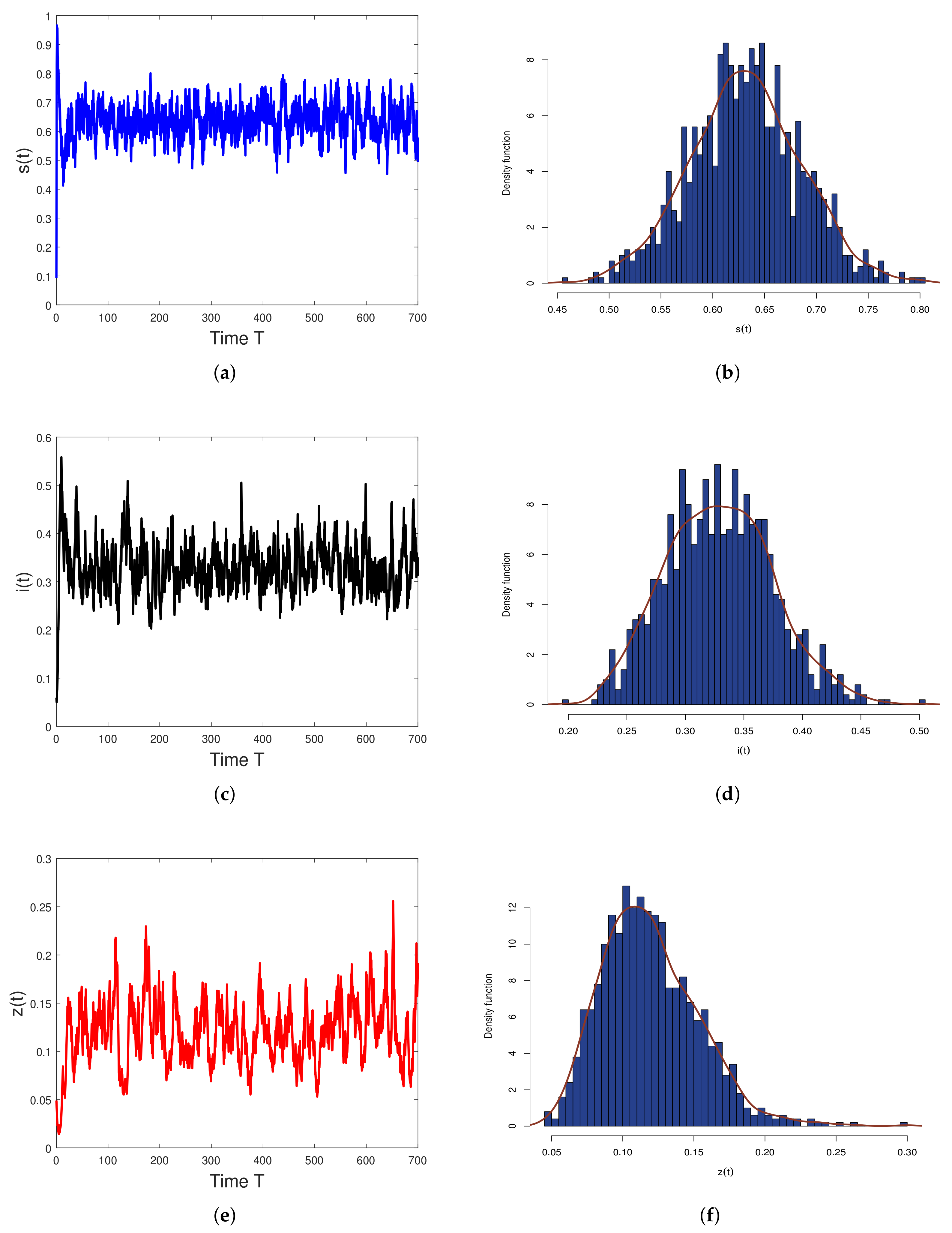
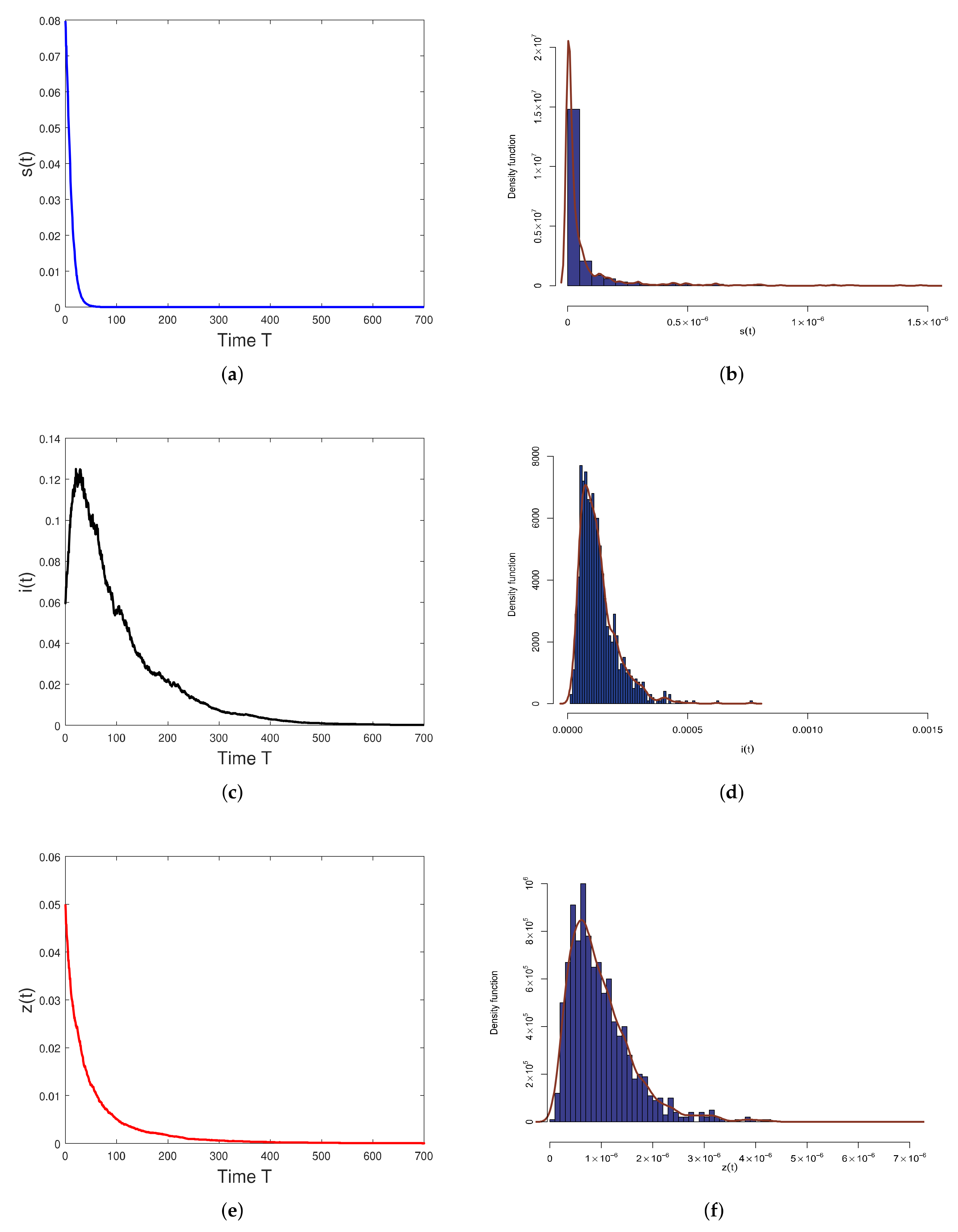
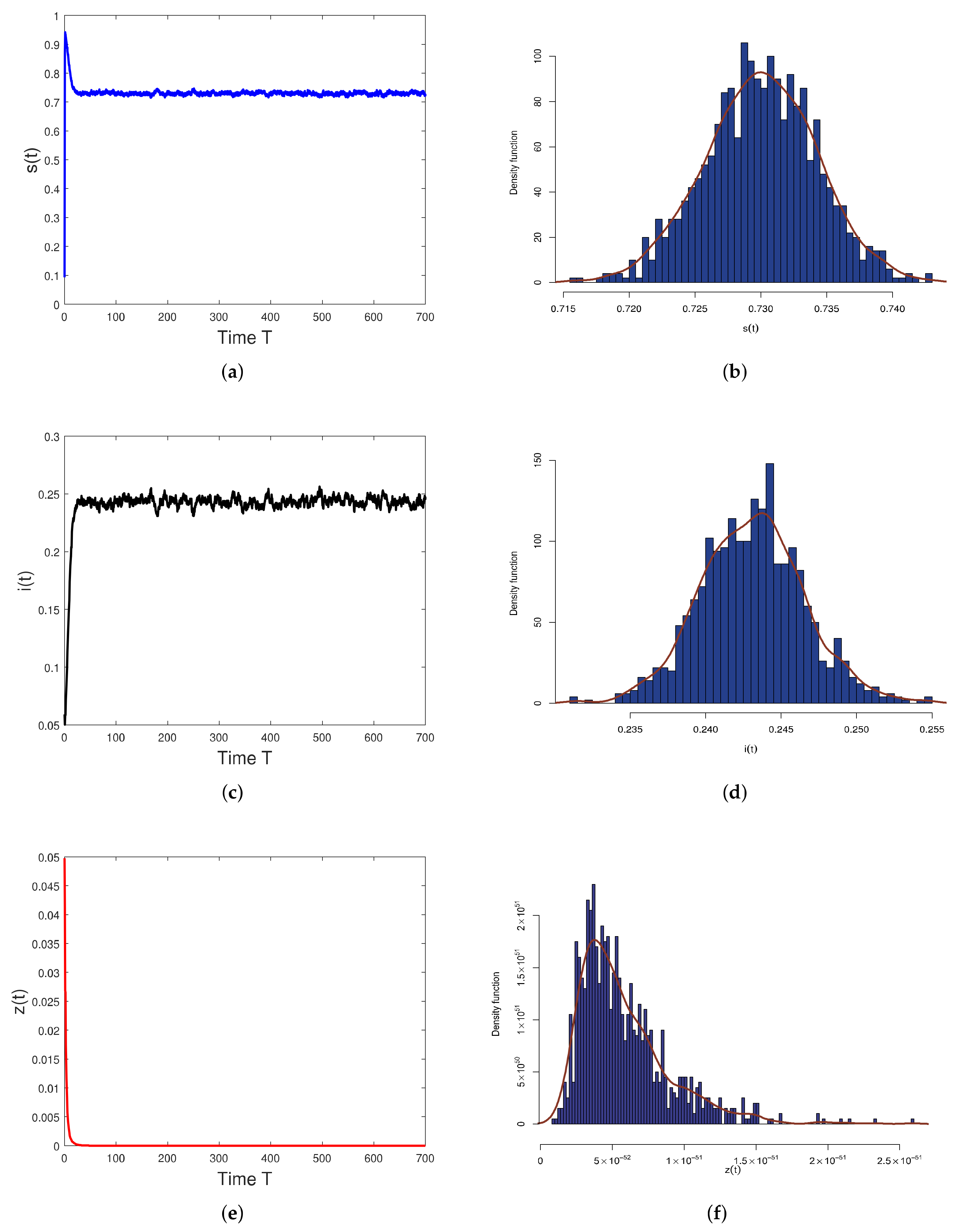
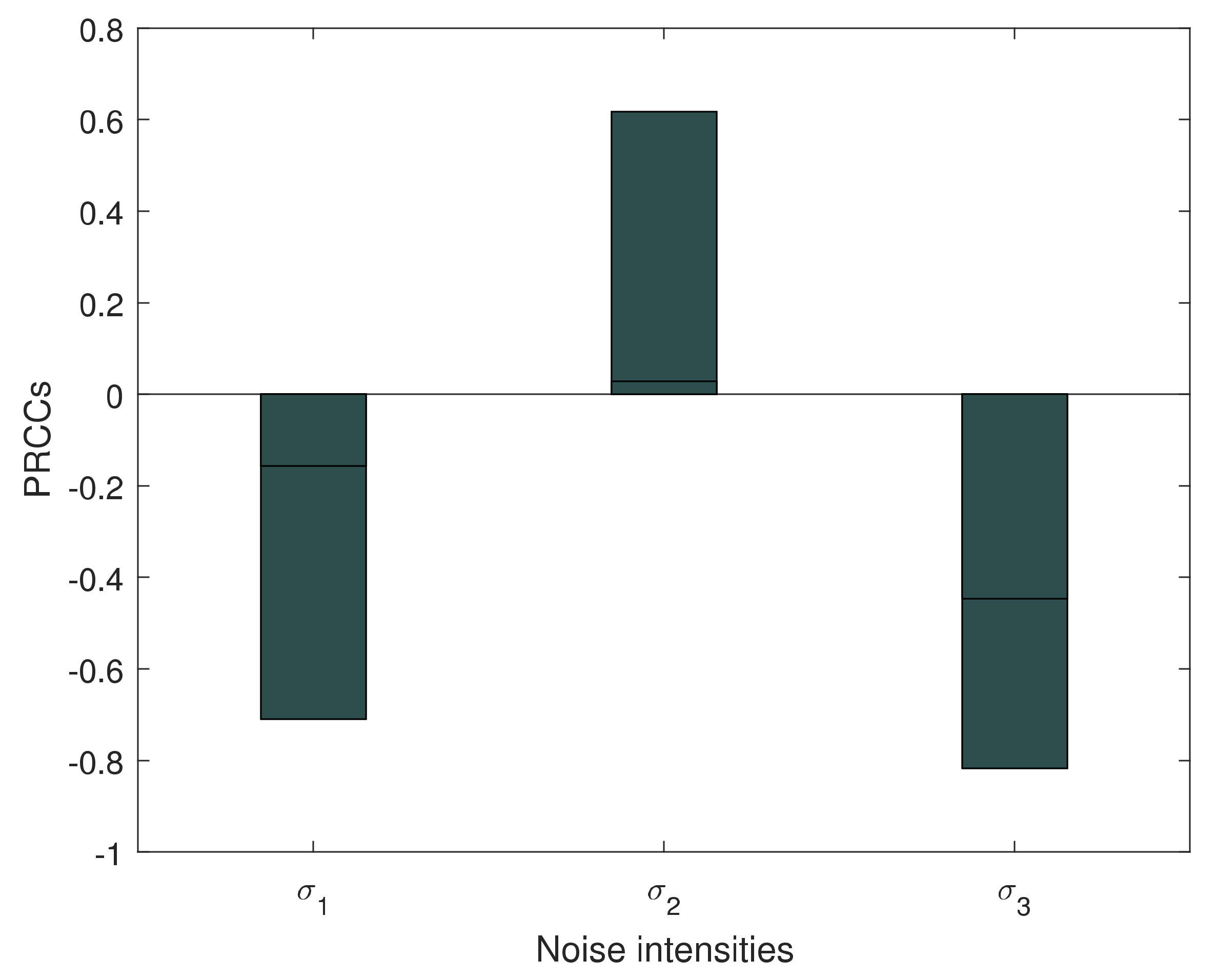
5. Numerical Simulations

In this section, by utilizing Milstein’s higher-order method [42], we will make some numerical examples to investigate the behavior of model (2) and illustrate the effects of environmental noises on the survival of plankton, which are performed by using MATLAB and R software.

Example 1.

We firstly provide the numerical simulation of the coexistence of susceptible phytoplankton $s\left(t\right)$, infected phytoplankton $i\left(t\right)$, and zooplankton $z\left(t\right)$. Under the parameter values in

Table 1. The parameter values and sources.

Parameter	Value	Reference
a	8	[9]
$l_1$	$0.011$	[19]
$l_2$	$1.5$	Assumed
$b_1$	$0.4$	[9]
n	$0.1$	Assumed
$b_2$	$0.45$	[9]

and ${\sigma }_i=0.01$$(i=1,2,3,)$ the stochastic paths of $s\left(t\right)$, $i\left(t\right)$, and $z\left(t\right)$ reveal that the susceptible phytoplankton, infected phytoplankton, and zooplankton are persistent in the mean with probability one. Based on 1000 sample paths, we obtain the probability densities for $s\left(t\right)$, $i\left(t\right)$, and $z\left(t\right)$, as shown in Figure 1a–f.

Example 2.

Choose the parameters $a=0.0015,$$l_1=0.01,$$l_2=0.05,$$b_1=0.0067,$$n=0.21,$$b_2=0.00775,$${\sigma }_1=0.012,$${\sigma }_2=0.02$, and ${\sigma }_3=0.013$, respectively. It is easy to verify that the condition for the first assertion in Theorem 2 is not satisfied; that is, $a-\frac{{\sigma }_1^2}{2}=0.014>0$. However, $s\left(t\right)$, $i\left(t\right)$, and $z\left(t\right)$ exponentially tend to zero with probability one. It indicates that the condition of the extinction for the toxin-producing phytoplankton–zooplankton system in Theorem 2 is sufficient and not necessary. As shown in Figure 2, the toxin-producing phytoplankton–zooplankton system would die out.

Example 3.

Choose $n=0.001,$$b_2=0.95$, ${\sigma }_1=0.01$, ${\sigma }_2=0.31$, and ${\sigma }_3=0.01$ but the rest of the parameters are taken from Table 1. By calculating, it can be obtained that $a-\frac{{\sigma }_1^2}{2}=9>0$, $1-b_2-\frac{{\sigma }_1^2}{2}-\frac{{\sigma }_2^2}{2}=0.0019>0$, and $l_1-n=0.01>0$, which indicate that the conditions for the second assertion in Theorem 2 are not satisfied. However, as Figure 3a–f show, $s\left(t\right)$ is persistent, while in the meanwhile, $i\left(t\right)$ and $z\left(t\right)$ would be extinct with probability one, which suggests that the condition of the second assertion in Theorem 2 may be too strong for the persistence only for susceptible phytoplankton but the extinction for infected phytoplankton and zooplankton in the aquatic system.

From the Examples 2 and 3, it can be deduced that the susceptible phytoplankton might be either persistent or extinct if condition $a>\frac{{\sigma }_1^2}{2}$ holds, which also implies that even though the self-growth of phytoplankton is relatively rapid and the effect of environmental noise is small, the phytoplankton and zooplankton system may be extinct or partially extinct. The survival of the phytoplankton and zooplankton system may be subject to other ecological factors, which is a very interesting question deserving our further investigation.

Example 4.

To further explore the effect of the noises intensities ${\sigma }_1$, ${\sigma }_2$, and ${\sigma }_3$ on the dynamical behavior of model (2), hereon, we mainly focus on the effect of environmental variability on the extinction time for $z\left(t\right)$ in model (2), which is more meaningful. Now, we define a random variable X to describe the time when $z\left(t\right)$ approaches zero, a.s., namely, $X\triangleq inf\left\{t\right|z\left(s\right)<{10}^{-5},a.s.,fors\ge t\}$. We will pay close attention to the dependence of X on three noise intensities ${\sigma }_1$, ${\sigma }_2$, and ${\sigma }_3$. We fix the other parameter values from Table 1, except for $b_2=0.73$ and ${\sigma }_i=0.01$ $(i=1,2,3)$. Under these parameters, $s\left(t\right)$ and $i\left(t\right)$ are persistent with probability one, while $z\left(t\right)$ is extinct with probability one, as shown in Figure 4. By using the Latin hypercube method to generate 1000 random samples of the parameter set $({\sigma }_1,{\sigma }_2,{\sigma }_3)$, we compute the partial rank correlation coefficients (PRCCs) for the average value of X over 1000 simulations with respect to each noise intensity, As illustrated in Figure 5, it can be found that these noise intensities have a significantly negative impact for the extinction time of $z\left(t\right)$ (under the significance level 0.05); moreover, the absolute value of the PRCC for ${\sigma }_3$ is the largest, which is suggested that ${\sigma }_3$ is more sensitive than the others for the extinction of $z\left(t\right)$.

6. Discussion and Conclusions

Actually, viral infection commonly exists in aquatic ecosystems. However, there are few models for viral infection in the toxin-producing phytoplankton and zooplankton systems. In this paper, we focus on a stochastic model of viral infection in a toxin-producing phytoplankton and zooplankton system due to considering many stochastic fluctuations in the phytoplankton–zooplankton system (for instance, the randomness of environmental factors).

In this paper, we investigated the stochastic boundness of the solutions for stochastic eco-epidemiological model for viral infection in the toxin-producing phytoplankton and zooplankton system. Sufficient conditions of extinction for the phytoplankton and zooplankton system and persistence in the mean for susceptible phytoplankton but extinction for infected phytoplankton and zooplankton are obtained. It is worth noting that these conditions are sufficient but not necessary, and the persistence for susceptible phytoplankton, infected phytoplankton, and zooplankton together are not obtained in the theoretical analysis, which is left for our further study. In addition, the phytoplankton live in a periodically varying environment; for instance, tidal circulation determines the mobility of aquatic organisms, and light intensity controls the rate of photosynthesis of phytoplankton. Hence, it is natural to incorporate the seasonal fluctuation into model (2) and investigate the effects of stochasticity and seasonality on the dynamic behavior for the phytoplankton and zooplankton system. Moreover, the time delay due to the gestation of zooplankton also could affect the dynamical behavior of the phytoplankton–zooplankton system. Therefore, it is interesting to consider a stochastic model of viral infection in toxin-producing phytoplankton and zooplankton system incorporating time-delays. These models are realistic but more complex, which deserves our further consideration.

References

1. Eilertsen, H.C.; Raa, J. Toxins in seawater produced by a common phytoplankter: Phaeocystis pouchetii. J. Mar. Biotechnol. 1995, 3, 115–119. [Google Scholar]
2. Sahoo, D.; Mondal, S.; Samanta, G.P. Interaction among toxic phytoplankton with viral infection and zooplankton in presence of multiple time delays. Int. J. Dyn. Control 2021, 9, 308–333. [Google Scholar] [CrossRef]
3. Beltrami, E.; Carroll, T. Modelling the role of viral disease in recurrent phytoplankton blooms. J. Math. Biol. 1994, 32, 857–919. [Google Scholar] [CrossRef]
4. Truscott, J.E.; Brindley, J. Ocean plankton population as excitable media. Bull. Math. Biol. 1994, 4, 981–998. [Google Scholar] [CrossRef]
5. Pal, R.; Basu, D.; Banerjee, M. Modelling of phytoplankton allelopathy with Monod-Haldane-type functional response—A mathematical study. BioSystems 2009, 136, 243–253. [Google Scholar] [CrossRef] [PubMed]
6. Yu, X.; Yuan, S.; Zhang, T. Asymptotic properties of stochastic nutrient-plankton food chain models with nutrient recycling. Nonlinear Anal. Hybrid Syst. 2019, 34, 209–225. [Google Scholar] [CrossRef]
7. Wang, Y.; Wang, H. Stability and selective harvesting of a phytoplankton-zooplankton System. J. Appl. Math. 2014, 2014, 684790. [Google Scholar] [CrossRef] [Green Version]
8. Luo, J. Phytoplankton-zooplankton dynamics in periodic environments taking into account eutrophication. Math. Biol. 2013, 245, 126–136. [Google Scholar] [CrossRef]
9. Sarkar, R.R.; Chattopadhayay, J. Occurrence of planktonic blooms under environmental fluctuations and its possible control mechanism-mathematical models and experimental observations. J. Theor. Biol. 2003, 224, 501–516. [Google Scholar] [CrossRef]
10. Jang, R.J.; Allen, E.J. Deterministic and stochastic nutrient-phytoplankton- zooplankton models with periodic toxin producing phytoplankton. Appl. Math. Comput. 2015, 271, 52–67. [Google Scholar] [CrossRef]
11. Chattopadhayay, J.; Sarkar, R.R.; Mandal, S. Toxinproducing plankton may act as a biological control for planktonic blooms—Field study and mathematical modelling. J. Theor. Biol. 2002, 215, 333–344. [Google Scholar] [CrossRef] [PubMed] [Green Version]
12. Fuhrman, J.A. Marine viruses and their biogeochemical and ecological effects. Nature 1999, 399, 541–548. [Google Scholar] [CrossRef] [PubMed]
13. Wommack, K.; Colwell, R. Virioplankton: Viruses in aquatic ecosystems. Microbiol. Mol. Biol. Rev. 2000, 64, 69–114. [Google Scholar] [CrossRef] [PubMed] [Green Version]
14. Suttle, C.; Chan, A. Marine cyanophages infecting oceanic and coastal strains of Synechococcus: Abundance, morphology, cross infectivity and growth characteristics. Mar. Ecol. Prog. Ser. 1993, 92, 69–109. [Google Scholar] [CrossRef]
15. Mondal, A.; Pal, A.K.; Samanta, G.P. Rich dynamics of non-toxic phytoplankton, toxic phytoplankton and zooplankton system with multiple gestation delays. Int. J. Dyn. Control 2020, 8, 112–131. [Google Scholar] [CrossRef]
16. Singh, B.; Chattopadhyay, J.; Sinha, S. A role of viral infection in a simple phytoplankton zooplankton system. J. Theor. Biol. 2004, 231, 153–166. [Google Scholar] [CrossRef]
17. Xiao, Y.; Chen, L. Modelling and analysis of a predator-prey model with disease in the prey. Math. Biosci. 2001, 171, 59–82. [Google Scholar] [CrossRef]
18. Chattopadhyay, J.; Pal, S. Viral infection on phytoplankton-zooplankton system—A mathematical model. Ecol. Model. 2002, 151, 15–28. [Google Scholar] [CrossRef]
19. Gakkhar, S.; Negi, K. A mathematical model for viral infection in toxin producing phytoplankton and zooplankton system. Appl. Math. Comput. 2006, 179, 301–313. [Google Scholar] [CrossRef]
20. Gakkhar, S.; Singh, A. A delay model for viral infection in toxin producing phytoplankton and zooplankton system. Commun. Nonlinear Sci. Numer. Simul. 2010, 15, 3607–3620. [Google Scholar] [CrossRef]
21. Thakur, N.K.; Srivastava, S.C.; Ojha, A. Dynamical study of an eco-epidemiological delay model for plankton system with toxicity. Iran. J. Sci. Technol. Trans. A 2021, 45, 283–304. [Google Scholar] [CrossRef]
22. Zhang, X.; Zhang, Q. Bifurcation analysis and control of a plankton-fish model with a distribution delay. J. Mech. Med. Biol. 2011, 11, 857–879. [Google Scholar] [CrossRef]
23. Nath, B.; Roy, P.; Das, K.P. Dynamics of nutrient-phytoplankton-zooplankton interaction in the presence of viral infection. Nonlinear Stud. 2019, 26, 197–217. [Google Scholar]
24. Nath, B.; Roy, P.; Sahani, S.K.; Maiti, S.; Daset, K. Plankton dynamics in nutrient-phytoplankton-zooplankton model with viral infection in phytoplankton. Nonlinear Stud. 2020, 27, 1–24. [Google Scholar]
25. Biswas, S.; Tiwari, P.K.; Kang, Y.; Samares, P. Effects of zooplankton selectivity on phytoplankton in an ecosystem affected by free-viruses and environmental toxins. Math. Biosci. Eng. 2019, 17, 1272–1317. [Google Scholar] [CrossRef]
26. Wei, C.; Fu, Y. Stationary distribution and periodic solution of stochastic toxin-producing phytoplankton-zooplankton systems. Complexity 2020, 2020, 4627571. [Google Scholar] [CrossRef] [Green Version]
27. Chen, Z.; Tian, Z.; Zhang, S.; Wei, C. The stationary distribution and ergodicity of a stochastic phytoplankton-zooplankton model with toxin-producing phytoplankton under regime switching. Physica A 2020, 537, 122728. [Google Scholar] [CrossRef]
28. Yu, X.; Yuan, S.; Zhang, T. Survival and ergodicity of a stochastic phytoplankton-zooplankton model with toxin-producing phytoplankton in an impulsive polluted environment. Appl. Math. Comput. 2019, 347, 249–264. [Google Scholar] [CrossRef]
29. Wang, H.; Liu, M. Stationary distribution of a stochastic hybrid phytoplankton-zooplankton model with toxin-producing phytoplankton. Appl. Math. Lett. 2020, 101, 106077. [Google Scholar] [CrossRef]
30. Ji, C.; Jiang, D.; Lei, D. Dynamical behavior of a one predator and two independent preys system with stochastic perturbations. Physica A 2019, 515, 649–664. [Google Scholar] [CrossRef]
31. Liu, C.; Yu, L.; Zhang, Q.; Li, Y. Dynamic analysis of a hybrid bioeconomic plankton system with double time delays and stochastic fluctuations. Appl. Math. Comput. 2018, 316, 115–137. [Google Scholar] [CrossRef]
32. Liu, Q.; Jiang, D.; Hayat, T.; Ahmad, B. Stationary distribution and extinction of a stochastic predator-prey model with additional food and nonlinear perturbation. Appl. Math. Comput. 2018, 320, 226–239. [Google Scholar] [CrossRef]
33. Cai, Y.; Mao, X. Stochastic prey-predator system with foraging arena scheme. Appl. Math. Model. 2018, 64, 357–371. [Google Scholar] [CrossRef] [Green Version]
34. Zhang, S.; Yuan, S.; Zhang, T. Dynamic analysis of a stochastic eco-epidemiological model with disease in predators. Stud. Appl. Math. 2022, 1–38. [Google Scholar] [CrossRef]
35. Feng, X.; Sun, J.; Wang, L.; Zhang, F.; Sun, S. Periodic Solutions for a Stochastic Chemostat Model with Impulsive Perturbation on the Nutrient. J. Biol. Syst. 2021, 29, 849–870. [Google Scholar] [CrossRef]
36. Rihan, F.A.; Alsakaji, H.J. Persistence and extinction for stochastic delay differential model of prey predator system with hunting cooperation in predators. Adv. Differ. Equ. 2020, 2020, 124. [Google Scholar] [CrossRef]
37. Rihan, F.A.; Alsakaji, H.J. Dynamics of a stochastic delay differential model for COVID-19 infection with asymptomatic infected and interacting peoples: Case study in the UAE. Results Phys. 2021, 28, 104658. [Google Scholar] [CrossRef]
38. Rihan, F.A.; Alsakaji, H.J.; Rajivganthi, C. Stochastic SIRC epidemic model with time-delay for COVID-19. Adv. Differ. Equ. 2020, 2020, 502. [Google Scholar] [CrossRef]
39. Jiang, D.; Shi, N.; Li, X. Global stability and stochastic permanence of a non-autonomous logistic equation with random perturbation. J. Math. Anal. Appl. 2008, 340, 588–597. [Google Scholar] [CrossRef] [Green Version]
40. Ikeda, N.; Watanabe, S. A comparison theorem for solutions of stochastic differential equations and its applications. Osaka J. Math. 1977, 14, 619–633. [Google Scholar]
41. Mao, X. Stochastic Differential Equations and Applications, 2nd ed.; Horwood Publishing: Chichester, UK, 2007; pp. 154–196. [Google Scholar]
42. Higham, D. An algorithmic introduction to numerical simulation of stochastic differential equations. SIAM Rev. 2001, 43, 525–546. [Google Scholar] [CrossRef]
Figure 1. Susceptible phytoplankton s ( t ) , infected phytoplankton i ( t ) , and zooplankton z ( t ) are persistent in the mean with probability one, based on the parameter values in Table 1 and σ i = 0.01 ( i = 1 , 2 , 3 ) . The initial value is ( 0.08 , 0.06 , 0.05 ) . (af) denote the evolution of a single path and the probability density curve (based on the 1000 simulations) of s ( t ) , i ( t ) , and z ( t ) , respectively.
Mathematics 10 01218 g001
Figure 2. Susceptible phytoplankton s ( t ) , infected phytoplankton i ( t ) , and zooplankton z ( t ) exponentially tend to zero with probability one, when the condition a σ 1 2 2 < 0 in the first assertion of Theorem 2 is not satisfied. Parameter values are chosen as a = 0.0015 ,   l 1 = 0.01 ,   l 2 = 0.05 ,   b 1 = 0.0067 ,   n = 0.21 ,   b 2 = 0.00775 ,   σ 1 = 0.012 ,   σ 2 = 0.02 , and σ 3 = 0.013 , respectively. The initial value is ( 0.08 , 0.06 , 0.05 ) . (af) denote the evolution of a single path and the probability density curve (based on the 1000 simulations) of s ( t ) , i ( t ) , and z ( t ) , respectively.
Mathematics 10 01218 g002
Figure 3. Susceptible phytoplankton s ( t ) is persistent; in the meanwhile, phytoplankton i ( t ) and zooplankton z ( t ) would be extinct with probability one, when the condition a σ 1 2 2 > 0 holds but 1 b 2 σ 1 2 2 σ 2 2 2 < 0 and l 1 n < 0 are not satisfied in the second assertion of Theorem 2. Parameter values are chosen as n = 0.001 ,   b 2 = 0.95 , σ 1 = 0.01 , σ 2 = 0.31 , and σ 3 = 0.01 , but the rest of the parameters are taken from Table 1. The initial value is ( 0.08 , 0.06 , 0.05 ) . (af) denote the evolution of a single path and the probability density curve (based on the 1000 simulations) of s ( t ) , i ( t ) , and z ( t ) , respectively.
Mathematics 10 01218 g003
Figure 4. Susceptible phytoplankton s ( t ) and infected phytoplankton i ( t ) are persistent in the mean with probability one, as is zooplankton z ( t ) when we select the parameter values in Table 1 except for b 2 = 0.73 and σ i = 0.01 ( i = 1 , 2 , 3 ) . The initial value is ( 0.08 , 0.06 , 0.05 ) . (af) denote the evolution of a single path and the probability density curve (based on the 1000 simulations) of s ( t ) , i ( t ) , and z ( t ) , respectively.
Mathematics 10 01218 g004
Figure 5. Partial rank correlation coefficients (PRCCs) for the average value of extinction time X over 1000 simulations for z ( t ) in model (2) with respect to σ 1 , σ 2 , and σ 3 . Under parameters b 2 = 0.73 , σ i = 0.01 ( i = 1 , 2 , 3 ) , the other parameters from Table 1, s ( t ) and i ( t ) are persistent with probability one, while z ( t ) is extinct with probability one. The initial values of the solutions are ( 0.08 , 0.06 , 0.05 ) .
Mathematics 10 01218 g005