Temperature Distribution in the Flow of a Viscous Incompressible Non-Newtonian Williamson Nanofluid Saturated by Gyrotactic Microorganisms

Abstract

The heat and mass transfer in magnetized non-Newtonian Williamson nanofluid flow, saturated by gyrotactic microorganisms due to a stretched sheet, is debated here. The rough sheet is subjected to uniform heat flux, and its velocity is proportional to its distance from the slit. Nanofluid viscosity and thermal conductivity are temperature-dependent, but microbe diffusivity and Brownian motion are concentration-dependent. Through similarity transformation, the system of modeled equations is reduced to dimensionless differential equations. We employed the shooting approach in conjunction with the Runge–Kutta scheme to obtain a solution for the physical model. For various combinations of the controlling parameters, some numerical results are found. When the generated results are compared to the existing literature, the highest settlement is found. According to numerical results, the skin-friction coefficient rises as the magnetic field and thermal conductivity parameters rise, while the opposite tendency is observed for both the slip velocity and viscosity parameters.

1. Introduction

One of the most critical requirements of many industrial technologies is ultra-high cooling. However, fundamentally low thermal conductivity is a major stumbling block in the development of energy-efficient heat transfer fluids for ultra-high-performance cooling. Sophisticated nanotechnology may create nanometer-sized mineral or nonmineral particles. Nanofluids are generated by hanging nanoparticles with a mean range of less than 100 nanometers in standard heat transfer fluids such as oil, water, and ethylene glycol. Choi [1] invented the name “nanofluids” to characterize a novel class of nanotechnology-based heat transfer fluids that outperform their host fluids or conventional particle fluid suspensions in terms of thermal characteristics. Many industrialization processes rely largely on nanofluid flow through stretched sheets, such as the manufacturing of polymer refinement, glass fibres, and the extrusion process of aerodynamics [2,3]. Following Choi and his group’s initial success, the nanofluid topic was looked into further, due to its prospective applications, by Khan and Pop [4] for a stretching sheet, by Makinde et al. [5] for stagnation point flow, by Qasim et al. [6] for an unsteady stretching sheet using Buongiorno’s model, and by Alali and Megahed [7] for Casson liquid film flow.

Because of the huge scientific breakthroughs in their implementations, non-Newtonian nanofluids have recently attracted the interest of scientists in the field of hydrodynamics everywhere across the world. The Williamson nanofluid is among the most prominent non-Newtonian nanofluids, with less viscosity as shear stress increases and features that are extremely comparable to polymeric solutions, for example [8,9,10]. Numerous investigators were motivated by this essential type of non-Newtonian nanofluid and investigated the flow of Williamson nanoliquids via various surfaces. The advantages of the MHD Williamson nanofluid flow in several industrial applications have also been highlighted by Mabood et al. [11]. The effect of solutal stratification on Williamson nanofluid flow was investigated by Khan et al. [12]. In the same topic, Loganathan and Rajan [13] investigated the impact of Joule heating on the Williamson nanofluid flow. On the other hand, Williamson nanofluid past an exponential stretching curved surface, according to Kamran et al. [14], was studied with variable thermal conductivity. Ahmed and Akbar [15] observed Williamson nanofluid flow and heat mass transfer while considering the magnetic field’s impact. The ability of gyrotactic bacteria to swim is crucial for understanding a variety of physical truths about nanofluids. Commercial and industrial fields such as biofertilizers, biofuel, oil reclamation, bio reactors, and beneficial secondary metabolites are all made with microorganisms [16,17,18]. As a result, the present research on non-Newtonian nanofluid flow containing gyrotactic organisms caused by a stretching sheet has a wide range of practical implications. Based on the preceding literature review, the motivation of this study is to go through the novel characteristics of flow and heat mass transfer for a non-Newtonian Williamson nanofluid containing nanoparticles and gyrotactic organisms flowing toward a rough stretched sheet that is subjected to a constant heat flux and a magnetic field. The slip velocity phenomenon and viscous dissipation effects are used to further modify the analysis.

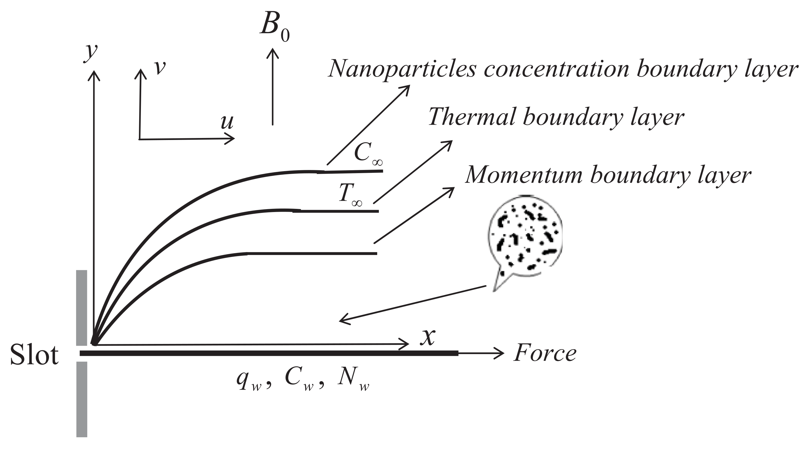
2. Mathematical Formulations

The problem design, Cartesian coordinates x and y, related velocity components u and v, and the fluid flow arrangement are all depicted in Figure 1. It is assumed that the surface is stretched through the $xy$-plane, and that this stretching process causes the Williamson nanofluid to move with velocity $ax$, where a is a constant. The gyrotactic microorganisms are thought to be enclosed in the nanofluid. Due to the existence of a magnetic field of strength $B_0$, the Williamson nanofluid is presumed to be electrically conductive.

$N_w,C_w$, and $q_w$ represent the microbe concentration, fluid concentration, and the uniform heat flux at the sheet surface, respectively, while the ambient microbe concentration, ambient fluid concentration, and ambient fluid temperature are represented by $N_{\infty },C_{\infty }$, and $T_{\infty }$, respectively. It is still assumed that the sheet in which the slip velocity is considered here is rough. The presence of the viscous dissipation phenomenon related to nanofluid motion cannot be overlooked throughout this investigation. The mathematical model for the underlying principles of mass, momentum, energy, nanoparticle volume fraction, and microbes are as follows, based on the preceding strategy’s main focuses and suppositions ([20]):

$$\frac{\partial u}{\partial x}+\frac{\partial v}{\partial y}=0,$$

(1)

$$u\frac{\partial u}{\partial x}+v\frac{\partial u}{\partial y}=\frac{1}{{\rho }_{\infty }}\frac{\partial }{\partial y}\left\{\mu \frac{\partial u}{\partial y}+\mu \frac{\Gamma }{\sqrt{2}}{\left(\frac{\partial u}{\partial y}\right)}^2\right\}-\frac{{\sigma }^{\ast }{B}_0^2}{{\rho }_{\infty }}u,$$

(2)

$$\begin{array}{cc}\hfill u\frac{\partial T}{\partial x}+v\frac{\partial T}{\partial y}=\frac{1}{{\rho }_{\infty }{c}_p}\frac{\partial }{\partial y}\left(\kappa \left(T\right)\frac{\partial T}{\partial y}\right)+\tau & \left(D_B\left(C\right)\left(\frac{\partial C}{\partial y}\frac{\partial T}{\partial y}\right)+\left(\frac{D_T}{T_{\infty }}\right){\left(\frac{\partial T}{\partial y}\right)}^2\right)\hfill \\ & +\frac{\mu }{{\rho }_{\infty }{c}_p}\left\{{\left(\frac{\partial u}{\partial y}\right)}^2+\frac{\Gamma }{\sqrt{2}}{\left(\frac{\partial u}{\partial y}\right)}^3\right\},\hfill \end{array}$$

(3)

$$u\frac{\partial C}{\partial x}+v\frac{\partial C}{\partial y}=\frac{\partial }{\partial y}\left[D_B\left(C\right)\frac{\partial C}{\partial y}\right]+\frac{D_T}{T_{\infty }}\frac{{\partial }^{2}T}{\partial y^2},$$

(4)

$$u\frac{\partial N}{\partial x}+v\frac{\partial N}{\partial y}+\frac{\tilde{b}{W}_c}{C_w-C_{\infty }}\left[\frac{\partial }{\partial y}\left(N\frac{\partial C}{\partial y}\right)\right]=\frac{\partial }{\partial y}\left[D_m\left(C\right)\frac{\partial N}{\partial y}\right],$$

(5)

where u and v are the x- and y-axis coefficients of the fluid velocity vector, $\mu$ is the nanofluid dynamic viscosity, ${\sigma }^{\ast }$ is electrical conductivity, $\kappa \left(T\right)$ is the fluid’s thermal conductivity, ${\rho }_{\infty }$ is the density of the nanofluid at the ambient, $\Gamma$ is the Williamson parameter, $D_B$ is the Brownian motion’s variable diffusivity, and $c_p$ is the specific heat at constant pressure. In addition, the coefficient of thermophoretic diffusion is denoted by $D_T$ and the chemotaxis factor is symbolized by $\tilde{b}$. Likewise, $W_c$ is the greatest speed at which a cell may swim and $D_m$ is the varying diffusivity of microorganisms. The investigation’s surface conditions have been simulated and are expressed as:

$$u=ax+\frac{{\lambda }_1}{{\mu }_{\infty }}\left(\mu \frac{\partial u}{\partial y}+\mu \frac{\Gamma }{\sqrt{2}}{\left(\frac{\partial u}{\partial y}\right)}^2\right),-\kappa \left(\frac{\partial T}{\partial y}\right)=q_w,aty=0,$$

(6)

$$v=0,C=C_w,N=N_{w}aty=0,$$

(7)

$$u\to 0,T\to T_{\infty },C\to C_{\infty },N\to N_{\infty },asy\to \infty ,$$

(8)

where the slip velocity factor is denoted by the symbol ${\lambda }_1$, and ${\mu }_{\infty }$ represents the ambient nanofluid viscosity. By analysis, the following are linear temperature-dependent thermal conductivity $\kappa \left(T\right)$ and nonlinear temperature-dependent nanofluid viscosity $\mu \left(T\right)$, as previously introduced by Megahed ([21]):

$$\mu \left(T\right)={\mu }_{\infty }{e}^{-\alpha \left({\kappa }_{\infty }\left(\frac{T-T_{\infty }}{q_w}\right)\sqrt{\frac{a}{{\nu }_{\infty }}}\right)},\kappa \left(T\right)={\kappa }_{\infty }\left[1+{\epsilon }_1\left({\kappa }_{\infty }\left(\frac{T-T_{\infty }}{q_w}\right)\sqrt{\frac{a}{{\nu }_{\infty }}}\right)\right],$$

(9)

where $\alpha$ is the viscosity parameter and ${\epsilon }_1$ is the thermal conductivity parameter. The change in the nanoparticle and microorganism diffusivities is approximated with the following mathematical functions, based on works by Amirsom et al. ([22]):

$$D_B\left(C\right)=d_1\left[1+{\epsilon }_2\left(\frac{C-C_{\infty }}{C_w-C_{\infty }}\right)\right],D_m\left(C\right)=d_2\left[1+{\epsilon }_3\left(\frac{C-C_{\infty }}{C_w-C_{\infty }}\right)\right],$$

(10)

where ${\epsilon }_2$ is the mass diffusivity parameter and ${\epsilon }_3$ is the microorganism diffusivity parameter. The problem’s governing model is of the partial differentiation kind; it is already a challenging problem to solve. As a result, the following dimensionless transformations are used ([23]):

$$\eta =y\sqrt{\frac{a{\rho }_{\infty }}{{\mu }_{\infty }}},u=ax{f}^{\prime }\left(\eta \right),v=-\sqrt{\frac{a}{{\rho }_{\infty }}{\mu }_{\infty }}f\left(\eta \right),\theta \left(\eta \right)={\kappa }_{\infty }\left(\frac{T-T_{\infty }}{q_w}\right)\sqrt{\frac{a}{{\nu }_{\infty }}}.$$

(11)

Likewise, both the nanoparticle concentration and the microorganism concentration fields are simplified via the following dimensionless quantities ([19]):

$$\varphi \left(\eta \right)=\frac{C-C_{\infty }}{C_w-C_{\infty }},\chi \left(\eta \right)=\frac{N-N_{\infty }}{N_w-N_{\infty }}.$$

(12)

In light of the aforementioned acceptable dimensionless relationships, the governing model for the problem is revealed to be a novel system of highly nonlinear, multi-degree ordinary differential equations, as follows:

$$\left(\left(1+W_e{f}^{″}\right)f^{‴}-\alpha {\theta }^{\prime }{f}^{″}\left(1+\frac{W_e}{2}{f}^{″}\right)\right)e^{-\alpha \theta }+f{f}^{″}-f^{{}^{\prime }2}-M{f}^{\prime }=0,$$

(13)

$$\frac{1}{Pr}\left((1+{\epsilon }_1\theta ){\theta }^{″}+{\epsilon }_1{\theta }^{{}^{\prime }2}\right)+f{\theta }^{\prime }+Nt{\left({\theta }^{\prime }\right)}^2+Nb(1+{\epsilon }_2\varphi ){\theta }^{\prime }{\varphi }^{\prime }+Ec\left(f^{{}^{″}2}+\frac{W_e}{2}{f}^{{}^{″}3}\right)e^{-\alpha \theta }=0,$$

(14)

$$\left(1+{\epsilon }_2\varphi \right){\varphi }^{″}+Scf{\varphi }^{\prime }+{\epsilon }_2{\varphi }^{{}^{\prime }2}+\frac{Nt}{Nb}{\theta }^{″}=0,$$

(15)

$$\left(1+{\epsilon }_3\varphi \right){\chi }^{″}+{\epsilon }_3{\varphi }^{\prime }{\chi }^{\prime }+Sbf{\chi }^{\prime }-Pe\left({\varphi }^{\prime }{\chi }^{\prime }+(\sigma +\chi ){\varphi }^{″}\right)=0,$$

(16)

together with the following boundary restrictions:

$$f^{\prime }\left(0\right)=1+\lambda \left(f^{″}+\frac{W_e}{2}{f}^{{}^{″}2}\right)e^{-\alpha \theta \left(0\right)},f\left(0\right)=0,$$

(17)

$${\theta }^{\prime }\left(0\right)=\frac{-1}{1+{\epsilon }_1\theta \left(0\right)},\varphi \left(0\right)=1,\chi \left(0\right)=1,$$

(18)

$$f^{\prime }(\infty )\to 0,\theta (\infty )\to 0,\varphi (\infty )\to 0,\chi (\infty )\to 0.$$

(19)

The resulting controlling parameters can be defined as follows:

$$M=\frac{\sigma B_0^2}{a{\rho }_{\infty }},\lambda ={\lambda }_1\sqrt{\frac{a{\rho }_{\infty }}{{\mu }_{\infty }}},W_e=\Gamma x\sqrt{\frac{2a^3}{{\nu }_{\infty }}},Pr=\frac{{\mu }_{\infty }{c}_p}{{\kappa }_{\infty }},Nt=\frac{\tau D_T{q}_w}{{\kappa }_{\infty }{T}_{\infty }\sqrt{a{\nu }_{\infty }}},$$

$$Nb=\frac{\tau d_1\left(C_w-C_{\infty }\right)}{{\nu }_{\infty }},Ec=\frac{\sqrt{a}{\kappa }_{\infty }{u}_w^2}{c_p{q}_w\sqrt{{\nu }_{\infty }}},Sc=\frac{{\nu }_{\infty }}{d_1},Sb=\frac{{\nu }_{\infty }}{d_2},Pe=\frac{\tilde{b}{W}_c}{d_2} and \sigma =\frac{N_{\infty }}{N_w-N_{\infty }},$$

which are called the magnetic parameter, the slip velocity parameter, the local Weissenberg number, the Prandtl number, the thermophoresis parameter, the Brownian motion parameter, the Eckert number, the Schmidt number, the bioconvection Schmidt number, the bioconvection Peclet number, and the bioconvection parameter, respectively. The surface drag coefficient $C{f}_x$, the Nusselt number $N{u}_x$, the Sherwood number $S{h}_x$, and the nanoparticle Sherwood number $N{n}_x$, all of which have a role in determining the surface drag force, heat and mass transfer rate, and microorganism transfer rate, are defined as follows:

$$C{f}_x{Re}_x^{1/2}=-\left(f^{″}\left(0\right)+\frac{W_e}{2}{f}^{{}^{″}2}\left(0\right)\right)e^{-\alpha \theta \left(0\right)},{Re}_x^{-1/2}N{u}_x=\frac{1}{\theta \left(0\right)},$$

(20)

$${Re}_x^{-1/2}S{h}_x=-{\varphi }^{\prime }\left(0\right),{Re}_x^{-1/2}N{n}_x=-{\chi }^{\prime }\left(0\right),$$

(21)

where ${Re}_x=\frac{a{x}^2}{{\nu }_{\infty }}$ is the local Reynolds number.

3. Numerical Solution

The closed-form solutions to Equations (13)–(16) are difficult to discover since they are highly nonlinear. As a result, the shooting method, together with the Runge–Kutta scheme of order four, is used to find the solutions of these equations with boundary conditions (17)–(19) numerically, because only first-order ODEs can be solved using the Runge–Kutta approach. The governing Equations (13)–(16) are then transformed into first-order differential equations. The governing equations are rewritten in the following way for this reason:

$$f^{‴}=\frac{\alpha {\theta }^{\prime }{f}^{″}\left(1+\frac{W_e}{2}{f}^{″}\right)+e^{\alpha \theta }\left(-f{f}^{″}+f^{{}^{\prime }2}+M{f}^{\prime }\right)}{\left(1+W_e{f}^{″}\right)},$$

(22)

$${\theta }^{″}=\frac{-{\epsilon }_1{\theta }^{{}^{\prime }2}-Pr\left[f{\theta }^{\prime }+Nt{\left({\theta }^{\prime }\right)}^2+Nb(1+{\epsilon }_2\varphi ){\theta }^{\prime }{\varphi }^{\prime }+Ec\left(f^{{}^{″}2}+\frac{W_e}{2}{f}^{{}^{″}3}\right)e^{-\alpha \theta }\right]}{(1+{\epsilon }_1\theta )},$$

(23)

$${\varphi }^{″}=\frac{-\left(Scf{\varphi }^{\prime }+{\epsilon }_2{\varphi }^{{}^{\prime }2}+\frac{Nt}{Nb}{\theta }^{″}\right)}{\left(1+{\epsilon }_2\varphi \right)},$$

(24)

$${\chi }^{″}=\frac{Pe\left({\varphi }^{\prime }{\chi }^{\prime }+(\sigma +\chi ){\varphi }^{″}\right)-{\epsilon }_3{\varphi }^{\prime }{\chi }^{\prime }-Sbf{\chi }^{\prime }}{\left(1+{\epsilon }_3\varphi \right)}.$$

(25)

The preceding equations are of order three in f, order two in $\theta$, order two in $\varphi$, and order two in $\chi$. Then, nine new variables have been developed to lower the last equations into first-order ordinary differential equations that can be treated by the Runge–Kutta approach. As a result, we presume:

$$Z_1=f,Z_2=f^{\prime },Z_3=f^{″},Z_4=\theta ,Z_5={\theta }^{\prime },$$

(26)

$$Z_6=\varphi ,Z_7={\varphi }^{\prime },Z_8=\chi ,Z_9={\chi }^{\prime }.$$

(27)

Now, Equations (22)–(25) are converted to the following form using these new variables, which are defined as follows:

$$Z_1^{\prime }=Z_2,$$

(28)

$$Z_2^{\prime }=Z_3,$$

(29)

$$Z_3^{\prime }=\frac{\alpha Z_5{Z}_3\left(1+\frac{W_e}{2}{Z}_3\right)+e^{\alpha Z_4}\left(-Z_1{Z}_3+Z_2^2+M{Z}_2\right)}{\left(1+W_e{Z}_3\right)},$$

(30)

$$Z_4^{\prime }=Z_5,$$

(31)

$$Z_5^{\prime }=\frac{-{\epsilon }_1{Z}_5^2-Pr\left[Z_1{Z}_5+Nt{Z}_5^2+Nb(1+{\epsilon }_2{Z}_6)Z_5{Z}_7+Ec\left(Z_3^2+\frac{W_e}{2}{Z}_3^3\right)e^{-\alpha Z_4}\right]}{(1+{\epsilon }_1{Z}_4)},$$

(32)

$$Z_6^{\prime }=Z_7,$$

(33)

$$Z_7^{\prime }=\frac{-\left(Sc{Z}_1{Z}_7+{\epsilon }_2{Z}_7^2+\frac{Nt}{Nb}{Z}_5^{\prime }\right)}{\left(1+{\epsilon }_2{Z}_6\right)},$$

(34)

$$Z_8^{\prime }=Z_9,$$

(35)

$$Z_9^{\prime }=\frac{Pe\left(Z_7{Z}_9+(\sigma +Z_8)Z_7^{\prime }\right)-{\epsilon }_3{Z}_7{Z}_9-Sb{Z}_1{Z}_9}{\left(1+{\epsilon }_3{Z}_6\right)}.$$

(36)

In the new variables, the relevant boundary conditions are:

$$Z_1\left(0\right)=0,Z_2\left(0\right)=1+\lambda \left(Z_3\left(0\right)+\frac{W_e}{2}{Z}_3{\left(0\right)}^2\right)e^{-\alpha Z_4\left(0\right)},$$

(37)

$$Z_5\left(0\right)=\frac{-1}{1+{\epsilon }_1{Z}_4\left(0\right)},Z_6\left(0\right)=1,Z_8\left(0\right)=1,$$

(38)

$$Z_2(\infty )\to 0,Z_4(\infty )\to 0,Z_6(\infty )\to 0,Z_8(\infty )\to 0.$$

(39)

As previously stated ([24]), the shooting technique has two primary objectives: the first is to select an adequate value for the limit $\eta \to \infty$, and the second is to choose acceptable initial estimates for $Z_3\left(0\right),Z_4\left(0\right),Z_7\left(0\right)$, and $Z_9\left(0\right)$. The Runge–Kutta integration approach is then used to solve this system of first-order differential equations with initial conditions. If the absolute differences between the provided and computed values of $Z_2(\infty ),Z_4(\infty ),Z_6(\infty )$, and $Z_8(\infty )$ are lower than the error tolerance ${10}^{-7}$, the solution will converge. However, if the difference exceeds the tolerance for error, the original guesses are changed using the Newton procedure. This technique is carried out repeatedly until the criterion is met.

4. Verification of the Numerical Method

The shooting method, together with the Runge–Kutta approach, is employed here to produce the numerical solution for the proposed physical problem. To inspect the current results, at the beginning, the authenticity of the ongoing research was proved in

Table 1. Comparison of skin-friction values $C{f}_{x}R{e}^{\frac{1}{2}}$ with the results of Hayat et al. [25].

M	Hayat et al. [25]	Present Work
0	1.00000	1.000000001
1	1.41421	1.414207989
5	2.44948	2.449479804
10	3.31662	3.316624669

and

Table 2. Comparative outputs for skin-friction values $C{f}_{x}R{e}^{\frac{1}{2}}$ with the results of Mabood and Mastroberardino [26].

M	Mabood and Mastroberardino [26]	Present Work
10	3.3166247	3.316624669
50	7.1414284	7.141428353
100	10.049875	10.04988001
500	22.383029	22.38302853
1000	31.638584	31.63858342

for the skin-friction coefficient outlines $C{f}_{x}R{e}^{\frac{1}{2}}$, which exhibited excellent agreement with the previous results of Hayat et al. [25] and Mabood and Mastroberardino [26] for some assorted values of the magnetic number M when $\lambda =\alpha =0$ and $W_e=0$.

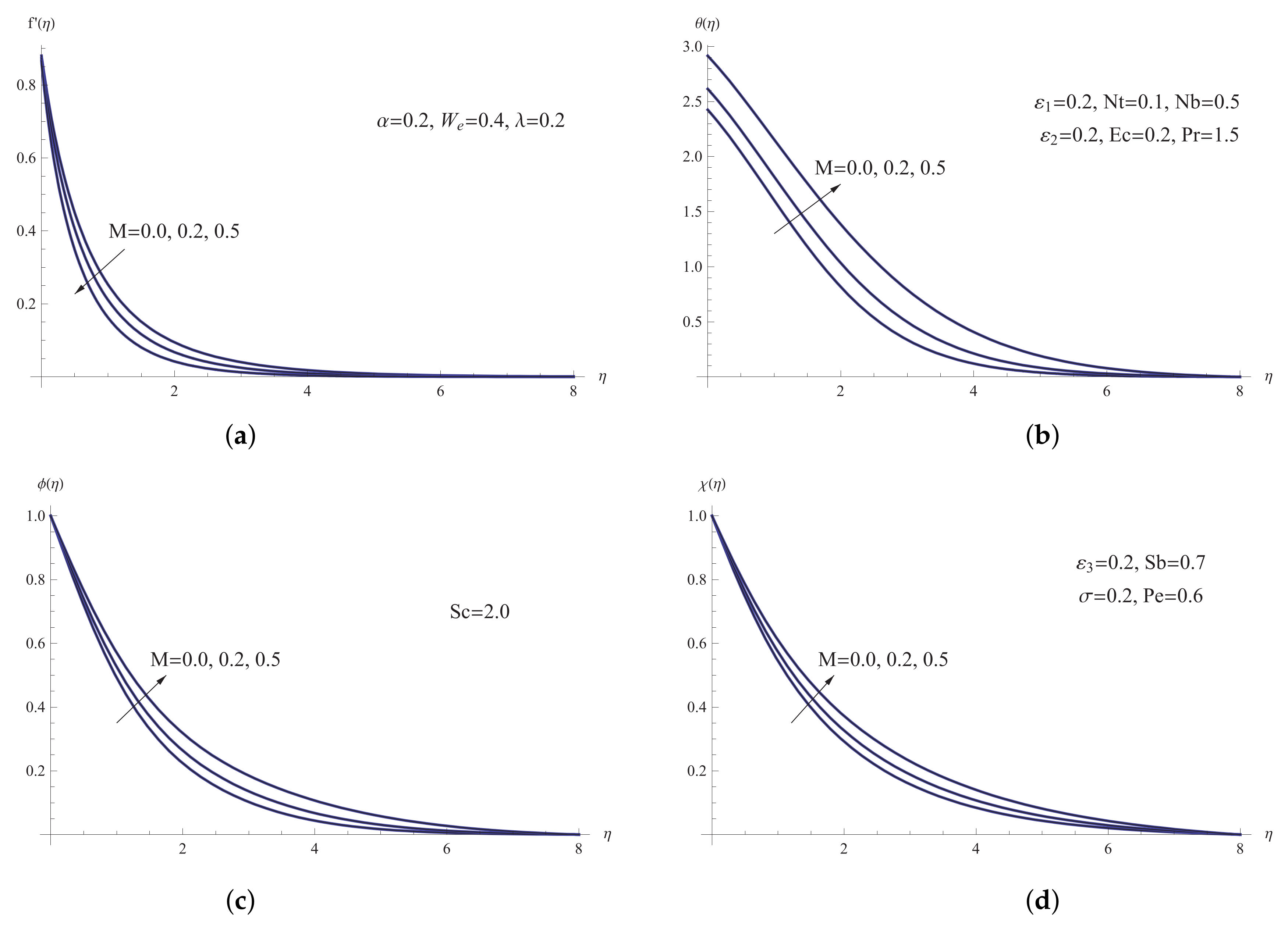
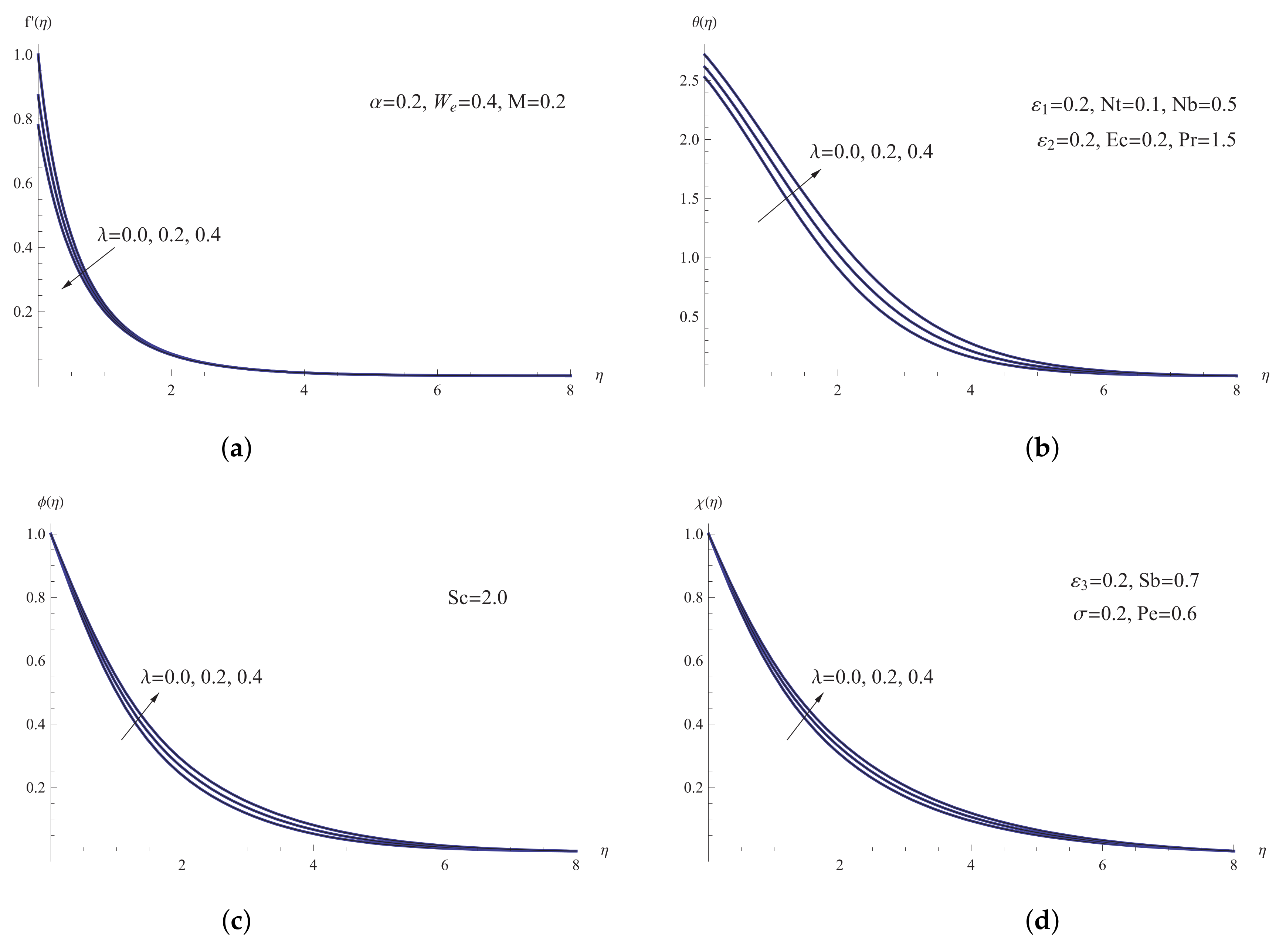
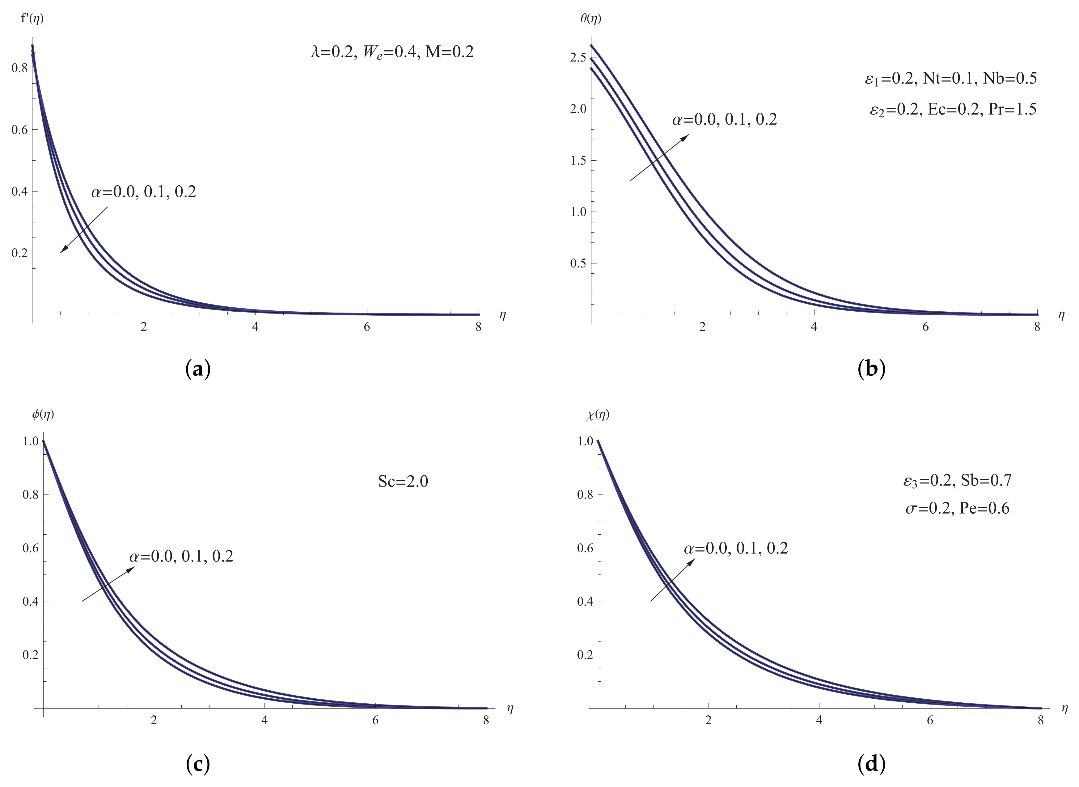
5. Results and Discussion

The graphical representations of the resulting equations, which are calculated under the effect of appropriate values of the relevant flow controlling parameters, have been presented in this section. These physical parameters are used in the ranges as $0.0\le M\le 0.5,$ $0.0\le \lambda \le 0.4,0.0\le \alpha \le 0.2,0.0\le {\epsilon }_1\le 0.5,0.0\le {\epsilon }_2\le 0.5,0.0\le {\epsilon }_3\le 0.5,$ and $0.0\le Ec\le 1.0$. As a result, for graphical display, the values of the parameters with fixed values are $\lambda =0.2,W_e=0.4,M=0.2,\alpha =0.2,Sc=2.0,Pe=0.6,\sigma =0.2,$$Sb=0.7,Pr=1.5,Nt=0.1,Nb=0.5,{\epsilon }_1=0.2,{\epsilon }_2=0.2$, and ${\epsilon }_3=0.2$. Figure 2 shows the effect of the magnetic parameter M on the dimensionless velocity $f^{\prime }\left(\eta \right)$, dimensionless temperature $\theta \left(\eta \right)$, dimensionless concentration $\varphi \left(\eta \right)$, and dimensionless microorganisms profile $\chi \left(\eta \right)$, respectively. The dimensionless velocity of Williamson nanofluids moving under the influence of a magnetic field decreases as the magnetic parameter increases, whereas the reverse tendency is observed for dimensionless temperature, dimensionless concentration, and dimensionless microorganisms. Physically, the presence of a magnetic field produces a resistive force known as the Lorentz force. This force causes the breadth of the momentum layer to narrow and the temperature of the thermal layer to rise.

Figure 3 depicts the effect of the slip velocity parameter $\lambda$ on the curves of nanofluid velocity, nanofluid temperature, nanofluid concentration, and nanofluid microorganisms. We can see that increasing the slip velocity parameter significantly dampens the nanofluid flow in these plots. Further, as they approach the free stream, the temperature profiles, concentration profiles, and motile microbe species concentration all show smoothness, and they all show enhanced behavior when the same parameter $\lambda$ is increased. Furthermore, the validation of the behavior of the velocity distribution under the impact of the slip velocity parameter is confirmed by recalling the study of Khan et al. [27].

For various viscosity factors $\alpha$, Figure 4 shows the evolution of nanoparticle velocity $f^{\prime }\left(\eta \right)$, nanoparticle temperature $\theta \left(\eta \right)$, nanoparticle concentration $\varphi \left(\eta \right)$, and nanoparticle microorganism species concentration $\chi \left(\eta \right)$ profiles. In these graphs, an increase in the viscosity parameter leads to a large rise in nanoparticle temperature, nanoparticle concentration, and nanoparticle microbe species concentration, although the nanoparticle velocity profiles show the opposite tendency. Physically, the temperature-dependent nanofluid viscosity is a cause of thermal energy generation, which raises both the sheet temperature and the temperature distribution.

The effect of the thermal conductivity parameter ${\epsilon }_1$ on the velocity $f^{\prime }\left(\eta \right)$, temperature $\theta \left(\eta \right)$, concentration $\varphi \left(\eta \right)$, and microbe species concentration $\chi \left(\eta \right)$ profiles is shown in Figure 5. It has been discovered that increasing the thermal conductivity parameter causes a modest rise in the thickness of the boundary layer as well as the Williamson nanofluid velocity. It has also been determined that temperature, concentration, and microbe species concentration are all found to be damped more when the same parameter ${\epsilon }_1$ is used. As a result, it may be argued that nanofluids with high thermal conductivity parameters play a key role in cooling processes.

Figure 6 elucidates the physical aspects’ impact of the mass diffusivity parameter ${\epsilon }_2$ on both the concentration $\varphi \left(\eta \right)$ and microbe species concentration $\chi \left(\eta \right)$ profiles, respectively. Clearly, both $\varphi \left(\eta \right)$ and $\chi \left(\eta \right)$ present an enhancing variation with the presence of the mass diffusivity parameter ${\epsilon }_2$. Likewise, Figure 7a depicts the variations in the temperature profile $\theta \left(\eta \right)$ as a function of ${\epsilon }_2$. When the mass diffusivity value ${\epsilon }_2$ is increased, the magnitude of the sheet temperature $\theta \left(0\right)$ is clearly restricted, and it is dramatically intensified as this parameter is increased.

The changes in the microbe species concentration profile $\chi \left(\eta \right)$ as a function of the microorganism diffusivity parameter ${\epsilon }_3$ are shown in Figure 7b. It is revealed that increasing the microorganism diffusivity parameter improves the behavior of the microbe species concentration profile considerably. In terms of physics, this means that the microorganism diffusivity parameter is what causes the microbe concentration layer to thicken.

Finally, Figure 8, elucidates the impact of the Eckert number $Ec$ on the velocity $f^{\prime }\left(\eta \right)$, temperature $\theta \left(\eta \right)$, concentration $\varphi \left(\eta \right)$, and the microbe species concentration profile $\chi \left(\eta \right)$ plots, respectively. The bigger the value of $Ec$, the higher the temperature, sheet temperature $\theta \left(0\right)$, concentration, and microbe species concentration sketches. The physics underlying this is that more energy is passed from surface to fluid due to a higher viscous dissipation phenomena. Furthermore, the velocity sketch $f^{\prime }\left(\eta \right)$ decreases due to larger estimates of the Eckert number $Ec$, as seen in the same figure. The heat source resulting from the transformation of kinetic energy into internal thermal energy due to viscous stresses is accounted for by the viscous dissipation phenomena. Physically, the presence of viscous dissipation indicates the formation of thermal energy, which raises the sheet temperature, the thickness of the thermal boundary layer, and the temperature distribution.

Wall friction $C_{f_x}R{e}_x^{\frac{1}{2}}$, wall heat transfer $N{u}_{x}R{e}_x^{\frac{-1}{2}}$, wall mass transfer $S{h}_{x}R{e}_x^{\frac{-1}{2}}$, and wall microorganism transfer rate $N{n}_{x}R{e}_x^{\frac{-1}{2}}$ observations, due to the impact of the controlling factors, are provided in

Table 3. Values for $C_{f_x}R{e}_x^{\frac{1}{2}}$, $N{u}_{x}R{e}_x^{\frac{-1}{2}}$, $S{h}_{x}R{e}_x^{\frac{-1}{2}}$, and $N{n}_{x}R{e}_x^{\frac{-1}{2}}$ for various values of $M,\lambda ,\alpha$, ${\epsilon }_1,Ec,{\epsilon }_2$, and ${\epsilon }_3$, with $Pr=1.5,Sc=2.0,Pe=0.6,W_e=0.4,\sigma =0.2$, and $Sb=0.7$.

M	$\mathit{\lambda }$	$\mathit{\alpha }$	${\mathit{\epsilon }}_1$	${\mathit{\epsilon }}_2$	${\mathit{\epsilon }}_3$	$\mathit{Ec}$	${\mathit{C}}_{{\mathit{f}}_{\mathit{x}}}{\mathit{Re}}_{\mathit{x}}^{\frac{1}{2}}$	${\mathit{Nu}}_{\mathit{x}}{\mathit{Re}}_{\mathit{x}}^{\frac{-1}{2}}$	${\mathit{Sh}}_{\mathit{x}}{\mathit{Re}}_{\mathit{x}}^{\frac{-1}{2}}$	${\mathit{Nn}}_{\mathit{x}}{\mathit{Re}}_{\mathit{x}}^{\frac{-1}{2}}$
0.0	0.2	0.2	0.2	0.2	0.2	0.2	0.600491	0.412248	0.579751	0.542643
0.2	0.2	0.2	0.2	0.2	0.2	0.2	0.635508	0.382405	0.540179	0.505161
0.5	0.2	0.2	0.2	0.2	0.2	0.2	0.670821	0.343003	0.487964	0.457065
0.2	0.0	0.2	0.2	0.2	0.2	0.2	0.746086	0.395622	0.577339	0.537076
0.2	0.2	0.2	0.2	0.2	0.2	0.2	0.635508	0.382405	0.540179	0.505161
0.2	0.4	0.2	0.2	0.2	0.2	0.2	0.549154	0.367881	0.508204	0.477407
0.2	0.2	0.0	0.2	0.2	0.2	0.2	0.796625	0.418147	0.595505	0.557137
0.2	0.2	0.1	0.2	0.2	0.2	0.2	0.719606	0.402434	0.571268	0.534082
0.2	0.2	0.2	0.2	0.2	0.2	0.2	0.635508	0.382405	0.540179	0.505161
0.2	0.2	0.2	0.0	0.2	0.2	0.2	0.584102	0.285624	0.488075	0.473978
0.2	0.2	0.2	0.2	0.2	0.2	0.2	0.635508	0.382405	0.540179	0.505161
0.2	0.2	0.2	0.5	0.2	0.2	0.2	0.660554	0.459025	0.563998	0.519245
0.2	0.2	0.2	0.2	0.0	0.2	0.2	0.639832	0.392205	0.670139	0.557869
0.2	0.2	0.2	0.2	0.2	0.2	0.2	0.635508	0.382405	0.540179	0.505161
0.2	0.2	0.2	0.2	0.5	0.2	0.2	0.629451	0.369405	0.418768	0.455989
0.2	0.2	0.2	0.2	0.2	0.0	0.2	0.635508	0.382405	0.540179	0.576694
0.2	0.2	0.2	0.2	0.2	0.2	0.2	0.635508	0.382405	0.540179	0.505051
0.2	0.2	0.2	0.2	0.2	0.5	0.2	0.635508	0.382405	0.540179	0.429340
0.2	0.2	0.2	0.2	0.2	0.2	0.0	0.647482	0.411927	0.540144	0.507516
0.2	0.2	0.2	0.2	0.2	0.2	0.5	0.617545	0.345041	0.539406	0.501026
0.2	0.2	0.2	0.2	0.2	0.2	1.0	0.587747	0.296533	0.536391	0.493252

as tabular data. Table 3 shows that as the thermal conductivity parameter, magnetic number, and Eckert number are increased, the wall friction values tend to climb; however, they decrease if the slip parameter and viscosity parameter are increased. The recorded data also anticipates that the thermal conductivity parameter has a significant increasing effect on the wall friction, wall heat transfer, wall mass transfer, and wall microorganism transfer rate for the studied Williamson nanofluid, whereas the mass diffusivity parameter has a significant decreasing effect. Likewise, the mass transfer rate is found to lower as the viscosity and magnetic and slip velocity parameters are elevated. The behavior of the wall microorganism transfer rate diminishes when the microorganism diffusivity parameter is increased, although the behavior of the wall mass transfer slightly decreases with the same parameter.

6. Conclusions

This research sets the way for a well-described systematic theoretical evaluation of non-Newtonian nanofluid, in order to model them most effectively. The scientific novelty of the current study can be highlighted through the simultaneous impact of the viscous dissipation and slip velocity phenomenon in the attendance of a constant heat flux on the flow and heat mass transfer of the Williamson nanofluids with gyrotactic microorganisms. The analysis of the proposed problem is conducted in the attendance of a constant heat flux, viscous dissipation, and slip velocity phenomenon along the boundary. With the help of tables and graphs, we have numerically depicted the impacts of various parameters on physical factors. The following are the responses to the above-mentioned inquiries, along with some noteworthy highlights:

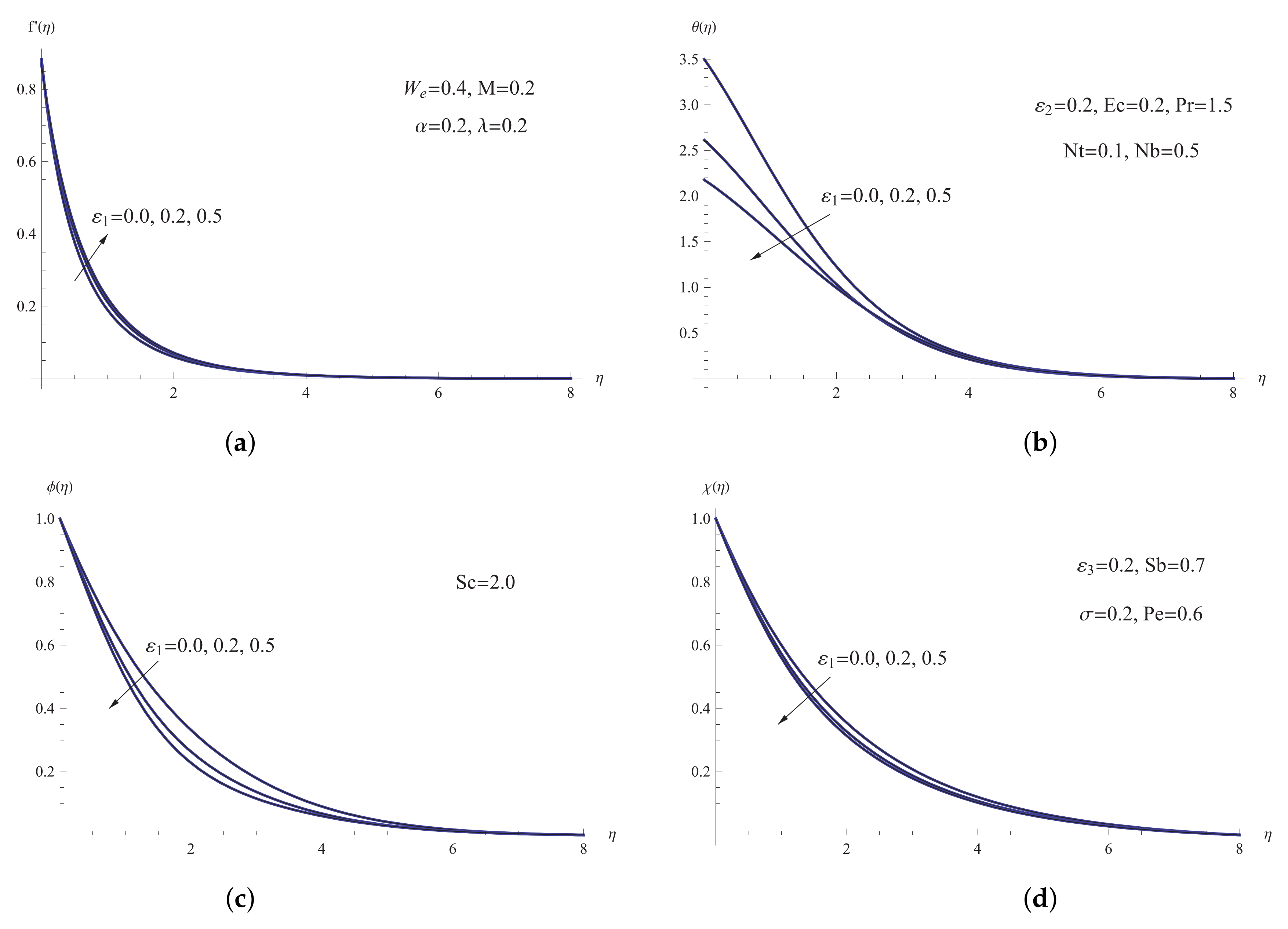
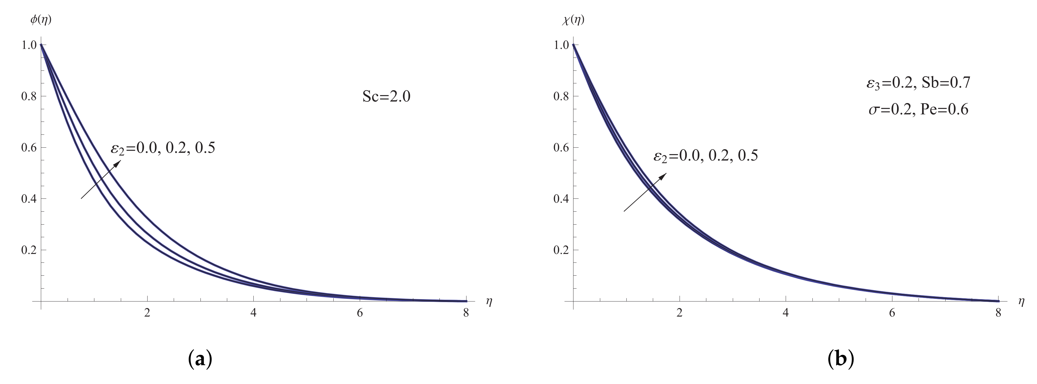
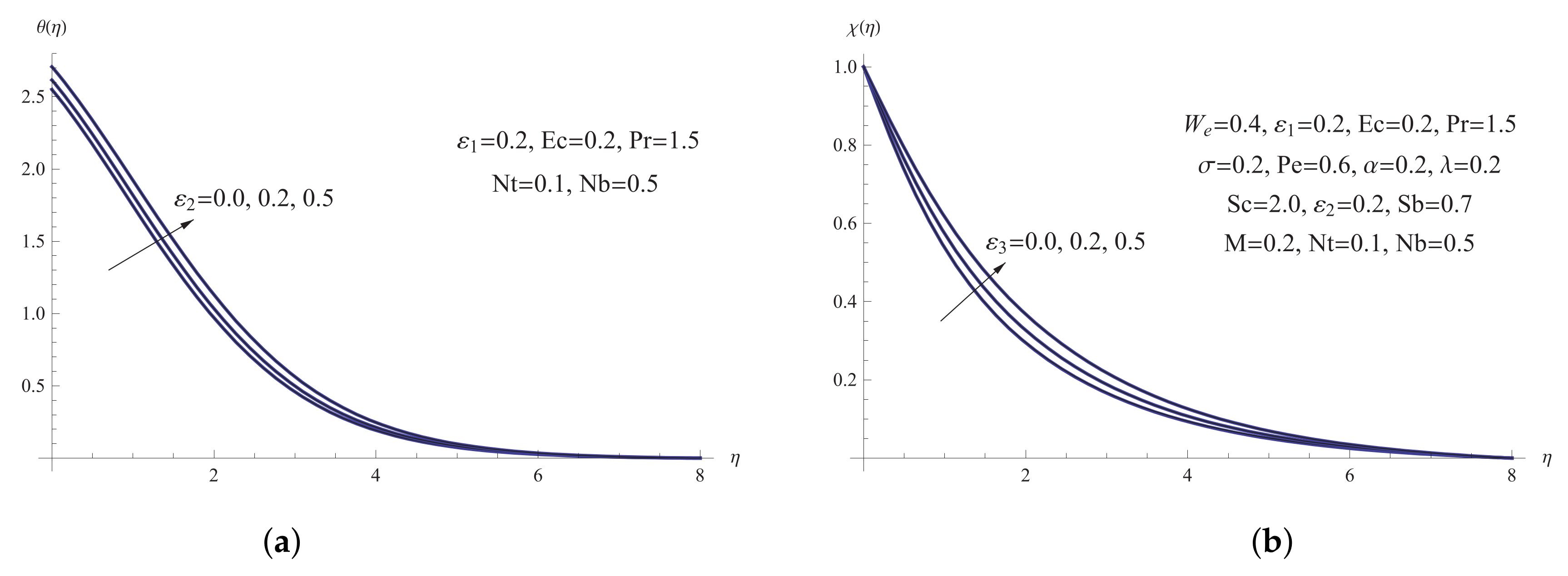
• The fluid temperature and thickness of the thermal boundary layer are improved by higher values of Eckert number, mass diffusivity parameter, viscosity parameter, and slip velocity parameter;
• The slip velocity parameter, viscosity parameter, and magnetic number are responsible for dropping the rate of mass heat transfer;
• The viscous forces are created by boosting the magnetic number, Eckert number, and viscosity parameter, causing a reduction in fluid velocity;
• The microorganism transfer rate is reduced by greater values of the magnetic number, slip velocity parameter, Eckert number, and viscosity parameter, whereas the thermal conductivity parameter improves it;
• The Nusselt number lowers when the magnetic number, slip velocity parameter, and viscosity parameter are estimated more accurately;
• In the future, we intend to expand on this research by looking into mass flux and how it affects flow through porous media.

References

1. Choi, U.S.S. Enhancing thermal conductivity of fluids with nanoparticles, developments and application of non-Newtonian flows. ASME J. Heat Transf. 1995, 66, 99–105. [Google Scholar]
2. Choi, S.U.S.; Zhang, Z.G.; Yu, W.; Lockwood, F.E.; Grulke, E.A. Anomalous thermal conductivity enhancement in nanotube suspensions. Appl. Phys. Lett. 2001, 79, 2252–2254. [Google Scholar] [CrossRef]
3. Vasu, V.; Rama Krishna, K.; Kumar, A.C.S. Analytical prediction of forced convective heat transfer of fluids embedded with nanostructured materials (nanofluids). Pramana J. Phys. 2007, 69, 411–421. [Google Scholar] [CrossRef]
4. Khan, W.A.; Pop, I. Boundary-layer flow of a nanofluid past a stretching sheet. Int. J. Heat Mass Transf. 2010, 53, 2477–2483. [Google Scholar] [CrossRef]
5. Makinde, O.D.; Khan, W.A.; Khan, Z.H. Buoyancy effects on MHD stagnation point flow and heat transfer of a nanofluid past a convectively heated stretching/shrinking sheet. Int. J. Heat Mass Transf. 2013, 62, 526–533. [Google Scholar] [CrossRef]
6. Qasim, M.; Khan, Z.H.; Lopez, R.J.; Khan, W.A. Heat and mass transfer in nanofluid over an unsteady stretching sheet using Buongiorno’s model. Eur. Phys. J. Plus 2016, 131, 16. [Google Scholar] [CrossRef]
7. Alali, E.; Megahed, M.A. MHD dissipative Casson nanofluid liquid film flow due to an unsteady stretching sheet with radiation influence and slip velocity phenomenon. Nanotechnol. Rev. 2022, 11, 463–472. [Google Scholar] [CrossRef]
8. Nadeem, S.; Hussain, S.T. Flow and heat transfer analysis of Williamson nanofluid. Appl. Nanosci. 2014, 4, 1005–1012. [Google Scholar] [CrossRef] [Green Version]
9. Krishnamurthy, M.R.; Prassanakumara, B.C.; Gireesha, B.J.; Gorla, R.S.R. Effect of chemical reaction on MHD boundary layer flow and melting heat transfer of Williamson nanofluid in porous medium. Eng. Sci. Technol. Int. J. 2016, 19, 53–61. [Google Scholar] [CrossRef] [Green Version]
10. Khan, M.; Malik, M.Y.; Salahuddin, T.; Rehman, K.U.; Naseer, M.; Khan, I. Numerical study for MHD peristaltic flow of Williamson nanofluid in an endoscope with partial slip and Journal wall properties. Int. Heat Mass Transf. 2017, 114, 1181–1187. [Google Scholar]
11. Mabood, F.; Ibrahim, S.M.; Lorenzini, G.; Lorenzini, E. Radiation effects on Williamson nanofluid flow over a heated surface with magnetohydrodynamics. Int. J. Heat Technol. 2017, 35, 196–204. [Google Scholar] [CrossRef]
12. Khan, M.; Salahuddin, T.; Malik, M.Y.; Mallawi, F.O. Change in viscosity of Williamson nanofluid flow due to thermal and solutal stratification. Int. J. Heat Mass Transf. 2018, 126, 941–948. [Google Scholar] [CrossRef]
13. Loganathan, K.; Rajan, S. An entropy approach of Williamson nanofluid flow with Joule heating and zero nanoparticle mass flux. J. Therm. Anal. Calorim. 2020, 141, 2599–2612. [Google Scholar] [CrossRef]
14. Kamran, A.; Tanvir, A.; Taseer, M.; Metib, A. Heat transfer characteristics of MHD flow of Williamson nanofluid over an exponential permeable stretching curved surface with variable thermal conductivity. Case Stud. Therm. Eng. 2021, 28, 101544. [Google Scholar]
15. Ahmed, K.; Akbar, T. Numerical investigation of magnetohydrodynamics Williamson nanofluid flow over an exponentially stretching surface. Adv. Mech. Eng. 2021, 13, 16878140211019875. [Google Scholar] [CrossRef]
16. Waqas, S.H.; Khan, S.U.; Imran, M.; Bhatti, M.M. Thermally developed Falkner-Skan bioconvection flow of a magnetized nanofluid in the presence of a motile gyrotactic microorganism: Buongiorno’s nanofluid model. Phys. Scr. 2019, 94, 115304. [Google Scholar] [CrossRef]
17. Hayat, T.; Bashir, Z.; Qayyum, S.; Alsaedi, A. Nonlinear radiative flow of nanofluid in presence of gyrotactic microorganisms and magnetohydrodynamic. Int. J. Numer. Methods Heat Fluid Flow 2019, 29, 3039–3055. [Google Scholar] [CrossRef]
18. Khan, S.U.; Shehzad, S.A.; Ali, N. Bioconvection flow of magnetized Williamson nanoliquid with motile organisms and variable thermal conductivity. Appl. Nanosci. 2020, 10, 3325–3336. [Google Scholar] [CrossRef]
19. Sankad, G.; Ishwar, M.; Dhange, M. Varying wall temperature and thermal radiation effects on MHD boundary layer liquid flow containing gyrotactic microorganisms. Partial. Differ. Equ. Appl. Math. 2021, 4, 100092. [Google Scholar]
20. Yusuf, T.A.; Mabood, F.; Prasannakumara, B.C.; Ioannis, E.S. Magneto-bioconvection flow of Williamson nanofluid over an inclined plate with gyrotactic microorganisms and entropy generation. Fluids 2021, 6, 109. [Google Scholar] [CrossRef]
21. Megahed, A.M. Improvement of heat transfer mechanism through a Maxwell fluid flow over a stretching sheet embedded in a porous medium and convectively heated. Math. Comput. Simul. 2021, 187, 97–109. [Google Scholar] [CrossRef]
22. Amirsom, N.; Uddin, M.; Ismail, A. Three dimensional stagnation point flow of bionanofluid with variable transport properties. Alex. Eng. J. 2016, 55, 1983–1993. [Google Scholar] [CrossRef]
23. Shamshuddin, M.D.; Thirupathi, T.; Satya Narayana, P.V. Micropolar fluid flow induced due to a stretching sheet with heat source/sink and surface heat flux boundary condition effects. J. Appl. Comput. Mech. 2019, 5, 816–826. [Google Scholar]
24. Zhou, S.S.; Khan, M.I.; Qayyum, S.; Prasannakumara, B.C.; Kumar, R.N.; Khan, S.U.; Gowda, R.P.; Chu, Y.M. Nonlinear mixed convective Williamson nanofluid flow with the suspension of gyrotactic microorganisms. Int. J. Mod. Phys. B 2021, 35, 2150145. [Google Scholar] [CrossRef]
25. Hayat, T.; Hussain, Q.; Javed, T. The modified decomposition method and Pade approximants for the MHD flow over a non-linear stretching sheet. Nonlinear Anal. Real World Appl. 2009, 10, 966–973. [Google Scholar] [CrossRef]
26. Mabood, F.; Mastroberardino, A. Melting heat transfer on MHD convective flow of a nanofluid over a stretching sheet with viscous dissipation and second order slip. J. Taiwan Inst. Chem. Eng. 2015, 57, 62–68. [Google Scholar] [CrossRef]
27. Khan, M.I.; Khan, W.A.; Waqas, M.; Kadry, S.; Chu, Y.M.; Nazeer, M. Role of dipole interactions in Darcy-Forchheimer first-order velocity slip nanofluid flow of Williamson model with Robin conditions. Appl. Nanosci. 2020, 10, 5343–5350. [Google Scholar] [CrossRef]
Figure 1. Schematic for the physical model [19].
Mathematics 10 01256 g001
Figure 2. (a) f ( η ) for various M. (b) θ ( η ) for various M. (c) ϕ ( η ) for various M. (d) χ ( η ) for various M.
Mathematics 10 01256 g002
Figure 3. (a) f ( η ) for various λ . (b) θ ( η ) for various λ . (c) ϕ ( η ) for various λ . (d) χ ( η ) for various λ .
Mathematics 10 01256 g003
Figure 4. (a) f ( η ) for various α . (b) θ ( η ) for various α . (c) ϕ ( η ) for various α . (d) χ ( η ) for various α .
Mathematics 10 01256 g004
Figure 5. (a) f ( η ) for various ε 1 . (b) θ ( η ) for various ε 1 . (c) ϕ ( η ) for various ε 1 . (d) χ ( η ) for various ε 1 .
Mathematics 10 01256 g005
Figure 6. (a) ϕ ( η ) for various ε 2 . (b) χ ( η ) for various ε 2 .
Mathematics 10 01256 g006
Figure 7. (a) θ ( η ) for various ε 2 . (b) χ ( η ) for various ε 3 .
Mathematics 10 01256 g007
Figure 8. (a) f ( η ) for various E c . (b) θ ( η ) for various E c . (c) ϕ ( η ) for various E c . (d) χ ( η ) for various E c .
Mathematics 10 01256 g008