
Automatic Fingerprint Classification Using Deep Learning Technology (DeepFKTNet)


Abstract
:1. Introduction
- We developed an efficient automatic method for classifying cross-sensor fingerprints based on a CNN model.
- We proposed a technique for the custom-designed building of a CNN model, which automatically determines the architecture of the model using the class discriminative information from fingerprints. The layers and their respective filters of an adaptive CNN model are customized using FKT, and the ratio of the traces of the between-class scatter matrix, and the within-class scatter matrix.
- We thoroughly evaluated the proposed method on two datasets. The proposed fingerprint classification scheme is quick, accurate, and performs well with noisy fingerprints obtained using live scan devices as well as cross-sensor fingerprints.
2. Proposed Method
2.1. Problem Formulation
2.2. Adaptive CNN Model
2.2.1. Selection of Representative Fingerprints
2.2.2. Design of the Main DeepFKTNet Architecture
| Algorithm 1: Design of the main DeepFKTNet Architecture | |
| Input: The set X = {X1, X2, …, XC}, where Xi = {RFj, j = 1, 2, 3, …, ni} is the set of representative fingerprints of ith class. | |
| Output: The main DeepFKTNet Architecture. | |
| Step 1: | Initialize DeepFKTNet with input layer and set w = 7, h = 7, d = 1, and m (the number of filters) = 0 for the first layer; PTR (previous TR) = 0. |
| Step 2: | For i = 1, 2, 3,…, C |
| Compute = RFj, for each | |
| Step 3: | For |
| Ai = ∅ | |
| For each | |
| Extract patches of size w × h with stride 1 from , vectorize them | |
| into vectors of dimension and append to Ai. | |
| Step 4: | Using , compute |
| -between-class scatter matrix , where is an matrix with all ones. | |
| -within-class scatter matrices | |
| Step 5: | Diagonalize the sum and transform the scatter matrices |
| using the transform matrix . i.e., , | |
| Step 6: | Compute eigenvectors of such that |
| Step 7: | For each eigenvector |
| -Reshape to a filter fk of size | |
| -Compute where | |
| -Compute the between scatter matrix SFb and within scatter matrix SFw from . | |
| -Compute the trace ratio | |
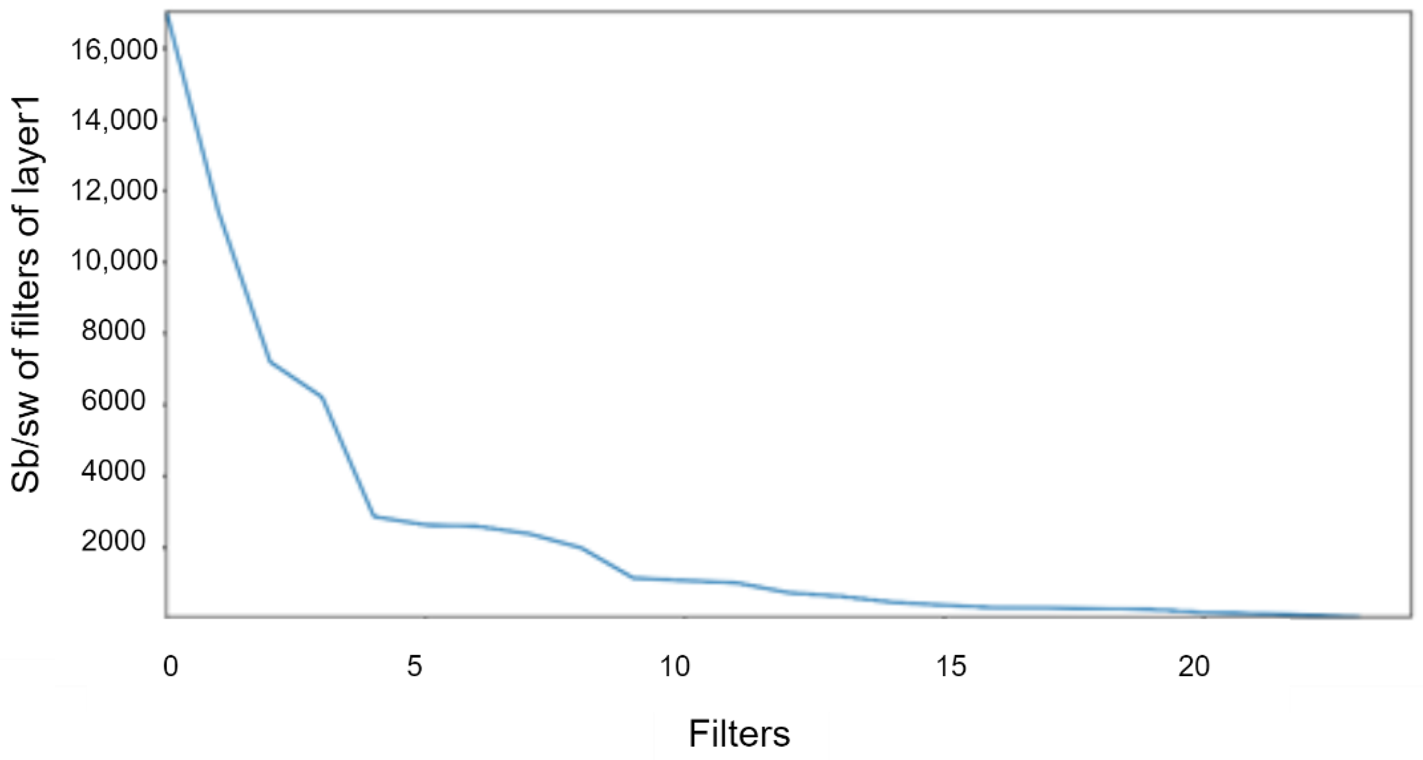
| Step 8: | Select L filters corresponding to (as shown in Figure 2 for layer 1). |
| Step 9: | Add the CONV block to DeepFKTNet with filters . Update m = m + 1. |
| Step 10: | If m = 1 or 2, add a max pool layer with pooling operation of size 2 × 2 and stride 2 to |
| Deep FKTNet. | |
| Step 11: | Compute , where = DeepFKTNet(RFj), for each |
| Step 12: | Using , compute the ratio |
| If , w = 3, h = 3, d = L and go to Step 3, otherwise stop. | |
2.3. Addition of Global Pool and Softmax Layers
2.4. Fine-Tuning the Model
2.4.1. Datasets and the Adaptive Architectures
2.4.2. Evaluation Procedure
3. Experimental Results
4. Discussions

| Paper | Method | Performance (%) | |||
|---|---|---|---|---|---|
| ACC | SE | SP | Kappa | ||
| Gupta et al. [72] 2015 | Singular point | 97.80 | - | - | - |
| Darlow et al. [73] 2017 | Minutiae and DL | 94.55 | - | - | - |
| Andono et al. [74] 2018 | Bag-of-Visual-Words | 90 | - | - | - |
| Saeed et al. [19] 2018 | statistics of D-SIFT descriptor | 97.40 | - | - | - |
| Saeed et al. [18] 2018 | Modified HOG descriptor | 98.70 | - | - | - |
| Jeon et al. [70] 2017 | Ensemble CNN model | 97.2 | - | - | - |
| Zia et al. [33] 2019 | B-DCNNs | 95.3 | |||
| Nguyen et al. [34] 2019 | CNN (tested on 3 classes of FVC2004) | 96.1 | |||
| Nahar et al. [35] 2022 | Modified LeNet (tested on FVC2004-DB1) | 99.1 | |||
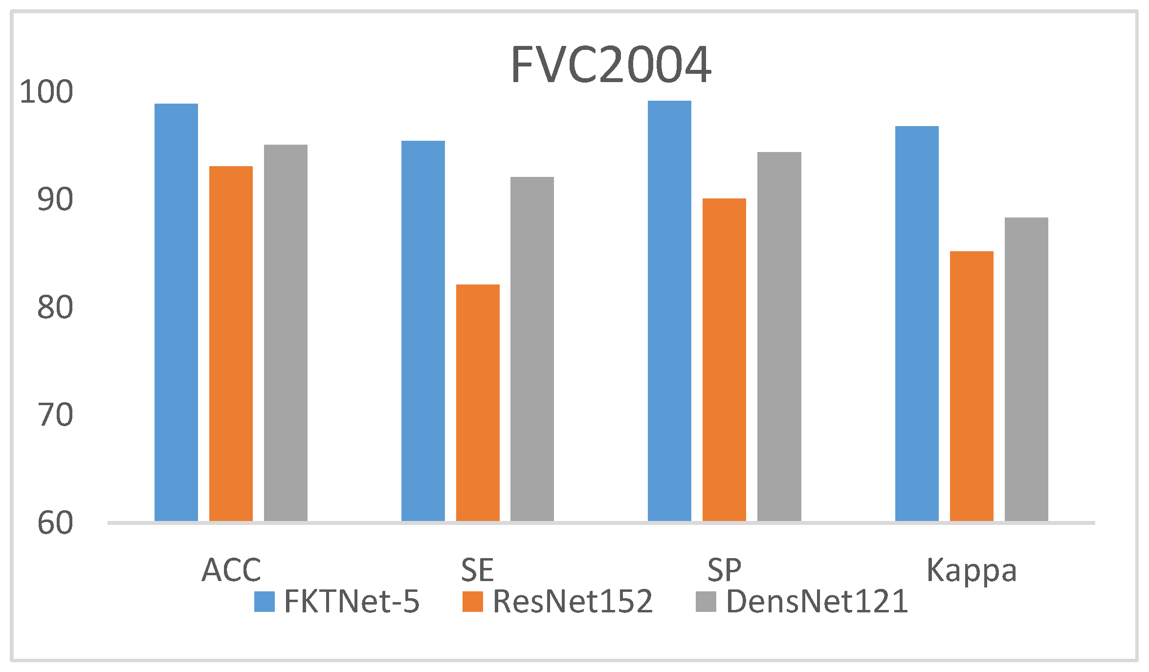
| DeepFKTNet-5 | DeepFKTNet model | 98.89 | 95.46 | 99.18 | 96.82 |
5. Conclusions
Author Contributions
Funding
Institutional Review Board Statement
Informed Consent Statement
Data Availability Statement
Conflicts of Interest
References
- Grabatin, M.; Steinke, M.; Pöhn, D.; Hommel, W. A Matrix for Systematic Selection of Authentication Mechanisms in Challenging Healthcare related Environments. In Proceedings of the 2021 ACM Workshop on Secure and Trustworthy Cyber-Physical Systems, Virtually, TN, USA, 28 April 2021; pp. 88–97. [Google Scholar]
- Maltoni, D.; Maio, D.; Jain, A.K.; Prabhakar, S. Handbook of Fingerprint Recognition; Springer Science & Business Media: Berlin/Heidelberg, Germany, 2009. [Google Scholar]
- Pandey, F.; Dash, P.; Samanta, D.; Sarma, M. ASRA: Automatic singular value decomposition-based robust fingerprint image alignment. Multimed. Tools Appl. 2021, 80, 15647–15675. [Google Scholar] [CrossRef]
- Khosroshahi, M.E.; Woll-Morison, V. Visualization and fluorescence spectroscopy of fingerprints on glass slide using combined 405 nm laser and phase contrast microscope. J. Vis. 2021, 24, 665–670. [Google Scholar] [CrossRef]
- Banik, A.; Ghosh, K.; Patil, U.K.; Gayen, S. Identification of molecular fingerprints of natural products for the inhibition of breast cancer resistance protein (BCRP). Phytomedicine 2021, 85, 153523. [Google Scholar] [CrossRef] [PubMed]
- Lugini, L.; Marasco, E.; Cukic, B.; Gashi, I. Interoperability in fingerprint recognition: A large-scale empirical study. In Proceedings of the 2013 43rd Annual IEEE/IFIP Conference on Dependable Systems and Networks Workshop (DSN-W), Budapest, Hungary, 24–27 June 2013; pp. 1–6. [Google Scholar]
- Alrashidi, A.; Alotaibi, A.; Hussain, M.; AlShehri, H.; AboAlSamh, H.A.; Bebis, G. Cross-Sensor Fingerprint Matching Using Siamese Network and Adversarial Learning. Sensors 2021, 21, 3657. [Google Scholar] [CrossRef]
- Priesnitz, J.; Rathgeb, C.; Buchmann, N.; Busch, C.; Margraf, M. An overview of touchless 2D fingerprint recognition. EURASIP J. Image Video Process. 2021, 2021, 1–28. [Google Scholar] [CrossRef]
- AlShehri, H.; Hussain, M.; AboAlSamh, H.; AlZuair, M. A large-scale study of fingerprint matching systems for sensor interoperability problem. Sensors 2018, 18, 1008. [Google Scholar] [CrossRef] [Green Version]
- Alshehri, H.; Hussain, M.; Aboalsamh, H.A.; Emad-Ul-Haq, Q.; Alzuair, M.; Azmi, A.M. Alignment-free cross-sensor fingerprint matching based on the co-occurrence of ridge orientations and Gabor-HoG descriptor. IEEE Access 2019, 7, 86436–86452. [Google Scholar] [CrossRef]
- Marasco, E.; Feldman, A.; Romine, K.R. Enhancing Optical Cross-Sensor Fingerprint Matching Using Local Textural Features. In Proceedings of the 2018 IEEE Winter Applications of Computer Vision Workshops (WACVW), Lake Tahoe, NV, USA, 15 March 2018; pp. 37–43. [Google Scholar]
- Lin, C.; Kumar, A. A CNN-based framework for comparison of contactless to contact-based fingerprints. IEEE Trans. Inf. Forensics Secur. 2018, 14, 662–676. [Google Scholar] [CrossRef]
- Galar, M.; Derrac, J.; Peralta, D.; Triguero, I.; Paternain, D.; Lopez-Molina, C.; García, S.; Benítez, J.M.; Pagola, M.; Barrenechea, E. A survey of fingerprint classification Part I: Taxonomies on feature extraction methods and learning models. Knowl.-Based Syst. 2015, 81, 76–97. [Google Scholar] [CrossRef] [Green Version]
- Galar, M.; Derrac, J.; Peralta, D.; Triguero, I.; Paternain, D.; Lopez-Molina, C.; García, S.; Benítez, J.M.; Pagola, M.; Barrenechea, E. A survey of fingerprint classification Part II: Experimental analysis and ensemble proposal. Knowl.-Based Syst. 2015, 81, 98–116. [Google Scholar] [CrossRef] [Green Version]
- Guo, J.-M.; Liu, Y.-F.; Chang, J.-Y.; Lee, J.-D. Fingerprint classification based on decision tree from singular points and orientation field. Expert Syst. Appl. 2014, 41, 752–764. [Google Scholar] [CrossRef]
- Bhalerao, B.V.; Manza, R.R. Development of Image Enhancement and the Feature Extraction Techniques on Rural Fingerprint Images to Improve the Recognition and the Authentication Rate. IOSR J. Comput. Eng. 2013, 15, 1–5. [Google Scholar]
- Dorasamy, K.; Webb, L.; Tapamo, J.; Khanyile, N.P. Fingerprint classification using a simplified rule-set based on directional patterns and singularity features. In Proceedings of the 2015 International Conference on Biometrics (ICB), Phuket, Thailand, 19–22 May 2015; pp. 400–407. [Google Scholar]
- Saeed, F.; Hussain, M.; Aboalsamh, H.A. Classification of live scanned fingerprints using histogram of gradient descriptor. In Proceedings of the 2018 21st Saudi Computer Society National Computer Conference (NCC), Riyadh, Saudi Arabia, 25–26 April 2018; pp. 1–5. [Google Scholar]
- Saeed, F.; Hussain, M.; Aboalsamh, H.A. Classification of Live Scanned Fingerprints using Dense SIFT based Ridge Orientation Features. In Proceedings of the 2018 1st International Conference on Computer Applications & Information Security (ICCAIS), Riyadh, Saudi Arabia, 4–6 April 2018; pp. 1–4. [Google Scholar]
- Dhaneshwar, R.; Kaur, M.; Kaur, M. An investigation of latent fingerprinting techniques. Egypt. J. Forensic Sci. 2021, 11, 1–15. [Google Scholar] [CrossRef]
- Jung, H.-W.; Lee, J.-H. Noisy and incomplete fingerprint classification using local ridge distribution models. Pattern Recognit. 2015, 48, 473–484. [Google Scholar] [CrossRef]
- Vegad, S.; Shah, Z. Fingerprint Image Classification. In Data Science and Intelligent Applications; Springer: Berlin/Heidelberg, Germany, 2021; pp. 545–552. [Google Scholar]
- Gu, J.; Wang, Z.; Kuen, J.; Ma, L.; Shahroudy, A.; Shuai, B.; Liu, T.; Wang, X.; Wang, G.; Cai, J. Recent advances in convolutional neural networks. Pattern Recognit. 2018, 77, 354–377. [Google Scholar] [CrossRef] [Green Version]
- Grigorescu, S.; Trasnea, B.; Cocias, T.; Macesanu, G. A survey of deep learning techniques for autonomous driving. J. Field Robot. 2020, 37, 362–386. [Google Scholar] [CrossRef]
- Abou Arkoub, S.; El Hassani, A.H.; Lauri, F.; Hajjar, M.; Daya, B.; Hecquet, S.; Aubry, S. Survey on Deep Learning Techniques for Medical Imaging Application Area. In Machine Learning Paradigms; Springer: Berlin/Heidelberg, Germany, 2020; pp. 149–189. [Google Scholar]
- Dong, S.; Wang, P.; Abbas, K. A survey on deep learning and its applications. Comput. Sci. Rev. 2021, 40, 100379. [Google Scholar] [CrossRef]
- Mishra, A.; Dehuri, S. An experimental study of filter bank approach and biogeography-based optimized ANN in fingerprint classification. In Nanoelectronics, Circuits and Communication Systems; Springer: Berlin/Heidelberg, Germany, 2019; pp. 229–237. [Google Scholar]
- Jian, W.; Zhou, Y.; Liu, H. Lightweight Convolutional Neural Network Based on Singularity ROI for Fingerprint Classification. IEEE Access 2020, 8, 54554–54563. [Google Scholar] [CrossRef]
- Nahar, P.; Tanwani, S.; Chaudhari, N.S. Fingerprint classification using deep neural network model resnet50. Int. J. Res. Anal. Rev. 2018, 5, 1521–1537. [Google Scholar]
- Rim, B.; Kim, J.; Hong, M. Fingerprint classification using deep learning approach. Multimed. Tools Appl. 2020, 1–17. [Google Scholar] [CrossRef]
- Ali, S.F.; Khan, M.A.; Aslam, A.S. Fingerprint matching, spoof and liveness detection: Classification and literature review. Front. Comput. Sci. 2021, 15, 1–18. [Google Scholar] [CrossRef]
- Bolhasani, H.; Mohseni, M.; Rahmani, A.M. Deep learning applications for IoT in health care: A systematic review. Inform. Med. Unlocked 2021, 23, 100550. [Google Scholar] [CrossRef]
- Zia, T.; Ghafoor, M.; Tariq, S.A.; Taj, I.A. Robust fingerprint classification with Bayesian convolutional networks. IET Image Process. 2019, 13, 1280–1288. [Google Scholar] [CrossRef]
- Nguyen, H.T.; Nguyen, L.T. Fingerprints classification through image analysis and machine learning method. Algorithms 2019, 12, 241. [Google Scholar] [CrossRef] [Green Version]
- Nahar, P.; Chaudhari, N.S.; Tanwani, S.K. Fingerprint classification system using CNN. Multimed. Tools Appl. 2022, 1–13. [Google Scholar] [CrossRef]
- Saeed, F.; Hussain, M.; Aboalsamh, H.A. Method for Fingerprint Classification. U.S. Patent 9,530,042, 13 June 2016. [Google Scholar]
- Zhang, Q.; Couloigner, I. A new and efficient k-medoid algorithm for spatial clustering. In Proceedings of the International Conference on Computational Science and Its Applications, Singapore, 9–12 May 2005; pp. 181–189. [Google Scholar]
- Huo, X. A statistical analysis of Fukunaga-Koontz transform. IEEE Signal Process. Lett. 2004, 11, 123–126. [Google Scholar] [CrossRef]
- Dhillon, A.; Verma, G.K. Convolutional neural network: A review of models, methodologies and applications to object detection. Prog. Artif. Intell. 2020, 9, 85–112. [Google Scholar] [CrossRef]
- Alzubaidi, L.; Zhang, J.; Humaidi, A.J.; Al-Dujaili, A.; Duan, Y.; Al-Shamma, O.; Santamaría, J.; Fadhel, M.A.; Al-Amidie, M.; Farhan, L. Review of deep learning: Concepts, CNN architectures, challenges, applications, future directions. J. Big Data 2021, 8, 1–74. [Google Scholar] [CrossRef]
- Abdullah, S.M.S.A.; Ameen, S.Y.A.; Sadeeq, M.A.; Zeebaree, S. Multimodal emotion recognition using deep learning. J. Appl. Sci. Technol. Trends 2021, 2, 52–58. [Google Scholar] [CrossRef]
- Jena, B.; Saxena, S.; Nayak, G.K.; Saba, L.; Sharma, N.; Suri, J.S. Artificial intelligence-based hybrid deep learning models for image classification: The first narrative review. Comput. Biol. Med. 2021, 137, 104803. [Google Scholar] [CrossRef]
- Lu, J.; Tan, L.; Jiang, H. Review on convolutional neural network (CNN) applied to plant leaf disease classification. Agriculture 2021, 11, 707. [Google Scholar] [CrossRef]
- Fang, W.; Love, P.E.; Luo, H.; Ding, L. Computer vision for behaviour-based safety in construction: A review and future directions. Adv. Eng. Inform. 2020, 43, 100980. [Google Scholar] [CrossRef]
- Lavanya, P.; Sasikala, E. Deep learning techniques on text classification using Natural language processing (NLP) in social healthcare network: A comprehensive survey. In Proceedings of the 2021 3rd International Conference on Signal Processing and Communication (ICPSC), Coimbatore, India, 13–14 May 2021; pp. 603–609. [Google Scholar]
- Khan, A.; Sohail, A.; Zahoora, U.; Qureshi, A.S. A survey of the recent architectures of deep convolutional neural networks. Artif. Intell. Rev. 2020, 53, 5455–5516. [Google Scholar] [CrossRef] [Green Version]
- Krizhevsky, A.; Sutskever, I.; Hinton, G.E. Imagenet classification with deep convolutional neural networks. Adv. Neural Inf. Process. Syst. 2012, 25. [Google Scholar] [CrossRef]
- Simonyan, K.; Zisserman, A. Very deep convolutional networks for large-scale image recognition. arXiv 2014, arXiv:1409.1556. [Google Scholar]
- Szegedy, C.; Liu, W.; Jia, Y.; Sermanet, P.; Reed, S.; Anguelov, D.; Erhan, D.; Vanhoucke, V.; Rabinovich, A. Going deeper with convolutions. In Proceedings of the IEEE Conference on Computer Vision and Pattern Recognition, Boston, MA, USA, 7–12 June 2015; pp. 1–9. [Google Scholar]
- He, K.; Zhang, X.; Ren, S.; Sun, J. Deep residual learning for image recognition. In Proceedings of the IEEE Conference on Computer Vision and Pattern Recognition, Las Vegas, NV, USA, 27–30 June 2016; pp. 770–778. [Google Scholar]
- Hamel, P.; Eck, D. Learning features from music audio with deep belief networks. In Proceedings of the ISMIR, Utrecht, The Netherlands, 9–13 August 2010; pp. 339–344. [Google Scholar]
- Khan, A.; Sohail, A.; Ali, A. A new channel boosted convolutional neural network using transfer learning. arXiv 2018, arXiv:1804.08528. [Google Scholar]
- Lin, M.; Chen, Q.; Yan, S. Network in network. arXiv 2013, arXiv:1312.4400. [Google Scholar]
- Rousseeuw, P.J. Silhouettes: A graphical aid to the interpretation and validation of cluster analysis. J. Comput. Appl. Math. 1987, 20, 53–65. [Google Scholar] [CrossRef] [Green Version]
- Huang, G.; Liu, Z.; Weinberger, K.; van der Maaten, L. Densely connected convolutional networks. CVPR 2017. arXiv 2016, arXiv:1608.06993. [Google Scholar]
- Izenman, A.J. Linear discriminant analysis. In Modern Multivariate Statistical Techniques; Springer: Berlin/Heidelberg, Germany, 2013; pp. 237–280. [Google Scholar]
- Mika, S.; Ratsch, G.; Weston, J.; Scholkopf, B.; Mullers, K.-R. Fisher discriminant analysis with kernels. In Proceedings of the Neural Networks for Signal Processing IX: Proceedings of the 1999 IEEE Signal Processing Society Workshop (Cat. No. 98th8468), Madison, WI, USA, 25 August 1999; pp. 41–48. [Google Scholar]
- Cook, A. Global Average Pooling Layers for Object Localization. 2017. Available online: https://alexisbcook.github.io/2017/globalaverage-poolinglayers-for-object-localization/ (accessed on 19 August 2019).
- Jia, X.; Yang, X.; Zang, Y.; Zhang, N.; Tian, J. A cross-device matching fingerprint database from multi-type sensors. In Proceedings of the 21st International Conference on Pattern Recognition (ICPR2012), Tsukuba, Japan, 11–15 November 2012; pp. 3001–3004. [Google Scholar]
- Maio, D.; Maltoni, D.; Cappelli, R.; Wayman, J.L.; Jain, A.K. FVC2004: Third fingerprint verification competition. In Proceedings of the International Conference on Biometric Authentication, Hong Kong, China, 15–17 July 2004; Springer: Berlin/Heidelberg, Germany, 2004; pp. 1–7. [Google Scholar]
- Akiba, T.; Sano, S.; Yanase, T.; Ohta, T.; Koyama, M. Optuna: A next-generation hyperparameter optimization framework. In Proceedings of the 25th ACM SIGKDD International Conference on Knowledge Discovery & Data Mining, Anchorage, AK, USA, 4–8 August 2019; pp. 2623–2631. [Google Scholar]
- Gao, Z.; Li, J.; Guo, J.; Chen, Y.; Yi, Z.; Zhong, J. Diagnosis of Diabetic Retinopathy Using Deep Neural Networks. IEEE Access 2019, 7, 3360–3370. [Google Scholar] [CrossRef]
- Quellec, G.; Charrière, K.; Boudi, Y.; Cochener, B.; Lamard, M. Deep image mining for diabetic retinopathy screening. Med. Image Anal. 2017, 39, 178–193. [Google Scholar] [CrossRef] [PubMed] [Green Version]
- Chowdhury, A.R.; Chatterjee, T.; Banerjee, S. A Random Forest classifier-based approach in the detection of abnormalities in the retina. Med. Biol. Eng. Comput. 2019, 57, 193–203. [Google Scholar] [CrossRef]
- Zhang, W.; Zhong, J.; Yang, S.; Gao, Z.; Hu, J.; Chen, Y.; Yi, Z. Automated identification and grading system of diabetic retinopathy using deep neural networks. Knowl. -Based Syst. 2019, 175, 12–25. [Google Scholar] [CrossRef]
- Haghighi, S.; Jasemi, M.; Hessabi, S.; Zolanvari, A. PyCM: Multiclass confusion matrix library in Python. J. Open Source Softw. 2018, 3, 729. [Google Scholar] [CrossRef] [Green Version]
- Powers, D.M. Evaluation: From precision, recall and F-measure to ROC, informedness, markedness and correlation. arXiv 2011, arXiv:2010.16061. [Google Scholar]
- Fleiss, J.L.; Cohen, J.; Everitt, B.S. Large sample standard errors of kappa and weighted kappa. Psychol. Bull. 1969, 72, 323. [Google Scholar] [CrossRef] [Green Version]
- Selvaraju, R.R.; Cogswell, M.; Das, A.; Vedantam, R.; Parikh, D.; Batra, D. Grad-cam: Visual explanations from deep networks via gradient-based localization. In Proceedings of the IEEE International Conference on Computer Vision, Venice, Italy, 22–29 October 2017; pp. 618–626. [Google Scholar]
- Jeon, W.-S.; Rhee, S.-Y. Fingerprint pattern classification using convolution neural network. Int. J. Fuzzy Log. Intell. Syst. 2017, 17, 170–176. [Google Scholar] [CrossRef] [Green Version]
- Juefei-Xu, F.; Naresh Boddeti, V.; Savvides, M. Local binary convolutional neural networks. In Proceedings of the IEEE Conference on Computer Vision and Pattern Recognition, Honolulu, HI, USA, 21–26 July 2017; pp. 19–28. [Google Scholar]
- Gupta, P.; Gupta, P. A robust singular point detection algorithm. Appl. Soft Comput. 2015, 29, 411–423. [Google Scholar] [CrossRef]
- Darlow, L.N.; Rosman, B. Fingerprint minutiae extraction using deep learning. In Proceedings of the 2017 IEEE International Joint Conference on Biometrics (IJCB), Denver, CO, USA, 1–4 October 2017; pp. 22–30. [Google Scholar]
- Andono, P.; Supriyanto, C. Bag-of-visual-words model for fingerprint classification. Int. Arab J. Inf. Technol. 2018, 15, 37–43. [Google Scholar]


| Dataset | Activate Function | Learning Rate | Pach’s Size | Optimizer | Dropout |
|---|---|---|---|---|---|
| FingerPass | Relu | 0.0005 | 16 | RMSprop | 0.45 |
| FVC2004 | Relu | 0.0008 | 10 | RMSprop | 0.38 |
| (a) | |||||
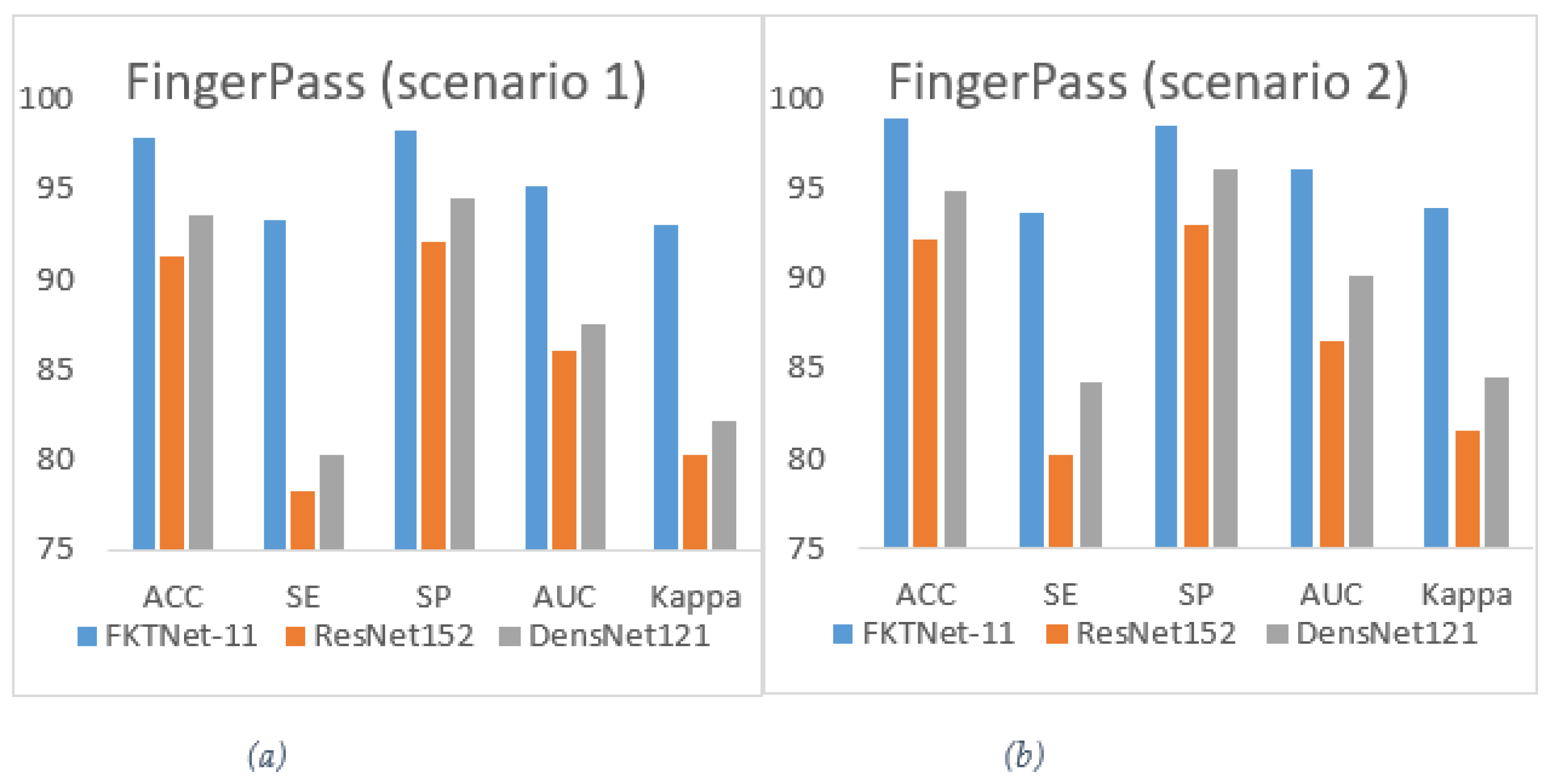
| ACC% | SE% | SP% | AUC% | Kappa% | |
| FKTNet-11 | 97.84 | 93.25 | 98.28 | 95.21 | 93.05 |
| ResNet152 | 91.22 | 78.22 | 92.05 | 86.11 | 80.32 |
| DensNet121 | 93.55 | 80.22 | 94.44 | 87.55 | 82.11 |
| (b) | |||||
| ACC% | SE% | SP% | AUC% | Kappa% | |
| FKTNet-11 | 98.9 | 93.6 | 98.5 | 96.12 | 93.93 |
| ResNet152 | 92.22 | 80.22 | 93.05 | 86.5 | 81.62 |
| DensNet121 | 94.85 | 84.22 | 96.12 | 90.21 | 84.55 |
| Model | Train ACC | Test ACC |
|---|---|---|
| Scenarios 1 | 98.65 | 97.84 |
| Scenarios 2 | 99.11 | 98.9 |
| Model | DeepFKTNet-5 | DeepFKTNet-11 | ResNet152 | DenseNet121 |
|---|---|---|---|---|
| number of params | 58.456 k | 119.599 k | 60.19 M | 7.98 M |
| FLOPs | 0.5 G | 0.9 G | 5.6 G | 1.44 G |
Publisher’s Note: MDPI stays neutral with regard to jurisdictional claims in published maps and institutional affiliations. |
© 2022 by the authors. Licensee MDPI, Basel, Switzerland. This article is an open access article distributed under the terms and conditions of the Creative Commons Attribution (CC BY) license (https://creativecommons.org/licenses/by/4.0/).
Share and Cite
Saeed, F.; Hussain, M.; Aboalsamh, H.A. Automatic Fingerprint Classification Using Deep Learning Technology (DeepFKTNet). Mathematics 2022, 10, 1285. https://doi.org/10.3390/math10081285
Saeed F, Hussain M, Aboalsamh HA. Automatic Fingerprint Classification Using Deep Learning Technology (DeepFKTNet). Mathematics. 2022; 10(8):1285. https://doi.org/10.3390/math10081285
Chicago/Turabian StyleSaeed, Fahman, Muhammad Hussain, and Hatim A. Aboalsamh. 2022. "Automatic Fingerprint Classification Using Deep Learning Technology (DeepFKTNet)" Mathematics 10, no. 8: 1285. https://doi.org/10.3390/math10081285
APA StyleSaeed, F., Hussain, M., & Aboalsamh, H. A. (2022). Automatic Fingerprint Classification Using Deep Learning Technology (DeepFKTNet). Mathematics, 10(8), 1285. https://doi.org/10.3390/math10081285