Experimental Analysis of Quantum Annealers and Hybrid Solvers Using Benchmark Optimization Problems

Abstract

This paper studies the Hamiltonian cycle problem (HCP) and the traveling salesman problem (TSP) on D-Wave quantum systems. Motivated by the fact that most libraries present their benchmark instances in terms of adjacency matrices, we develop a novel matrix formulation for the HCP and TSP Hamiltonians, which enables the seamless and automatic integration of benchmark instances in quantum platforms. We also present a thorough mathematical analysis of the precise number of constraints required to express the HCP and TSP Hamiltonians. This analysis explains quantitatively why, almost always, running incomplete graph instances requires more qubits than complete instances. It turns out that QUBO models for incomplete graphs require more quadratic constraints than complete graphs, a fact that has been corroborated by a series of experiments. Moreover, we introduce a technique for the min-max normalization for the coefficients of the TSP Hamiltonian to address the problem of invalid solutions produced by the quantum annealer, a trend often observed. Our extensive experimental tests have demonstrated that the D-Wave Advantage_system4.1 is more efficient than the Advantage_system1.1, both in terms of qubit utilization and the quality of solutions. Finally, we experimentally establish that the D-Wave hybrid solvers always provide valid solutions, without violating the given constraints, even for arbitrarily big problems up to 120 nodes.

1. Introduction

Quantum computers are the strongest contenders against conventional, silicon-based systems and gain traction by the day. Proposed by Richard Feynman in 1982, the idea of using quantum “parallelism” [1] to solve computational problems has been proven true in quite a few cases, such as Shor’s [2] and Grover’s [3] algorithms, which are more efficient than their conventional counterparts. Further information about quantum computing and quantum information is available in [4].

In the early 2000s, Kadowaki and Nishimori introduced quantum annealing, a metaheuristic based on the principles of quantum adiabatic computation [5]. Since then, it has gained prominence for tackling combinatorial optimization problems. Quantum annealing, similar to conventional simulated annealing [6], uses a multivariable function to create an energy landscape of all the possible states in a quantum superposition, with its ground state representing the problem’s solution. Then, the system goes through the quantum annealing process repeatedly until it encounters an optimal solution with a high probability. The difference between quantum and simulated annealing is the multi-qubit tunneling used by quantum annealing [5], which also improves performance due to the high degree of parallelism. Quantum annealers calculate the optimal solutions by analyzing every possible input simultaneously, an attribute that might be crucial when handling NP-complete problems. However, as of now, these methods are still in development and are mostly used as an automatic heuristic-finding program, rather than as a precise solving program [7].

Optimization problems are one of the areas where using quantum computers may prove advantageous [8,9]. To solve an optimization problem with a quantum computer, we create a Hamiltonian, the ground state of which represents an optimal solution for the problem. Using quantum annealing, a system starts in an equal superposition of all its states with said Hamiltonian applied. Over time, the system evolves according to the Schrödinger equation, and the system’s state changes depending on the strength of the local transverse field as it changes over time. To obtain the problem’s solution, we slowly turn off the transverse field, and the system settles in its ground state. If we have chosen the correct Hamiltonian, then the ground state of our system will also be its optimal solution.

D-Wave offers quantum computers that use quantum annealing for solving optimization and probabilistic sampling problems. The quantum processing units (QPUs) inside the D-Wave machines handle the quantum annealing process. The lowest energy states of the superconducting loops are the quantum bits (which we shall refer to as qubits), which are the analog of conventional bits for the QPU [10,11]. The quantum annealing process takes a system with all of its qubits in superposition and guides it towards a new state in which every qubit collapses into a value of either 0 or 1. The resulting system will be a system in a classical state, which will also be the optimal solution to the problem. In 2020, D-Wave announced their new generation of quantum computers, the Advantage System. The Advantage System uses the Pegasus topology, improving from the previous generation’s Chimera topology. The Advantage QPU contains more than 5000 qubits, with each qubit having 15 couplers to other qubits, totaling more than 35,000 couplers. Qubits in the Advantage QPU are mapped to a P16 Pegasus graph, meaning they are logically mapped into a $15\times 15\times 2$ matrix of unit cells on a diagonal grid. A Pegasus unit cell contains twenty-four qubits, with each qubit coupled to one similarly aligned qubit in the cell and two similarly aligned qubits in adjacent cells [12].

D-Wave computers excel at solving quadratic unconstrained binary optimization (QUBO for short) problems. QUBO models involve minimizing a quadratic polynomial function over binary variables [13,14], a hallmark of NP-hardness [15]. The Schrödinger equation is a linear partial differential equation. It expresses the wave function or state function of a quantum-mechanical system. By knowing the necessary variables in a system, we can model most physical systems. The Ising model is a model that is equivalent to the QUBO model. Proposed in the 1920s by Ernst Ising and Wilhelm Lenz, the Ising model is a well-researched model in ferromagnetism [16,17]. It assumes that qubits represent the model’s variables, and their interactions stand for the costs associated with each pair of qubits. The model’s design makes it possible to formulate it into an undirected graph with qubits as vertices and couplers as edges among them. In 2017, D-Wave introduced qbsolv, an open-source software that, according to D-Wave, can handle problems of arbitrary size. Qbsolv is a hybrid system, meaning it breaks down the problem’s graph into smaller subgraphs using its CPU and solves each partition using its QPU. It then repeats the process and uses a Tabu-based search to examine if a better solution is available [18].

1.1. Related Work

The Hamiltonian cycle problem (HCP for short) asks a simple yet complex-to-answer question: “Given a graph of n nodes, is there a path that passes through each node only once and returns to the starting node?” It is an NP-complete problem, first proposed in the 1850s, and a fascinating problem for computer scientists. The Flinders Hamiltonian Cycle Project (FHCP) provides benchmark graph datasets for both the HCP and TSP [19]. In this paper, we have used their small graphs, generated by GENREG [20], as they are particularly suitable for solving by the QPU without needing a hybrid solver. The traveling salesman problem (TSP from now on) is an NP-hard combinatorial optimization problem that builds upon the HCP [21]. Given a weighted graph, instead of finding the existence of a Hamiltonian cycle, the TSP seeks the cycle with the minimum total cost.

The intractable complexity of the TSP has led researchers to pursue alternative avenues. One such approach advocates for the use of metaheuristics, i.e., high-level heuristics designed to select a lower-level heuristic that can produce a fairly good solution with limited computing capacity [22]. The term “metaheuristics” was suggested by Glover. Of course, metaheuristic procedures, in contrast to exact methods, do not guarantee a global optimal solution [23]. Papalitsas et al. [24] designed a metaheuristic based on VNS for the TSP, with an emphasis on time windows. This quantum-inspired procedure was also applied successfully to the solution of real-life problems that can be modeled as TSP instances [8]. More recently, ref. [25] applied a quantum-inspired metaheuristic for tackling the practical problem of garbage collection with time windows that produced particularly promising experimental results, as further comparative analysis demonstrated in [26]. A thorough statistical and computational analysis on asymmetric, symmetric, and national TSP benchmarks from the well-known TSPLIB benchmark library was conducted in [27].

Another state-of-the-art approach for combinatorial optimization problems such as TSP is to employ unconventional computing [28,29]. It turns out that HCP and TSP are suitable candidates for a quantum annealer. An excellent reference for many Ising formulations for NP-complete and NP-hard optimization problems is the paper by Lucas [17]. In this paper, Lucas also presented the QUBO formulations for the Hamiltonian cycle problem and the traveling salesman problem, giving particular emphasis to the minimization of the usage of qubits. Another formulation of the traveling salesman problem, focusing on handling the symmetric version of the problem, was presented by Martonák et al. [30]. The basis for the QUBO formulation used in this paper was proposed by Papalitsas et al. in [31]. A recent work [32] conducted an experimental analysis of the performance of two hybrid systems provided by D-Wave, the Kerberos solver and the LeapHybridSampler solver, using the TSP as a benchmark. The conclusion of the tests in [32] is that the Kerberos solver is superior to the LHS, as Kerberos consistently yields solutions closer to the optimal route for every TSP instance. However, the LHS still produced routes that obeyed the imposed constraints for the TSP.

Contribution. Motivated by the fact that most libraries present their benchmark instances in terms of adjacency matrices, and to facilitate their execution by the quantum annealer and by tools such as qubovert [33], we set out to convert the HCP and TSP Hamiltonians in matrix form. This formulation, which we believe has not appeared previously in the literature, enables the seamless and automatic integration of the benchmark instances in quantum testing platforms. We also present a thorough mathematical analysis of the precise number of constraints required to express the HCP and TSP Hamiltonians. This analysis explains, quantitatively, why running incomplete graph instances almost always requires more qubits than complete instances. It turns out that incomplete graphs require more quadratic constraints than complete graphs. This theoretical finding has been corroborated by a series of experiments outlined in Section 5.3. Its importance is not only theoretical but practical as well since, in the current technological stage, qubits remain a precious commodity. When solving TSP instances, the solutions produced by the quantum annealer are often invalid, in the sense that they violate the topology of the graph. This is to be expected, because if the weight of an edge is higher than the constraint penalty, the annealer, to reach a lower energy state, ignores the constraint. To address this, we advocate for the use of min-max normalization of the coefficients of the TSP Hamiltonian. This well-known and easy-to-implement technique was experimentally tested and found to be considerably helpful. Furthermore, our extensive experimental tests have led us to some interesting conclusions. We discovered that D-Wave’s Advantage_system4.1 is more efficient than the older Advantage_system1.1, both in terms of qubit utilization and the quality of solutions. Using our proposed matrix formulation, it is possible to run the Burma14 instance of the TSPLIB library on a D-Wave Advantage_system4.1, although without obtaining a “correct” solution. Finally, we have established experimentally that D-Wave’s hybrid solvers always provide a valid solution to a problem and never break the constraints of a QUBO model, even for arbitrarily big problems, of the order of 120 nodes.

1.2. Organization

This paper is structured as follows. Section 2 explains the standard QUBO formulation of the HCP and TSP. Section 3 presents the matrix QUBO formulation of the HCP and TSP problems. Section 4 demonstrates the graph weight normalization procedure. Section 5 contains the experimental results obtained from our tests on D-Waves’s QPU. Section 6 presents the results from the tests conducted on D-Waves’s hybrid solver, and Section 7 summarizes and discusses the conclusions drawn from the experiments.

2. The Standard QUBO Formulation

We recall that, given a graph $G=(V,E)$, where V is the set of vertices and E is the set of edges, both HCP and TSP problems involve finding a tour:

$$\begin{array}{c}\hfill T=(p_1,\cdots ,p_n,p_{n+1}),p_{n+1}=p_1,\end{array}$$

(1)

where n is the number of vertices, and $p_i$ is the vertex in the ith position of the tour.

Typically, QUBO expressions are formed from binary decision variables, i.e., variables that can only take the values 0 or 1. In this context, these binary variables will be designated by $x_{v,p}$, and they will have the usual meaning:

$$\begin{array}{c}\hfill x_{v,p}=\left\{\begin{array}{cc}\hfill 1& \mathrm{vertex}v\mathrm{is}\mathrm{at}\mathrm{position}p\mathrm{in}\mathrm{the}\mathrm{tour},\\ \hfill 0& \mathrm{otherwise}.\hfill \end{array}\right.\end{array}$$

(2)

The HCP and TSP QUBO forms, as given by [17], are built up by the following simpler Hamiltonians:

$$\begin{array}{c}\hfill H_{v,p}=\sum _{v=1}^n{\left(1-\sum _{p=1}^n{x}_{v,p}\right)}^2\end{array}$$

(3)

$$\begin{array}{c}\hfill H_{p,v}=\sum _{p=1}^n{\left(1-\sum _{v=1}^n{x}_{v,p}\right)}^2\end{array}$$

(4)

$$\begin{array}{c}\hfill H_{E^c}=\sum _{(u,v)\notin E}^{}\sum _{p=1}^n{x}_{u,p}{x}_{v,p+1}\end{array}$$

(5)

$$\begin{array}{c}\hfill H_W=\sum _{(u,v)\in E}^{}{w}_{u,v}\sum _{p=1}^n{x}_{u,p}{x}_{v,p+1}\end{array}$$

(6)

These four Hamiltonians, $H_{v,p},H_{p,v},H_{E^c}$, and $H_W$, encode fundamental properties that capture the essence of the two problems:

• $H_{v,p}$ asserts that every vertex must appear in exactly one position of the tour;
• $H_{p,v}$ states that each position of the tour is occupied by precisely one vertex;
• $H_{E^c}$ requires that the tour is comprised of edges that “really” exist. If the tour, mistakenly, contains a “phantom” edge, i.e., an edge belonging to $E^c$, then this will incur an energy penalty;
• $H_W$ computes the cost or weight of the tour. A tour minimizing this Hamiltonian is an optimal tour.

The complete QUBO forms of the HCP and TSP problems are given below:

$$\begin{array}{c}\hfill H_{HCP}=c_1\left(H_{v,p}+H_{p,v}+H_{E^c}\right)\end{array}$$

(7)

$$\begin{array}{c}\hfill H_{TSP}=H_{HCP}+c_2{H}_W\end{array}$$

(8)

In the above formulas, $c_1$ and $c_2$ are positive constants—different, in general; we shall have more to say later about the significance of these constants. The first 3 Hamiltonians, $H_{v,p},H_{p,v}$, and $H_{E^c}$, express integrity constraints; the slightest violations render the solution invalid. The fourth Hamiltonian, $H_W$, is the minimization objective that is necessary in order to converge to the tour associated with the minimal cost.

Example 1.

To provide a clearer picture, we will give a small-scale example of formulating a TSP into QUBO, using the graph $G_1$ shown in Figure 1. The problem’s graph has $n=4$ nodes, and its adjacency matrix is given by (9). Using Equations (3)–(8), we can construct the Hamiltonian of the QUBO model for solving the TSP in this graph, as shown below. To emphasize the fact the Hamiltonians computed in this example refer to the particular graph $G_1$, we use the notations $H_{v,p}^{G_1}$, $H_{p,v}^{G_1}$, $H_{E^c}^{G_1}$, $H_W^{G_1}$, $H_{HCP}^{G_1}$, and $H_{TSP}^{G_1}$ when referring to them.

$$\begin{array}{c}\hfill W=\left[\begin{array}{cccc}\hfill 0\hfill & \hfill 30\hfill & \hfill 42\hfill & 12\\ \hfill 30\hfill & \hfill 0\hfill & \hfill 20\hfill & 34\\ \hfill 42\hfill & \hfill 20\hfill & \hfill 0\hfill & 35\\ \hfill 12\hfill & \hfill 34\hfill & \hfill 35\hfill & 0\end{array}\right]\hfill \end{array}$$

(9)

Now, the general expression ${\left(1-{\sum }_{p=1}^n{x}_{v,p}\right)}^2$ reduces to ${\left(1-x_{v,1}-x_{v,2}-x_{v,3}-x_{v,4}\right)}^2$. This expression can be further simplified by taking into account the identity:

$$\begin{array}{cc}\hfill & {(1-a-b-c-d)}^2\hfill \\ \hfill & =1+a^2+b^2+c^2+d^2-2a-2b-2c-2d+2ab+2ac+2ad+2bc+2bd+2cd,\hfill \end{array}$$

(10)

and the fact that the square of a binary decision variable is just the variable:

$$\begin{array}{c}\hfill x_{v,p}^2=x_{v,p},\end{array}$$

(11)

to give:

$$\begin{array}{cc}\hfill {\left(1-\sum _{p=1}^4{x}_{v,p}\right)}^2& ={\left(1-x_{v,1}-x_{v,2}-x_{v,3}-x_{v,4}\right)}^2\hfill \\ \hfill & =1+x_{v,1}+x_{v,2}+x_{v,3}+x_{v,4}-2x_{v,1}-2x_{v,2}-2x_{v,3}-2x_{v,4}\hfill \\ \hfill & +2x_{v,1}{x}_{v,2}+2x_{v,1}{x}_{v,3}+2x_{v,1}{x}_{v,4}+2x_{v,2}{x}_{v,3}+2x_{v,2}{x}_{v,4}+2x_{v,3}{x}_{v,4}\hfill \\ \hfill & =1-x_{v,1}-x_{v,2}-x_{v,3}-x_{v,4}\hfill \\ \hfill & +2x_{v,1}{x}_{v,2}+2x_{v,1}{x}_{v,3}+2x_{v,1}{x}_{v,4}+2x_{v,2}{x}_{v,3}+2x_{v,2}{x}_{v,4}+2x_{v,3}{x}_{v,4}.\hfill \end{array}$$

(12)

Therefore:

$$\begin{array}{c}\hfill H_{v,p}^{G_1}=\sum _{v=1}^4{\left(1-\sum _{p=1}^4{x}_{v,p}\right)}^2\\ \hfill =4-x_{1,1}-x_{1,2}-x_{1,3}-x_{1,4}-x_{2,1}-x_{2,2}-x_{2,3}-x_{2,4}\\ \hfill -x_{3,1}-x_{3,2}-x_{3,3}-x_{3,4}-x_{4,1}-x_{4,2}-x_{4,3}-x_{4,4}\\ \hfill +2x_{1,1}{x}_{1,2}+2x_{1,1}{x}_{1,3}+2x_{1,1}{x}_{1,4}+2x_{1,2}{x}_{1,3}+2x_{1,2}{x}_{1,4}+2x_{1,3}{x}_{1,4}\\ \hfill +2x_{2,1}{x}_{2,2}+2x_{2,1}{x}_{2,3}+2x_{2,1}{x}_{2,4}+2x_{2,2}{x}_{2,3}+2x_{2,2}{x}_{2,4}+2x_{2,3}{x}_{2,4}\\ \hfill +2x_{3,1}{x}_{3,2}+2x_{3,1}{x}_{3,3}+2x_{3,1}{x}_{3,4}+2x_{3,2}{x}_{3,3}+2x_{3,2}{x}_{3,4}+2x_{3,3}{x}_{3,4}\\ \hfill +2x_{4,1}{x}_{4,2}+2x_{4,1}{x}_{4,3}+2x_{4,1}{x}_{4,4}+2x_{4,2}{x}_{4,3}+2x_{4,2}{x}_{4,4}+2x_{4,3}{x}_{4,4}.\end{array}$$

(13)

In a similar way, we may construct $H_{p,v}^{G_1}$:

$$\begin{array}{c}\hfill H_{p,v}^{G_1}=\sum _{p=1}^4{\left(1-\sum _{v=1}^4{x}_{v,p}\right)}^2\\ \hfill =4-x_{1,1}-x_{2,1}-x_{3,1}-x_{4,1}-x_{1,2}-x_{2,2}-x_{3,2}-x_{4,2}\\ \hfill -x_{1,3}-x_{2,3}-x_{3,3}-x_{4,3}-x_{1,4}-x_{2,4}-x_{3,4}-x_{4,4}\\ \hfill +2x_{1,1}{x}_{2,1}+2x_{1,1}{x}_{3,1}+2x_{1,1}{x}_{4,1}+2x_{2,1}{x}_{3,1}+2x_{2,1}{x}_{4,1}+2x_{3,1}{x}_{4,1}\\ \hfill +2x_{1,2}{x}_{2,2}+2x_{1,2}{x}_{3,2}+2x_{1,2}{x}_{4,2}+2x_{2,2}{x}_{3,2}+2x_{2,2}{x}_{4,2}+2x_{3,2}{x}_{4,2}\\ \hfill +2x_{1,3}{x}_{2,3}+2x_{1,3}{x}_{3,3}+2x_{1,3}{x}_{4,3}+2x_{2,3}{x}_{3,3}+2x_{2,3}{x}_{4,3}+2x_{3,3}{x}_{4,3}\\ \hfill +2x_{1,4}{x}_{2,4}+2x_{1,4}{x}_{3,4}+2x_{1,4}{x}_{4,4}+2x_{2,4}{x}_{3,4}+2x_{2,4}{x}_{4,4}+2x_{3,4}{x}_{4,4}.\end{array}$$

(14)

Each of the expansions of $H_{v,p}^{G_1}$ and $H_{p,v}^{G_1}$, as given in (13) and (14), create a constant term, namely, 4, and 40 constraints in total: 16 linear constraints and 24 quadratic constraints. The linear constraints are the same, but the quadratic constraints are different.

$H_{E^c}$ depends on the topology of the graph. In our example, where the graph is complete, $H_{E^c}^{G_1}$ would only involve self-loops, that is:

$$\begin{array}{c}\hfill H_{E^c}^{G_1}=\sum _{(u,v)\notin E}^{}\sum _{p=1}^4{x}_{u,p}{x}_{v,p+1}\\ \hfill =x_{1,1}{x}_{1,2}+x_{1,2}{x}_{1,3}+x_{1,3}{x}_{1,4}+x_{1,4}{x}_{1,1}+x_{2,1}{x}_{2,2}+x_{2,2}{x}_{2,3}+x_{2,3}{x}_{2,4}+x_{2,4}{x}_{2,1}\\ \hfill +x_{3,1}{x}_{3,2}+x_{3,2}{x}_{3,3}+x_{3,3}{x}_{3,4}+x_{3,4}{x}_{3,1}+x_{4,1}{x}_{4,2}+x_{4,2}{x}_{4,3}+x_{4,3}{x}_{4,4}+x_{4,4}{x}_{4,1}.\end{array}$$

(15)

To avoid any potential confusion, let us point out that, in the tour, which is a cycle, position $n+1$ coincides with position 1, a fact which was used in the formulation of (15). As a result of the completeness of the graph, all of the above 16 quadratic constraints are already present in $H_{v,p}^{G_1}$, as can be verified by recalling (13). Of course, their presence in $H_{E^c}^{G_1}$ increases by 1 their corresponding coefficient, amplifying their relative significance. It is useful to briefly consider what happens when the graph is not complete, i.e., when at least one edge that is not a self-loop is missing. If, for instance, $G=(V,E)$ is an undirected graph and $(1,3)\notin E$, which implies that also $(3,1)\notin E$, then $H_{E^c}^{G_1}$, apart from the constraints shown in (15), would additionally contain the following constraints:

$$\begin{array}{c}\hfill x_{1,1}{x}_{3,2}+x_{1,2}{x}_{3,3}+x_{1,3}{x}_{3,4}+x_{1,4}{x}_{3,1}+x_{3,1}{x}_{1,2}+x_{3,2}{x}_{1,3}+x_{3,3}{x}_{1,4}+x_{3,4}{x}_{1,1}.\end{array}$$

(16)

If, on the other hand, $G=(V,E)$ is a directed graph and $(1,3)\notin E$, which does not necessarily imply that $(3,1)\notin E$, then $H_{E^c}^{G_1}$, apart from the constraints shown in (15), would additionally contain the following constraints:

$$\begin{array}{c}\hfill x_{1,1}{x}_{3,2}+x_{1,2}{x}_{3,3}+x_{1,3}{x}_{3,4}+x_{1,4}{x}_{3,1}.\end{array}$$

(17)

$H_W$ captures the topology of the graph and the cost, also referred to as the weight, associated with each edge. In this particular example, it will produce the constraints listed below, where we have again identified position $n+1$ with position 1:

$$\begin{array}{cc}\hfill H_W^{G_1}& =\sum _{(u,v)\in E}^{}{w}_{u,v}\sum _{p=1}^4{x}_{u,p}{x}_{v,p+1}\hfill \\ \hfill & =30x_{1,1}{x}_{2,2}+30x_{1,2}{x}_{2,3}+30x_{1,3}{x}_{2,4}+30x_{1,4}{x}_{2,1}+42x_{1,1}{x}_{3,2}+42x_{1,2}{x}_{3,3}+42x_{1,3}{x}_{3,4}+42x_{1,4}{x}_{3,1}\hfill \\ \hfill & +12x_{1,1}{x}_{4,2}+12x_{1,2}{x}_{4,3}+12x_{1,3}{x}_{4,4}+12x_{1,4}{x}_{4,1}+30x_{2,1}{x}_{1,2}+30x_{2,2}{x}_{1,3}+30x_{2,3}{x}_{1,4}+30x_{2,4}{x}_{1,1}\hfill \\ \hfill & +20x_{2,1}{x}_{3,2}+20x_{2,2}{x}_{3,3}+20x_{2,3}{x}_{3,4}+20x_{2,4}{x}_{3,1}+34x_{2,1}{x}_{4,2}+34x_{2,2}{x}_{4,3}+34x_{2,3}{x}_{4,4}+34x_{2,4}{x}_{4,1}\hfill \\ \hfill & +42x_{3,1}{x}_{1,2}+42x_{3,2}{x}_{1,3}+42x_{3,3}{x}_{1,4}+42x_{3,4}{x}_{1,1}+20x_{3,1}{x}_{2,2}+20x_{3,2}{x}_{2,3}+20x_{3,3}{x}_{2,4}+20x_{3,4}{x}_{2,1}\hfill \\ \hfill & +35x_{3,1}{x}_{4,2}+35x_{3,2}{x}_{4,3}+35x_{3,3}{x}_{4,4}+35x_{3,4}{x}_{4,1}+12x_{4,1}{x}_{1,2}+12x_{4,2}{x}_{1,3}+12x_{4,3}{x}_{1,4}+12x_{4,4}{x}_{1,1}\hfill \\ \hfill & +34x_{4,1}{x}_{2,2}+34x_{4,2}{x}_{2,3}+34x_{4,3}{x}_{2,4}+34x_{4,4}{x}_{2,1}+35x_{4,1}{x}_{3,2}+35x_{4,2}{x}_{3,3}+35x_{4,3}{x}_{3,4}+35x_{4,4}{x}_{3,1}.\hfill \end{array}$$

(18)

The expansion of $H_W^{G_1}$, shown in (18), creates 48 new quadratic constraints. It is instructive to see what changes if the graph is not complete, assuming, as before, that the missing edges are not self-loops. If the are m edges present, then each such edge will involve n (here $n=4$) quadratic constraints.

In view of (7), the HCP Hamiltonian for $G_1$ is $H_{HCP}^{G_1}$=$c_1$$\left(H_{v,p}^{G_1}+H_{p,v}^{G_1}+H_{E^c}^{G_1}\right)$, where $c_1$ is a positive constant. $H_{HCP}^{G_1}$ is constructed by combining (13) and (14); it requires 16 binary variables, and it involves 64 constraints. Analogously, the Hamiltonian for solving the TSP on $G_1$ is $H_{TSP}^{G_1}=H_{HCP}^{G_1}+c_2{H}_W^{G_1}$, where $c_2$ is also a positive constant. Since $H_{TSP}^{G_1}$ is constructed by combining (13), (14), and (18), it contains 112 constraints.

Using the previous example as a starting point, it is straightforward to derive the number of constraints for a general graph with n nodes. In the QUBO formulation, the binary variables corresponding to an edge (or arc) $(u,v)$ are distinct from the binary variables corresponding to the edge (or arc) $(v,u)$. Therefore, they give rise to distinct constraints in the Hamiltonians $H_{HCP}$ and $H_{TSP}$. Hence, from this perspective, irrespective of whether a complete graph $G=(V,E)$ with n nodes is directed or undirected, it should be considered as having $n(n-1)$ edges. In other words, even in an undirected graph, we should view the edges $(u,v)$ and $(v,u)$ as different.

• The Hamiltonians $H_{v,p}$ and $H_{p,v}$, as given in (13) and (14), require a constant term, namely, n, $n^2$ linear constraints, and $\frac{n^2(n-1)}{2}$ quadratic constraints, which brings the total number of constraints to $\frac{n^2(n+1)}{2}$. The linear constraints are the same in both $H_{v,p}$ and $H_{p,v}$, but the quadratic constraints are different;
• If the graph is complete, then $H_{E^c}$ does not add any new constraints. To be precise, $H_{E^c}$ involves $n^2$ quadratic constraints, which are also present in the $H_{v,p}$ Hamiltonian. Hence, $H_{E^c}$ only enhances the relative weight of existing constraints;
• If the graph is not complete, then $H_{E^c}$ creates, for each missing edge $(u,v)\notin E$ that is not a self-loop, i.e., $u\ne v$, n additional constraints. If k such edges are missing, there will be $nk$ additional quadratic constraints in total. This fact is experimentally validated from the results presented in Section 5.3;
• In a complete graph with n nodes, $H_W$ introduces $n^2(n-1)=n\left|E\right|$ quadratic constraints, where $\left|E\right|$ stands for the number of edges in the graph. This formula can be generalized further to the case where the graph is not complete and has m edges. In such a case, $H_W$ will add $nm$ quadratic constraints.

• In a complete graph, $H_{HCP}$ requires $n^2$ binary variables and $n^3$ constraints in total (recall that the $n^2$ linear constraints are the same). If the graph is not complete, it requires more constraints: specifically, $n^3+nk$, where k is the number of missing edges;
• For a complete graph, $H_{TSP}$ requires $n^2$ binary variables, $2n^2(n-1)=2n\left|E\right|$ quadratic constraints, and $n^2(2n-1)$ constraints in total. If the graph is not complete, it requires $n^3+n(m+k)$, where m is the number of existing edges and k is the number of missing edges;
• In the typical and practically important case where we have a simple graph, that is, a graph with no self-loops and no parallel edges, then $m+k=n(n-1)$. The previous formulas now give $2n^2(n-1)$ quadratic constraints and $n^2(2n-1)$ total constraints. In this case, the number of constraints required for the $H_{TSP}$ Hamiltonian is equal to the number of constraints required when the graph is complete.

Table 1. This table summarizes the number of constraints that are involved in each of the Hamiltonians (3)–(8), when applied to a complete graph with n nodes.

Number of Binary Variables: $n^2$
	Number of Constraints
Hamiltonian	Linear	Quadratic	Total
$H_{v,p}$	$n^2$	$\frac{n^2(n-1)}{2}=n\left|E\right|$	$\frac{n^2(n+1)}{2}$
$H_{p,v}$	$n^2$	$\frac{n^2(n-1)}{2}=n\left|E\right|$	$\frac{n^2(n+1)}{2}$
$H_{E^c}$	0	0	0
$H_W$	0	$n^2(n-1)=n\left|E\right|$	$n^2(n-1)=n\left|E\right|$
$H_{HCP}$	$n^2$	$n^2(n-1)$	$n^3$
$H_{TSP}$	$n^2$	$2n^2(n-1)=2n\left|E\right|$	$n^2(2n-1)$

,

Table 2. This table summarizes the number of constraints that are involved in each of the Hamiltonians (3)–(8), when applied to an arbitrary graph with n nodes, m edges, and k missing edges (none of which are a self-loop).

Number of Binary Variables: $n^2$
	Number of Constraints
Hamiltonian	Linear	Quadratic	Total
$H_{v,p}$	$n^2$	$\frac{n^2(n-1)}{2}$	$\frac{n^2(n+1)}{2}$
$H_{p,v}$	$n^2$	$\frac{n^2(n-1)}{2}$	$\frac{n^2(n+1)}{2}$
$H_{E^c}$	0	$nk$	$nk$
$H_W$	0	$nm$	$nm$
$H_{HCP}$	$n^2$	$n^2(n-1)+nk$	$n^3+nk$
$H_{TSP}$	$n^2$	$n^2(n-1)+n(m+k)$	$n^3+n(m+k)$

and

Table 3. This table shows the number of constraints that are involved in the $H_{TSP}$ Hamiltonian (8), when $m+k=n(n-1)$.

Number of Constraints when $m+k=n(n-1)$
Hamiltonian	Linear	Quadratic	Total
$H_{TSP}$	$n^2$	$2n^2(n-1)=2n\left|E\right|$	$n^2(2n-1)$

summarize the above observations regarding the number of constraints involved in the HCP and TSP Hamiltonians.

3. The Matrix QUBO Formulation

In this section, we shall present the matrix form of the Hamiltonians (3)–(8), so as to enable their seamless execution of HCP and TSP instances by the quantum annealer and by tools such as qubovert [33]. For this purpose, we define, for each $v\in V$, the column vector $X_v$ containing the binary decision variables $x_{v,1},x_{v,2},\cdots ,x_{v,n}$ corresponding to the possible positions of vertex v in the tour. Then, by combining the n vectors $X_v,1\le v\le n$, we construct the column vector X, which of course has $n^2$ rows:

(19)

(20)

The matrices appropriate for expressing (7) and (8) must be built from simpler matrices that capture the Hamiltonians (3)–(6). To define the latter in the easiest way, we need a few auxiliary $n\times n$ matrices. The $n\times n$ identity matrix is denoted by $I_n$, and its negation by $-I_n$. The $n\times n$ zero matrix whose entries are all 0 is denoted by $O_n$. Another special-form $n\times n$ matrix, particularly designed for $H_{v,p}$, is designated by $J_n$:

(21)

(22)

(23)

(24)

In order to capture the effect of the weight of each existing edge on the Hamiltonians, as well as the effect of each missing edge, we make use of two more auxiliary special-form $n\times n$ matrices: $L_{v,v}$, designed specifically to tackle self-loops, i.e., edges of the form $(v,v)$; and $L_{u,v}$, with $u\ne v$, designed for edges that are not self-loops:

(25)

(26)

Let us assume that $W=\left[w_{u,v}\right]$ is the $n\times n$ adjacency matrix characterizing the topology of the given graph. In this matrix, if $w_{u,v}=0$, then the edge (or arc) $(u,v)$ does not exist in the graph, whereas if $w_{u,v}>0$, then $w_{u,v}$ expresses the cost or weight associated with $(u,v)$. To each entry $w_{u,v}$ of W, we associate two $n\times n$ matrices, $W_{(u,v)}$ and $W_{\overline{(u,v)}}$, defined as follows:

$$\begin{array}{c}\hfill W_{(u,v)}=w_{u,v}{L}_{u,v}\end{array}$$

(27)

$$\begin{array}{c}\hfill W_{\overline{(u,v)}}=\left\{\begin{array}{cc}\hfill L_{u,v}& \mathrm{if}{w}_{u,v}=0,\\ \hfill O_n& \mathrm{if}{w}_{u,v}>0.\end{array}\right.\end{array}$$

(28)

We proceed now to give the matrix form of the Hamiltonians (3)–(6). Specifically, we establish the correspondence between the Hamiltonians and $n^2\times n^2$ block matrices shown below, where the symbol ↦ is used to convey association and not equality:

(29)

(30)

(31)

(32)

In view of the relations (29)–(32), the sum of the three Hamiltonians $H_{v,p}+H_{p,v}+H_{E^c}$ can be associated with the linear expression $2n+X^{\top }\left(M_{v,p}+M_{p,v}+M_{E^c}\right)X$, where X is the column vector of the binary variables given by (20). The constant term $2n$ is irrelevant in the whole quantum annealing process, and can be omitted. By defining, for succinctness, the matrix $M_{HCP}$, the Hamiltonian $H_{HCP}$ can be expressed in matrix form, as shown below:

$$\begin{array}{c}\hfill H_{HCP}=X^{\top }{M}_{HCP}X\end{array}$$

(33)

$$\begin{array}{c}\hfill M_{HCP}=c_1\left(M_{v,p}+M_{p,v}+M_{E^c}\right)\end{array}$$

(34)

Analogously, $H_{TSP}$ can be cast in a compact matrix form with the help of the auxiliary matrix $M_{TSP}$:

$$\begin{array}{c}\hfill H_{HCP}=X^{\top }{M}_{TSP}X\end{array}$$

(35)

$$\begin{array}{c}\hfill M_{TSP}=M_{HCP}+c_2{M}_W\end{array}$$

(36)

Example 2.

To demonstrate how the previous machinery can be utilized, we return to the graph $G_1$ of Example 1, and express the HCP and TSP Hamiltonians as matrices. For clarity of presentation and simplicity, we will take the two positive constants, $c_1$ and $c_2$, equal to 1. To emphasize the fact the X and the matrices computed in this example refer to the particular graph $G_1$, we use the notations $X^{G_1}$, $M_{v,p}^{G_1}$, $M_{p,v}^{G_1}$, $M_{E^c}^{G_1}$, $M_W^{G_1}$, $M_{HCP}^{G_1}$, and $M_{TSP}^{G_1}$ when referring to them. In this example, the column vector $X^{G_1}$, containing the $n^2=16$ binary variables, is listed below. Note that, in order to save space, we actually show ${\left(X^{G_1}\right)}^{\top }$:

$$\begin{array}{cc}\hfill {\left(X^{G_1}\right)}^{\top }& =\left[\begin{array}{cccccccc}\hfill x_{1,1}& \hfill x_{1,2}& \hfill x_{1,3}& x_{1,4}& x_{2,1}& x_{2,2}& x_{2,3}& x_{2,4}\end{array}\right]\hfill \\ \hfill & \left[\begin{array}{cccccccc}\hfill x_{3,1}& \hfill x_{3,2}& \hfill x_{3,3}& x_{3,4}& x_{4,1}& x_{4,2}& x_{4,3}& x_{4,4}\end{array}\right]\hfill \end{array}$$

(37)

Matrices $M_{v,p}^{G_1},M_{p,v}^{G_1},M_{E^c}^{G_1}$, and $M_W^{G_1}$, adopted to the specific graph $G_1$, now become as follows:

(38)

(39)

(40)

A straightforward computation of the expressions $X^{\top }{M}_{v,p}^{G_1}X$ and $X^{\top }{M}_{p,v}^{G_1}X$ produces exactly the same constraints (minus the constant terms) as those given by Equations (13) and (14). $M_{v,p}^{G_1}$ and $M_{p,v}^{G_1}$ are generic, in the sense that they do not convey any specific information about the graph at hand. The topology of the graph is captured by $M_{E^c}^{G_1}$ and $M_W^{G_1}$. Since $G_1$ is complete, matrix $M_{E^c}^{G_1}$ assumes a particularly simple form. As expected, by explicitly computing $X^{\top }{M}_{E^c}^{G_1}X$, we obtain exactly the same 16 constraints encountered in (15). For completeness, we show the form of the matrix $M_{E^c}^{G_1}$ when $(1,3)\notin E$, which also implies that $(3,1)\notin E$:

(41)

By explicitly computing $X^{\top }{M}_{E^c}^{G_1}X$, we obtain, apart from the 16 constraints encountered in (15), the 8 additional quadratic constraints given by (16). By combining the matrices $M_{v,p}^{G_1},M_{p,v}^{G_1}$, and $M_{E^c}^{G_1}$, as given by (38)–(40), respectively, according to Equations (33) and (34), where, as explained before, constant $c_1=1$ for simplicity, we derive the matrix $M_{HCP}^{G_1}$ and the matrix form of the Hamiltonian $H_{HCP}^{G_1}$:

(42)

$$\begin{array}{c}\hfill H_{HCP}^{G_1}=X^{\top }{M}_{HCP}^{G_1}X\end{array}$$

(43)

(44)

The quantitative information contained in the adjacency matrix (9), which gives the topology of the graph and the weight of each edge, is incorporated in the $M_W^{G_1}$ matrix. $X^{\top }{M}_W^{G_1}X$ creates the same 48 constraints as those given by (18). By adding the matrices $M_{HCP}^{G_1}$ and $M_W^{G_1}$, as per (36), and taking $c_2=1$ for simplicity, we derive $M_{TSP}^{G_1}$ and the matrix form of the Hamiltonian $H_{TSP}^{G_1}$:

(45)

$$\begin{array}{c}\hfill H_{TSP}^{G_1}=X^{\top }{M}_{TSP}^{G_1}X\end{array}$$

(46)

This small-scale example was successfully tested on D-Wave’s Advantage_System4.1, which produced the optimal tour $T^{OPT}=(1,2,3,4)$ with optimal cost (97). Incidentally, the “incomplete” version, where edges $(1,3)$ and $(3,1)$ are missing, was also successfully solved, yielding the same optimal path and the same optimal cost.

4. Normalizing Graph Weights

During the extensive experimental tests of various instances of the TSP, a certain pattern consistently emerged. The aforementioned pattern demonstrates emphatically the importance of the numerical values of the weights used in the TSP Hamiltonian. In almost every occasion where the weights of the graph were above a certain threshold, e.g., 10, the annealer preferred to break one or more of the imposed validity constraints rather than strictly adhere to the topology of the graph. In hindsight, one could say that this is indeed the rational and expected behavior. If the weight of an edge is higher than the constraint penalty, the annealer, in order to reach a lower energy state, ignores the constraint, thus converging to solutions that violate the topology of the graph. On the bright side, the predictability of this behavior gives us the opportunity to remedy this problem. The solution that worked best in our experimental tests was the min-max normalization [34] applied to the weights of the matrix $M_W$ before adding the constraints. After the normalization process, the weight values are still proportional but lower than the constraint penalties.

Specifically, given the $n^2\times n^2$ matrix $M_W=\left[m_{i,j}\right]$, we denote by $m_{min}$ and $m_{max}$ the minimal and maximal elements of $M_W$, where, without loss of generality, we assume that $m_{min}\ne m_{max}$. All elements of $M_W$ are modified according to Equation (49), and the resulting normalized matrix is designated by $N_W$. Therefore, by defining appropriately the normalized matrix $N_{TSP}$, encompassing all the normalized constraints, we derive the normalized matrix form of the Hamiltonian $H_{TSP}$, as shown below. From now on, without further mention, we shall always employ this normalized matrix:

$$\begin{array}{c}\hfill N_{TSP}=M_{HCP}+N_W\end{array}$$

(47)

$$\begin{array}{c}\hfill H_{HCP}=X^{\top }{N}_{TSP}X\end{array}$$

(48)

Example 3.

We explain the normalization process by examining how it can be applied to the matrix $M_W^{G_1}$, as given by (44). Attempting to solve the TSP using $H_{TSP}^{G_1}$ given by Equation (46), which is based on the $M_{TSP}^{G_1}$ matrix of Equation (45), will typically yield a solution that violates some integrity constraints. We can counteract this by applying the normalization Algorithm 1. The final normalized QUBO model is shown below:

$$\begin{array}{c}\hfill N_W[i,j]=\frac{M_W[i,j]-m_{min}}{m_{max}-m_{min}}\end{array}$$

(49)

Algorithm 1: Min-max normalization.

(50)

After the normalization, the constraints imposed on the QUBO model by the weights of the TSP graph retain their respective importance, while assuming a range from 0 (for the minimum weight) to 1 (for the maximum weight). Thus, we can impose the rest of our constraints without conflicts, as the higher values in the previous QUBO model no longer overshadow them, forcing the annealer to ignore them.

Figure 2 demonstrates the importance of the normalization process as a tool that amplifies the probability that the solutions produced by the annealer will not violate any of the constraints imposed by the QUBO model. To test its effectiveness, we ran a total of 20 experiments on D-Wave’s LeapHybridSampler. The normalization procedure was applied to exactly half of the instances, e.g., 10, and the other instances were executed without normalization. As shown in Figure 2, LeapHybridSampler failed to yield a solution satisfying the graph topology in all 10 instances that were not normalized, whereas LeapHybridSampler succeeded in producing a valid solution in all 10 normalized instances.

5. Experimenting on D-Wave’s QPU

Our experiments were conducted on two of D-Wave’s available QPUs—in particular, on the Advantage_System1.1 [35], which has been decommissioned since late-2021 [36]), and on the newer version, Advantage_System4.1 [37].

5.1. HCP Using QPU

As explained in Section 1, the Hamiltonian cycle problem (HCP) is the basis for the traveling salesman problem (TSP), and its solution is an integral part of the solution for the TSP. We solved the HCP using both QPU systems available from D-Wave, namely, the Advantage_system1.1 and Advantage_system4.1. The Flinders Hamiltonian Cycle Project (FHCP) provides many benchmarking graph datasets for both the HCP and the TSP [19]. We used their dataset of small graphs, namely, the graph instances H_6, H_8, H_10, H_12, and H_14, generated by GENREG [20]. Their small number of nodes made them fit to run on the D-Wave Quantum Annealer’s available qubits without requiring the use of a hybrid solver. The average metrics that were obtained during the experiments are summarized in

Table 4. This table contains the average metrics obtained from solving HCP instances using D-Wave’s QPU.

Nodes	Solver	Runs	QAT (μs)	Qubits	Success Rate (%)
6	Advantage_system1.1	20	126,643.89	126.83	100.0
6	Advantage_system4.1	20	140,461.42	120.27	100.0
8	Advantage_system1.1	20	147,772.21	388.25	15.0
8	Advantage_system4.1	20	160,148.34	372.60	35.0
10	Advantage_system1.1	20	168,190.20	1010.20	0.0
10	Advantage_system4.1	20	209,123.62	910.15	0.0
12	Advantage_system1.1	20	170,374.85	2091.70	0.0
12	Advantage_system4.1	20	243,015.98	1924.95	0.0
14	Advantage_system1.1	20	188,910.52	3913.45	0.0
14	Advantage_system4.1	20	272,583.67	3413.00	0.0

. The “Nodes” column contains the number of nodes of the graphs, the “Solver” column shows the selected QPU that was used to solve the problem, and the “Runs” column gives the total number of times the experiment was executed. The “QAT” column shows the QPU access time, that is, the average time the quantum processing unit took to solve the problem over all runs. The “Qubits” column contains the average number of qubits used in the embedding for each run. Finally, the “Success Rate” column depicts the percentage of runs that provided a solution that did not violate any of the imposed constraints.

As can be seen, violations of the imposed constraints start to appear when the number of nodes $n\ge 8$. This is in line with similar findings in a recent work [38]. We point out the clear improvements of the Advantage_system4.1 compared to the Advantage_system1.1, both with respect to the success rate and the qubit usage. While the Advantage_system4.1 seems to be relatively slower, it more than makes up for it by offering better overall performance.

Figure 3 gives the average number of qubits used in the embedding as a function of the number of nodes per graph. This visualization shows the graphs for the Advantage_system1.1 solver, the Advantage_system4.1, and the expected qubits per instance. The ”Expected” line in the graph indicates the number of qubits the solver is expected to use, based on the constraints created in Table 2, for each of the graphs used in the experiments. Both the Advantage_system1.1 and the Advantage_system4.1 demonstrate a rapidly increasing growth in the number of qubits as n increases. One can also see that, near and after the intersection points between the solvers’ lines and the expected qubits’ line, is the point where the QPU starts breaking the imposed constraints. It is also noteworthy that the intersection point of the Advantage_system4.1 is to the right of the Advantage_system1.1, something that reflects the first solver’s superior success rate.

Figure 4 provides a comparison of the average QPU access time between the two solvers. It is evident that the Advantage_system4.1 needs more time to solve the problems, even if the difference is minuscule for real-world metrics. However, this relative loss of speed is compensated for by the decrease in qubits in the embedding, meaning that the Advantage_system4.1 can handle bigger instances in a more satisfactory way.

5.2. TSP Using QPU

Moving from the HCP to the TSP is, in principle, quite straightforward, as their main difference is the introduction of weights on the graph. In our experiments, we relied on the TSPLIB. The TSPLIB is a library of TSP graph instances, commonly used for benchmarking algorithms that aim to solve the TSP [39]. The TSPLIB instance with the least number of nodes is the burma14 graph, with just $n=14$ nodes.

Table 5. This table contains the average metrics obtained from solving TSP instances using D-Wave’s QPU.

Nodes	Solver	Runs	QAT (μs)	Qubits	Cost	Success Rate (%)
14	Advantage_system4.1	20	282,016.86	4145.25	4737.70	0.0

below contains the average metrics that were gathered during the experiments. The “Nodes” column contains the number of nodes of the graphs, the “Solver” column shows the selected QPU that was used to solve the problem, and the “Runs” column gives the total number of times the experiment was executed. The “QAT” column shows the QPU access time, that is, the average time the quantum processing unit took to solve the problem over all runs. The “Qubits” column contains the average number of qubits used in the embedding for each run. The “Cost” column shows the average cost of the solution path for each run. Finally, the “Success Rate” column depicts the percentage of runs that provided a solution that did not violate any of the imposed constraints.

The results in Table 5 are quite similar to those obtained in the HCP case. Every run produced a solution that violated at least one of the integrity constraints. The qubit usage on the Advantage_system4.1 is visually depicted in Figure 5. The number of qubits used is slightly higher than the optimal number given in Table 1 of Section 2. This, coupled with the improvement of the results produced by the Advantage_system4.1 shown in Table 4, is a clear indicator of the degree of technological progress achieved.

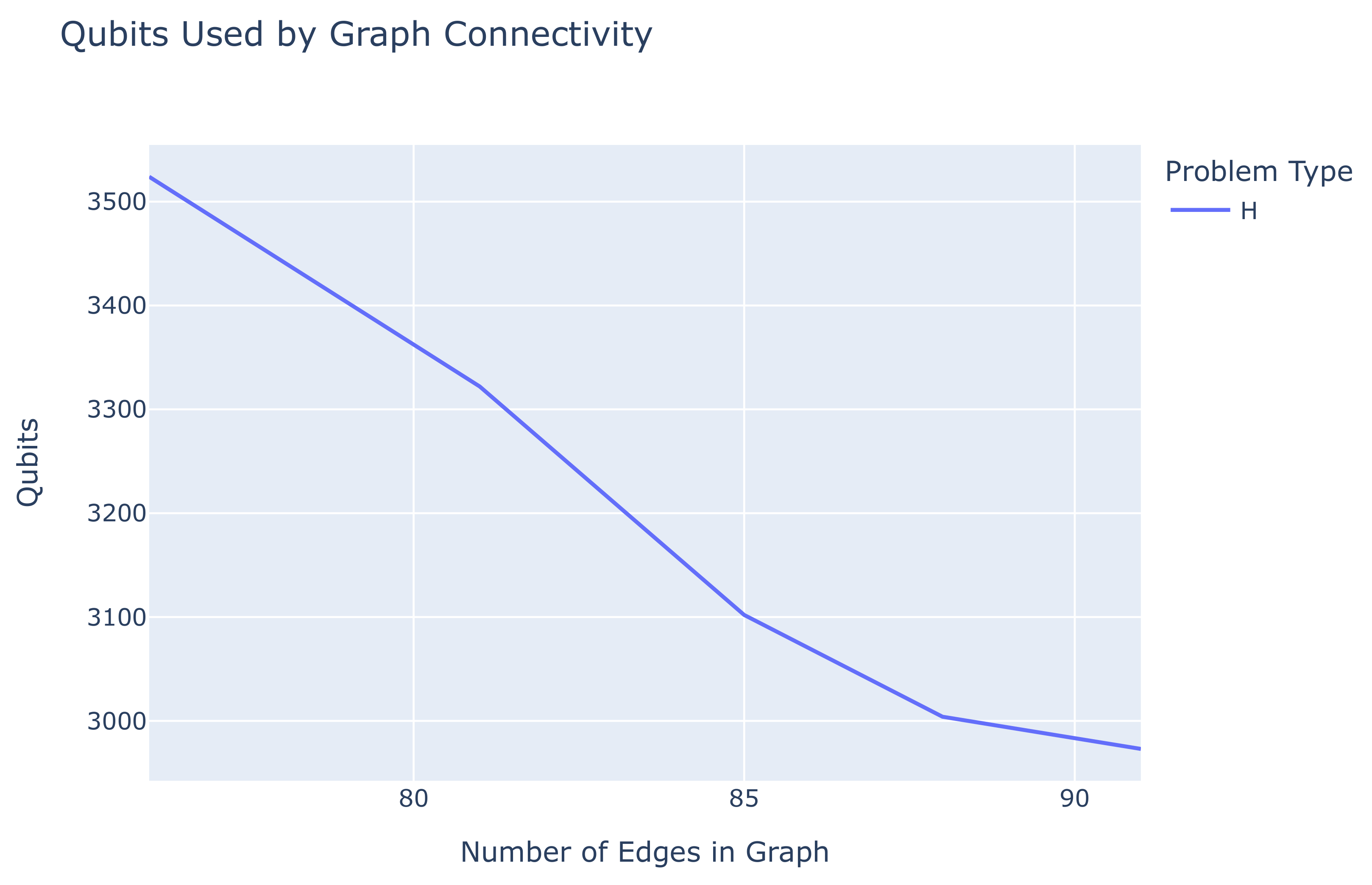
5.3. The Effect of Graph Connectivity on Qubit Usage

When comparing the results from the experiments, a consistent pattern emerged. Solving the HCP on graphs that were not complete, i.e., that were “missing” edges, always required more qubits than solving the HCP on complete graphs with the same number of nodes. We believe that this fact is the experimental validation of the theoretical results derived in Example 1 and quantified in Table 1, Table 2 and Table 3, which stipulate that, when solving the HCP, incomplete graphs require more integrity constraints than complete graphs. In particular, the HCP on a graph with n nodes and k missing edges requires $nk$ additional quadratic constraints, compared to a complete graph with n nodes. To verify this experimentally, we created graphs of varying connectivity based on the FHCP 14-node graph and measured the number of qubits required to solve the HCP with respect to the number of existing edges.

Figure 6 shows the number of qubits used in the embedding of the HCP Hamiltonian as a function of the number of edges of the graph. It is evident that the more connected the graph is, the fewer qubits its embedding needs. This is in full compliance with the theoretical analysis outlined in Table 2 of Section 2.

6. Experimenting on D-Wave’s Leap’s Hybrid Solvers

To determine the viability of solving the HCP and TSP on a hybrid solver, we used D-Wave’s LeapHybridSampler [40] because it can sample arbitrarily big problems [41].

6.1. HCP Using LeapHybridSampler

Running the HCP problems using D-Wave’s LeapHybridSampler, a hybrid system that uses quantum processing units alongside classical systems, resulted in the metrics found in

Table 6. This table contains the average metrics obtained from solving HCP instances using D-Wave’s LeapHybridSampler.

Nodes	Solver	Runs	QAT (μs)	Run Time (μs)	Success Rate (%)
6	hybrid_binary_quadratic_model_version2	20	66,339.20	2,994,650.00	100.0
8	hybrid_binary_quadratic_model_version2	20	64,866.25	2,992,684.90	100.0
10	hybrid_binary_quadratic_model_version2	20	63,423.32	2,994,797.68	100.0
12	hybrid_binary_quadratic_model_version2	20	49,859.00	3,003,757.63	100.0
14	hybrid_binary_quadratic_model_version2	20	35,612.10	3,008,348.10	100.0

. The “Nodes” column contains the number of nodes of the graphs, the “Solver” column shows the QPU that was used to solve the problem, and the “Runs” column gives the total number of times the experiment was executed. The “QAT” column shows the QPU access time, that is, the average time quantum processing unit took to solve the problem over all runs. The “Run Time” column contains the the average total time (in microseconds) the solver took to solve the problem instance. The “Success Rate” column gives the percentage of runs that provided a solution that did not violate any constraints.

In stark contrast with the results obtained from running the problems directly on the QPU, as shown in Table 4, on the hybrid solver, all the runs returned a valid solution that did not violate any of the imposed constraints. No matter the size of the problem, the hybrid solver always returned an acceptable solution. Another noteworthy discrepancy is the variance of the values in the QPU access time column; it does not seem to follow any distribution or linear growth, but varies wildly. Considering the way D-Wave’s hybrid solver works, it is possible that, in some runs, the QPU access time will be 0, as the computer might solve the problem without using the actual QPU [42].

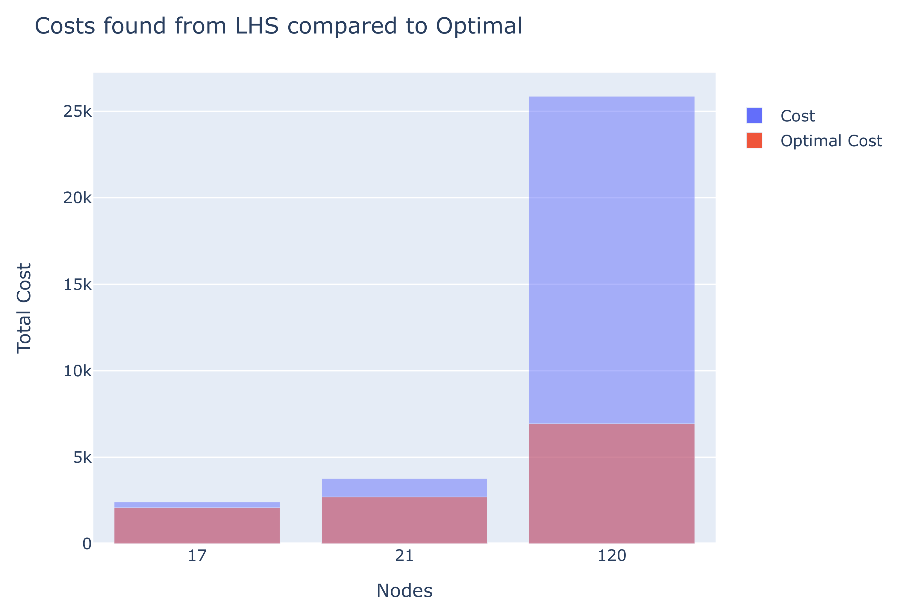
6.2. TSP Using LeapHybridSampler

Running the TSP problems using D-Wave’s LeapHybridSampler resulted in the metrics found in

Table 7. This table contains the average metrics gathered from experiments on TSP instances using D-Wave’s LeapHybridSampler.

Nodes	Solver	Runs	QAT (μs)	Run Time (μs)	Cost	Success Rate (%)
17	hybrid_binary_quadratic_model_version2	20	14,217.95	2,995,196.1	2417.15	100.0
21	hybrid_binary_quadratic_model_version2	20	7181.00	3,003,955.9	3775.75	100.0
120	hybrid_binary_quadratic_model_version2	5	107,764.40	75,028,024.6	25,871.20	100.0

. The “Nodes” column contains the number of nodes of the graphs, the “Solver” column shows the selected QPU that was used to solve the problem, and the “Runs” column gives the total number of times the experiment was executed. The “QAT” column shows the QPU access time, that is, the average time the quantum processing unit took to solve the problem over all runs. The “Run Time” column contains is the average total time (in microseconds) the solver took to solve the problem instance. The “Cost” column shows the average cost of the solution path from each run. Finally, the “Success Rate” column depicts the percentage of runs that provided a solution that did not violate any of the constraints. Table 7 shows that while the QPU access time is an increasing function of n, the results are again different from Table 4, since the hybrid computer did not access the QPU every time. We emphasize that the LeapHybridSampler successfully solved the gr120 problem from the TSPLIB, an instance with 120 nodes. The fact that the resulting paths were far from optimal can be attributed to the way LeapHybridSampler breaks the problems down to smaller instances, possibly losing important “shortcut” paths.

Figure 7 presents the average cost of the solution produced by the LeapHybridSampler, compared to the optimal solution for each problem. One can see that as the number of nodes of the graph increases, the solution produced by LeapHybridSampler deviates from the optimal even more. Additionally, the average cost of the solutions reached by the annealer exhibits significant discrepancies compared to the optimal solutions. This is in line with the findings from a very recent study [38] that also highlighted the difficulty faced by the D-Wave solvers when finding optimal solutions for TSP instances.

7. Discussion and Conclusions

In this work, we have considered various implementations, computational analyses, and comparisons of different versions of the D-Wave quantum annealer for the HCP and TSP problems. We extended our previous work by providing a complete matrix formulation for the HCP and TSP problems, and by introducing a normalization technique on the weight matrices. This technique helped avoid the constraint generated by the TSP graph’s weights overshadowing the other imposed constraints, causing D-Wave’s annealers to misbehave. We also ran some experiments on D-Wave’s annealers and came to the following conclusions:

• D-Wave’s Advantage_system4.1 is more efficient than the Advantage_system1.1 in its use of qubits for solving a problem and provides more consistently correct solutions;
• It is possible to run the Burma14 instance of the TSPLIB library on a quantum annealer using the aforementioned methods, although it cannot provide a “correct” solution because of the annealer’s limitations;
• The more connected a graph is, the fewer qubits are needed for it to be solved by the quantum annealers, as fewer constraints need to be imposed;
• Hybrid solvers always provide a correct solution to a problem and never break the constraints of a QUBO model, even for arbitrarily big problems.

The above conclusions are particularly significant, as they indicate that quantum annealers can solve TSP and HCP problems. With the current advancements in quantum computing, the prospect of using a quantum annealer for solving real-world TSP problems looks very promising, especially if quantum computers continue to scale at the rate we see today.

Our computational results indicate that our method is very promising. We intend to continue this line of research and extend its usage to a variety of problem classes, with emphasis on other variations of TSP problems, such as the traveling salesperson problem. Other possible improvements that we intend to evaluate experimentally include the introduction of suitable “phantom edges” on graphs that are not fully connected, in order to circumvent the addition of more constraints, as well as experimenting with more normalization methods for the TSP graph weights.

References

1. Feynman, R.P. Simulating physics with computers. Int. J. Theor. Phys. 1982, 21, 467–488. [Google Scholar] [CrossRef]
2. Shor, P.W. Polynomial-time algorithms for prime factorization and discrete logarithms on a quantum computer. SIAM Rev. 1999, 41, 303–332. [Google Scholar] [CrossRef]
3. Grover, L. A fast quantum mechanical algorithm for database search. In Proceedings of the Twenty-Eighth Annual ACM Symposium on the Theory of Computing, Philadelphia, PA, USA, 22–24 May 1996. [Google Scholar] [CrossRef] [Green Version]
4. Nielsen, M.A.; Chuang, I.L. Quantum Computation and Quantum Information; Cambridge University Press: Cambridge, UK, 2010. [Google Scholar]
5. Kadowaki, T.; Nishimori, H. Quantum annealing in the transverse Ising model. Phys. Rev. E 1998, 58, 5355. [Google Scholar] [CrossRef] [Green Version]
6. Kirkpatrick, S.; Gelatt, C.D.; Vecchi, M.P. Optimization by simulated annealing. Science 1983, 220, 671–680. [Google Scholar] [CrossRef] [PubMed]
7. Pakin, S. Performing fully parallel constraint logic programming on a quantum annealer. Theory Pract. Log. Program. 2018, 18, 928–949. [Google Scholar] [CrossRef] [Green Version]
8. Papalitsas, C.; Karakostas, P.; Andronikos, T.; Sioutas, S.; Giannakis, K. Combinatorial GVNS (General Variable Neighborhood Search) Optimization for Dynamic Garbage Collection. Algorithms 2018, 11, 38. [Google Scholar] [CrossRef] [Green Version]
9. Dong, Y.; Huang, Z. An improved noise quantum annealing method for TSP. Int. J. Theor. Phys. 2020, 59, 3737–3755. [Google Scholar] [CrossRef]
10. Choi, V. Minor-embedding in adiabatic quantum computation: I. The parameter setting problem. Quantum Inf. Process. 2008, 7, 193–209. [Google Scholar] [CrossRef] [Green Version]
11. Boothby, K.; Bunyk, P.; Raymond, J.; Roy, A. Next-generation topology of D-Wave quantum processors. arXiv 2020, arXiv:2003.00133. [Google Scholar]
12. D-Wave. D-Wave QPU Architecture: Topologies. Available online: https://docs.dwavesys.com/docs/latest/c_gs_4.html#pegasus-couplers (accessed on 3 January 2022).
13. Glover, F.; Kochenberger, G. A Tutorial on Formulating QUBO Models. arXiv 2018, arXiv:1811.11538. [Google Scholar]
14. Silva, C.; Aguiar, A.; Lima, P.; Dutra, I. Mapping a logical representation of TSP to quantum annealing. Quantum Inf. Process. 2021, 20, 386. [Google Scholar] [CrossRef]
15. Boros, E.; Hammer, P.L.; Tavares, G. Local search heuristics for quadratic unconstrained binary optimization (QUBO). J. Heuristics 2007, 13, 99–132. [Google Scholar] [CrossRef]
16. Newell, G.F.; Montroll, E.W. On the theory of the Ising model of ferromagnetism. Rev. Mod. Phys. 1953, 25, 353. [Google Scholar] [CrossRef]
17. Lucas, A. Ising formulations of many NP problems. Front. Phys. 2014, 2, 5. [Google Scholar] [CrossRef] [Green Version]
18. Neukart, F.; Compostella, G.; Seidel, C.; Von Dollen, D.; Yarkoni, S.; Parney, B. Traffic flow optimization using a quantum annealer. Front. ICT 2017, 4, 29. [Google Scholar] [CrossRef]
19. Filar, J.; Ejov, V. Flinders Hamiltonian Cycle Project. Available online: https://sites.flinders.edu.au/flinders-hamiltonian-cycle-project/graph-database/ (accessed on 3 January 2022).
20. Meringer, M. Fast generation of regular graphs and construction of cages. J. Graph Theory 1999, 30, 137–146. [Google Scholar] [CrossRef]
21. Shmoys, D.B.; Lenstra, J.; Kan, A.R.; Lawler, E.L. The Traveling Salesman Problem; John Wiley & Sons, Incorporated: Hoboken, NJ, USA, 1985; Volume 12. [Google Scholar]
22. Bianchi, L.; Dorigo, M.; Gambardella, L.M.; Gutjahr, W.J. A survey on metaheuristics for stochastic combinatorial optimization. Nat. Comput. 2009, 8, 239–287. [Google Scholar] [CrossRef] [Green Version]
23. Blum, C.; Roli, A. Metaheuristics in combinatorial optimization: Overview and conceptual comparison. ACM Comput. Surv. 2003, 35, 268–308. [Google Scholar] [CrossRef]
24. Papalitsas, C.; Giannakis, K.; Andronikos, T.; Theotokis, D.; Sifaleras, A. Initialization methods for the TSP with Time Windows using Variable Neighborhood Search. In Proceedings of the 6th International Conference on Information, Intelligence, Systems and Applications (IISA 2015), Corfu, Greece, 6–8 July 2015; pp. 1–6. [Google Scholar] [CrossRef]
25. Papalitsas, C.; Andronikos, T. Unconventional GVNS for Solving the Garbage Collection Problem with Time Windows. Technologies 2019, 7, 61. [Google Scholar] [CrossRef] [Green Version]
26. Papalitsas, C.; Andronikos, T.; Karakostas, P. Studying the Impact of Perturbation Methods on the Efficiency of GVNS for the ATSP. In Variable Neighborhood Search; Springer International Publishing: New York, NY, USA, 2019; pp. 287–302. [Google Scholar] [CrossRef]
27. Papalitsas, C.; Karakostas, P.; Andronikos, T. A Performance Study of the Impact of Different Perturbation Methods on the Efficiency of GVNS for Solving TSP. Appl. Syst. Innov. 2019, 2, 31. [Google Scholar] [CrossRef] [Green Version]
28. Gan, R.; Guo, Q.; Chang, H.; Yi, Y. Improved ant colony optimization algorithm for the traveling salesman problems. J. Syst. Eng. Electron. 2010, 21, 329–333. [Google Scholar] [CrossRef]
29. Aono, M.; Zhu, L.; Hara, M. Amoeba-based neurocomputing for 8-city traveling salesman problem. Int. J. Unconv. Comput. 2011, 7, 463–480. [Google Scholar]
30. Martoňák, R.; Santoro, G.E.; Tosatti, E. Quantum annealing of the traveling-salesman problem. Phys. Rev. E 2004, 70, 057701. [Google Scholar] [CrossRef] [PubMed] [Green Version]
31. Papalitsas, C.; Andronikos, T.; Giannakis, K.; Theocharopoulou, G.; Fanarioti, S. A QUBO Model for the Traveling Salesman Problem with Time Windows. Algorithms 2019, 12, 224. [Google Scholar] [CrossRef] [Green Version]
32. Warren, R.H. Solving the traveling salesman problem on a quantum annealer. SN Appl. Sci. 2020, 2, 1–5. [Google Scholar] [CrossRef] [Green Version]
33. Qubovert. The One-Stop Package for Formulating, Simulating, and Solving Problems in Boolean and Spin Form. Available online: https://qubovert.readthedocs.io/en/latest/index.html (accessed on 3 January 2022).
34. Han, J.; Kamber, M.; Pei, J. Data Preprocessing. In Data Mining, 3rd ed.; Han, J., Kamber, M., Pei, J., Eds.; The Morgan Kaufmann Series in Data Management Systems; Morgan Kaufmann: Burlington, MA, USA, 2012; pp. 83–124. [Google Scholar] [CrossRef]
35. McGeoch, C.; Farré, P. The D-Wave Advantage System: An Overview; Technical Report; D-Wave Systems Inc.: Burnaby, BC, Canada, 2020. [Google Scholar]
36. D-Wave Systems. Advantage_system1.1 Solver Decommissioned. 2021. Available online: https://docs.dwavesys.com/docs/latest/rn_feature_descriptions.html#advantage-system1-1-solver-decommissioned (accessed on 30 November 2021).
37. McGeoch, C.; Farré, P. The Advantage System: Performance Update; Technical Report; D-Wave Systems Inc.: Burnaby, BC, Canada, 2021. [Google Scholar]
38. Warren, R.H. Solving combinatorial problems by two DWave hybrid solvers: A case study of traveling salesman problems in the TSP Library. arXiv 2021, arXiv:2106.05948. [Google Scholar]
39. Reinelt, G. TSPLIB—A Traveling Salesman Problem Library. ORSA J. Comput. 1991, 3, 376–384. [Google Scholar] [CrossRef]
40. LeapHybridSampler. Available online: https://docs.ocean.dwavesys.com/projects/system/en/latest/reference/samplers.html#leaphybridsampler (accessed on 30 November 2021).
41. Leap’s Hybrid Solvers Documentation. Available online: https://docs.ocean.dwavesys.com/en/latest/overview/hybrid.html#leap-s-hybrid-solvers (accessed on 30 November 2021).
42. Leap’s Hybrid Solvers Documentation. Available online: https://docs.dwavesys.com/docs/latest/doc_leap_hybrid.html#id1 (accessed on 30 November 2021).
Figure 1. The 4-node graph G 1 of Example 1.
Mathematics 10 01294 g001
Figure 2. LeapHybridSampler returned a valid solution in all 10 normalized instances, but failed to do so in all 10 instances that were not normalized.
Mathematics 10 01294 g002
Figure 3. The number of qubits used in the embedding as a function of the number of nodes.
Mathematics 10 01294 g003
Figure 4. The average QPU access time as a function of the number of nodes.
Mathematics 10 01294 g004
Figure 5. The average number of qubits used for Burma14 on the QPU.
Mathematics 10 01294 g005
Figure 6. The number of qubits as a function of the number of edges in a graph with 14 nodes.
Mathematics 10 01294 g006
Figure 7. Comparison of the solutions produced by LeapHybridSampler and the optimal ones.
Mathematics 10 01294 g007