Article

Approximation by Tensor-Product Kind Bivariate Operator of a New Generalization of Bernstein-Type Rational Functions and Its GBS Operator

by
Esma Yıldız Özkan
1,* and
Gözde Aksoy
2
1
Department of Mathematics, Faculty of Science, Gazi University, 06500 Ankara, Turkey
2
Department of Mathematics, Graduate School of Natural and Applied Sciences, Gazi University, 06500 Ankara, Turkey
*
Author to whom correspondence should be addressed.
Mathematics 2022, 10(9), 1418; https://doi.org/10.3390/math10091418
Submission received: 1 April 2022 / Revised: 16 April 2022 / Accepted: 20 April 2022 / Published: 22 April 2022
(This article belongs to the Special Issue Mathematical Inequalities, Models and Applications)

Abstract

:
We introduce a tensor-product kind bivariate operator of a new generalization of Bernstein-type rational functions and its GBS (generalized Boolean sum) operator, and we investigate their approximation properties by obtaining their rates of convergence. Moreover, we present some graphical comparisons visualizing the convergence of tensor-product kind bivariate operator and its GBS operator.

1. Introduction

Bernstein-type rational functions were defined by Balázs in [1] as follows:
R n f ; u = 1 1 + a n u n k = 0 n f k b n n k ( a n u ) k , u 0 , n N ,
where a n and b n are suitably chosen non-negative real sequences such that b n = n a n for each n N , and f is a real-valued function on 0 , .
In [2], Atakut and İspir introduced the bivariate operator of the Bernstein-type rational functions defined by (1) as follows:
R n , m ( f ; u , v ) = j = 0 n k = 0 m f j b n , k b m n j m k ( a n u ) j ( a m v ) k 1 + a n u n 1 + a m v m , u , v 0 , n , m N ,
where a n , a m , b n and b m are suitably chosen non-negative sequences such that b h = h a h for h = n , m N , and f is a real-valued function on 0 , × 0 , . They obtained an estimate by means of the usual first modulus of continuity and proved an asymptotic approximation theorem with the classical methods. Moreover, Atakut [3] presented some convergence results associated with the derivatives of the operator R n , m defined by (2).
Recently, a new generalization of Bernstein-type rational functions has been defined in [4] by:
R n G ( f ; u ) = k = 0 n f k γ n n k ( α n u ) k ( β n ) n k β n + α n u n , u 0 , n N ,
where f is a real-valued continuous function on 0 , , and α n , β n and γ n are non-negative real sequences such that γ n = n α n satisfying the following properties:
lim n α n = 0 , lim n β n = 1 and lim n γ n = .
The operator R n G is a linear and positive operator. When β n = 1 , α n = a n and γ n = b n , it is reduced to the Bernstein-type rational functions given by (1). Therefore, it is a generalization of the Bernstein-type rational functions. Its Korovkin-type approximation results have been investigated in [4].
Recently, the approximation properties of lots of bivariate operators have been investigated. Readers can see the following references for details [5,6,7,8,9,10,11,12,13,14,15].
In this study, we introduce a tensor-product kind bivariate operator and its associated GBS (generalized Boolean sum) operator of the generalized Bernstein-type rational function R n G defined by (3), which is a generalization of the bivariate operator R n , m defined by (2). Moreover, we investigate their approximation properties on rectangular region 0 , r 1 × 0 , r 2 such that r 1 , r 2 > 0 . Lastly, we present an application including illustrative graphics visualizing the convergence of the tensor-product kind bivariate operator and its GBS operator, which also compare their convergence with the bivariate operator R n , m defined by (2).

2. Construction of Tensor-Product Kind Bivariate Operator

In this part, we introduce a tensor-product kind bivariate operator of the generalized Bernstein-type rational function R n G defined by (3) and investigate its approximation properties.
Let α 1 n , α 2 m , β 1 n , β 2 m , γ 1 n and γ 2 m be non-negative real sequences such that γ ϕ h = h α ϕ h for ( ϕ , h ) = ( 1 , n ) , ( 2 , m ) , fulfilling the following conditions:
lim n , m α ϕ h = 0 , lim n , m β ϕ h = 1 and lim n , m γ ϕ h = .
Let f be a real-valued continuous function on 0 , × 0 , . We define the following tensor-product kind bivariate operator:
R n , m G ( f ; u , v ) = j = 0 n k = 0 m f j γ 1 n , k γ 2 m s n , j u s m , k v , u , v 0 , n , m N ,
where s n , j u = n j ( α 1 n u ) j ( β 1 n ) n j β 1 n + α 1 n u n , s m , k v = m k ( α 2 m v ) k ( β 2 m ) m k β 2 m + α 2 m v m . For any ϕ , φ R and any real-valued continuous functions f , h on 0 , × 0 , , we have the following relation:
R n , m G ( ϕ f + φ h ; u , v ) = ϕ R n , m G ( f ; u , v ) + φ R n , m G ( h ; u , v ) ,
and if f is non-negative, then R n , m G ( f ; . ) is non-negative. Therefore, the bivariate operator R n , m G is linear and positive. By denoting:
x R n G f τ , ς ; u , ς : = j = 0 n f j γ 1 n , ς s n , j u ,
y R m G f τ , ς ; τ , v : = k = 0 m f τ , k γ 2 m s m , k v ,
the bivariate operator R n , m G is the tensorial product of x R n G and y R m G such that:
R n , m G = x R n G y R m G = y R m G x R n G .
Indeed, by denoting g τ , v : = y R m G f τ , ς ; τ , v , we obtain:
x R n G y R m G f τ , ς ; τ , v ; u , v = x R n G g τ , v ; u , v = j = 0 n g j γ 1 n , v s n , j u = j = 0 n k = 0 m f j γ 1 n , k γ 2 m s m , k v s n , j u = j = 0 n k = 0 m f j γ 1 n , k γ 2 m s n , j u s m , k v = R n , m G ( f τ , ς ; u , v ) .
Similarly, we have the following relation:
y R m G x R n G f τ , ς ; u , ς ; u , v = R n , m G ( f τ , ς ; u , v ) .
If α ϕ h = a h , γ ϕ h = b h and β ϕ h = 1 for ( ϕ , h ) = ( 1 , n ) , ( 2 , m ) , then the tensor-product kind operator R n , m G is reduced to the bivariate operator R n , m defined by (2). Therefore, the tensor-product kind operator R n , m G is a generalization of the bivariate operator R n , m defined by (2)
Now, we give some auxilary results:
Lemma 1.
Let R n , m G be the operator defined by (6) and ψ i , j ( τ , ς ) = τ i ς j , i , j = 0 , 1 , 2 , be the bivariate test functions. Then, we have the following equalities:
R n , m G ( ψ 0 , 0 ; u , v ) = 1 ,
R n , m G ( ψ 1 , 0 ; u , v ) = u β 1 n + α 1 n u ,
R n , m G ( ψ 0 , 1 ; u , v ) = v β 2 m + α 2 m v ,
R n , m G ( ψ 2 , 0 ; u , v ) = 1 1 n u 2 β 1 n + α 1 n u 2 + u γ 1 n β 1 n + α 1 n u ,
R n , m G ( ψ 0 , 2 ; u , v ) = 1 1 m v 2 β 2 m + α 2 m v 2 + v γ 2 m β 2 m + α 2 m v .
Proof. 
By the proof of Lemma 1 of [4], we can write:
R n , m G ( ψ 0 , 0 ; u , v ) = j = 0 n k = 0 m 1 . s n , j u s m , k v = 1
R n , m G ( ψ 1 , 0 ; u , v ) = j = 1 n j γ 1 n s n , j u k = 0 m s m , k v = u β 1 n + α 1 n u j = 0 n 1 s n 1 , j u k = 0 m s m , k v = u β 1 n + α 1 n u ,
R n , m G ( ψ 2 , 0 ; u , v ) = j = 0 n k = 0 m j γ 1 n 2 s n , j u s m , k v = j = 0 n j γ 1 n 2 s n , j u k = 0 m s m , k v = 1 1 n u 2 β 1 n + α 1 n u 2 j = 0 n 2 s n 2 , j u k = 0 m s m , k v + u γ 1 n β 1 n + α 1 n u j = 0 n 1 s n 1 , j u k = 0 m s m , k v = 1 1 n u 2 β 1 n + α 1 n u 2 + u γ 1 n β 1 n + α 1 n u .
Similarly, R n , m G ( ψ 0 , 1 ; u , v ) and R n , m G ( ψ 0 , 2 ; u , v ) can be easily calculated by interchanging the roles of the components j , n and u of s n , j u with k, m and v and the components k, m and v of s m , k v with j , n and u, respectively. □
Remark 1.
From Lemma 1, we obtain:
R n , m G ( τ u ; u , v ) = 1 β 1 n u β 1 n + α 1 n u α 1 n u 2 β 1 n + α 1 n u ,
R n , m G ( ς v ; u , v ) = 1 β 2 m v β 2 m + α 2 m v α 2 m v 2 β 2 m + α 2 m v ,
R n , m G ( τ u 2 ; u , v ) = β 1 n u γ 1 n β 1 n + α 1 n u 2 + α 1 n + β 1 n 1 2 1 n u 2 β 1 n + α 1 n u 2 + 2 α 1 n β 1 n 1 u 3 β 1 n + α 1 n u 2 + α 1 n u 4 β 1 n + α 1 n u 2 ,
R n , m G ( ς y 2 ; u , v ) = β 2 m v γ 2 m β 2 m + α 2 m v 2 + α 2 m + β 2 m 1 2 1 m v 2 β 2 m + α 2 m v 2 + 2 α 2 m β 2 m 1 v 3 β 2 m + α 2 m v 2 + α 2 m v 4 β 2 m + α 2 m v 2 .

3. Approximation Results

In this part, we firstly present a Volkov-type result for the tensor-product kind bivariate operator R n , m G .
Let A 0 , × 0 , be a compact set of R 2 , and C A be the space of all real-valued continuous functions f on A with the supremum norm f = sup f u , v : u , v A .
Theorem 1.
Let R n , m G , n , m N , be the tensor-product kind bivariate operator defined by (6) and α 1 n , α 2 m , β 1 n , β 2 m , γ 1 n and γ 2 m be real sequences fulfilling the condition (5). Then, for all f C 0 , r 1 × 0 , r 2 , r 1 , r 2 > 0 , R n , m G ( f ) converges uniformly to f on 0 , r 1 × 0 , r 2 .
Proof. 
By Lemma 1, the theorem can be proved by considering Volkov’s theorem in [16] with similar methods to the proof of Theorem 1 of [4]; therefore, we omit its proof. □
Now, we obtain inequalities estimating the error of the approximation by the tensor-product kind bivariate operator R n , m G defined by (6).
The complete modulus of continuity for bivariate functions f C A is defined as follows:
ω f ; μ 1 , μ 2 = sup f τ , ς f u , v : τ u μ 1 , ς v μ 2 , τ , ς , u , v A ,
where μ 1 , μ 2 > 0 .
Moreover, the partial modulus of continuity according to x and y are defined by:
ω 1 f ; μ 1 = sup f τ , v f u , v : τ u μ 1 , τ , v , u , v A , ω 2 f ; μ 2 = sup f u , ς f u , v : ς v μ 2 , u , ς , u , v A ,
which fulfill the properties of the classical modulus of continuity. The details of the modulus of continuity for the bivariate functions can be found in [17].
Secondly, we estimate the rate of convergence of the tensor-product kind bivariate operator R n , m G defined in (6) by using the complete modulus of continuity.
Theorem 2.
Let f C 0 , r 1 × 0 , r 2 , r 1 , r 2 > 0 . Then, the following inequality holds:
R n , m G ( f ; u , v ) f u , v 4 ω f ; μ n u , μ m v ,
where μ n u : = R n , m G ( τ u 2 ; u , v ) 1 / 2 and μ m v : = R n , m G ( ς v 2 ; u , v ) 1 / 2 .
Proof. 
Using the linearity and the positivity of the operator R n , m G and taking properties of the complete modulus of continuity into account, we can write:
R n , m G ( f ; u , v ) f u , v R n , m G f τ , ς f u , v ; u , v ω f ; μ 1 , μ 2 1 + 1 μ 1 R n , m G τ u ; u , v + 1 μ 2 R n , m G ς v ; u , v + 1 μ 1 μ 2 R n , m G τ x ς v ; u , v .
Applying the Cauchy–Schwarz inequality to (7), we obtain:
R n , m G ( f ; u , v ) f u , v ω f ; μ 1 , μ 2 1 + 1 μ 1 R n , m G τ u 2 ; u , v 1 / 2 + 1 μ 2 R n , m G ς v 2 ; u , v 1 / 2 + 1 μ 1 μ 2 R n , m G τ u 2 ς v 2 ; u , v 1 / 2 .
In (8), by considering Lemma 1 and choosing μ 1 = : μ n u : = R n , m G ( τ u 2 ; u , v ) 1 / 2 and μ 2 = : μ m v : = R n , m G ( ς v 2 ; u , v ) 1 / 2 , we complete the proof of the theorem. □
We present in the following theorem the estimation of the rate of the convergence by the tensor-product kind bivariate operator R n , m G defined in (6) by means of the partial modulus of continuities.
Theorem 3.
Let f C 0 , r 1 × 0 , r 2 , r 1 , r 2 > 0 . Then, the following inequality is valid:
R n , m G ( f ; u , v ) f u , v 2 ω 1 f ; μ n u + ω 2 f ; μ m v .
Proof. 
Considering the definition of the partial modulus of continuity and using the Cauchy–Schwarz inequality, we can write:
R n , m G ( f ; u , v ) f u , v R n , m G f τ , ς f u , v ; u , v R n , m G f τ , ς f u , ς ; u , v + R n , m G f u , ς f u , v ; u , v ω 1 f ; μ 1 1 + 1 μ 1 R n , m G τ u ; u , v + ω 2 f ; μ 2 1 + 1 μ 2 R n , m G ς v ; u , v ω 1 f ; μ 1 1 + 1 μ 1 R n , m G ( τ u 2 ; u , v ) 1 / 2 + ω 2 f ; μ 2 1 + 1 μ 2 R n , m G ( ς v 2 ; u , v ) 1 / 2 .
Choosing μ 1 = : μ n u : = R n , m G ( τ u 2 ; u , v ) 1 / 2 and μ 2 = : μ m v : = R n , m G ( ς v 2 ; u , v ) 1 / 2 , we complete the proof. □
Now, we investigate the rate of convergence of the operator R n , m G defined in (6) with the help of functions of the Lipschitz type.
Any function f C A is called a function of Lipschitz type and denoted by f L i p M ( a , b ) if there exists an M > 0 such that:
f τ , ς f u , v M τ u a ς v b ,
where ( τ , ς ) , ( u , v ) A are arbitrary and 0 < a , b 1 .
Theorem 4.
Let f L i p M ( a , b ) . Then, there exists an M > 0 such that:
R n , m G ( f ; u , v ) f u , v M μ n u a μ m v b ,
for all ( x , y ) 0 , r 1 × 0 , r 2 , where μ n u : = R n , m G ( τ u 2 ; u , v ) 1 / 2 and μ m v : = R n , m G ( ς v 2 ; u , v ) 1 / 2 .
Proof. 
By the hypothesis of the theorem, we can write:
R n , m G ( f ; u , v ) f u , v R n , m G f τ , ς f u , v ; u , v M R n , m G ( τ u a ς v b ; u , v ) = M R n , m G ( τ u a ; x , y ) × R n , m G ( ς v b ; u , v ) .
Respectively, applying the Hölder’s inequality to the last inequality for p 1 = 2 a , q 1 = 2 2 a , p 2 = 2 b and q 2 = 2 2 b such that 1 p i + 1 q i = 1 , i = 1 , 2 , we obtain:
R n , m G ( f ; u , v ) f u , v M R n , m G ( τ u 2 ; u , v ) a / 2 R n , m G ( 1 ; u , v ) ( 2 a ) / 2 × R n , m G ( ς v 2 ; u , v ) b / 2 R n , m G ( 1 ; u , v ) ( 2 b ) / 2 = M μ n u a μ m v b ,
which completes the proof of the theorem. □

4. GBS Operator

In this part, we construct the GBS operator associated with the tensor-product kind bivariate operator R n , m G .
We recall some basic notations given by Bögel. The details of which can be found in references [18,19,20].
Let A be a compact subset of R 2 . A real-valued function on A is called Bögel-continuous function at τ , ς A if:
Δ u , v f τ , ς ; u , v = 0 ,
where Δ u , v f τ , ς ; u , v denotes the mixed difference defined by:
Δ u , v f τ , ς ; u , v = f u , v f u , ς f τ , v + f τ , ς .
Let A be a subset of R 2 . A real-valued function on A is Bögel-bounded function if there exists an M > 0 such that:
Δ u , v f τ , ς ; u , v M ,
for all τ , ς , u , v A .
Let A be a compact subset of R 2 . Then, each Bögel-continuous function is a Bögel-bounded function. Let C B A denote the space of all the real-valued Bögel-continuous functions defined on A endowed with the following norm:
f B = s u p Δ u , v f τ , ς ; u , v : u , v , τ , ς A .
It is obvious that C A C B A .
For f C 0 , r 1 × 0 , r 2 , r 1 , r 2 > 0 , we introduce the GBS (generalized Boolean sum) operator associated with the operator R n , m G by:
B n , m G ( f τ , ς ; u , v ) = R n , m G f ( u , ς ) + f ( τ , v ) f ( τ , ς ) ; u , v ,
for all ( τ , ς ) , ( u , v ) 0 , r 1 × 0 , r 2 and n , m N . We can definitely write:
B n , m G ( f τ , ς ; u , v ) = j = 0 n k = 0 m s n , j u s m , k v × f u , k γ 2 m + f j γ 1 n , v f j γ 1 n , k γ 2 m
where s n , j u = n j ( α 1 n u ) j ( β 1 n ) n j β 1 n + α 1 n u n , s m , k v = m k ( α 2 m v ) k ( β 2 m ) m k β 2 m + α 2 m v m and α 1 n , α 2 m , β 1 n , β 2 m , γ 1 n and γ 2 m are non-negative real sequences such that γ ϕ h = h α ϕ h for ( ϕ , h ) = ( 1 , n ) , ( 2 , m ) fulfilling the condition of (5).
It is clear that B n , m G maps C B 0 , r 1 × 0 , r 2 into itself, and it is linear and positive.
The mixed modulus of smoothness of f C B A is defined in [21] by:
ω m i x e d ( f ; u , v ) = sup { Δ ( u , v ) f τ , ς ; u , v : τ u < μ 1 , ς v < μ 2 , ( τ , ς ) , ( u , v ) A } .
Theorem 5.
For any f C B 0 , r 1 × 0 , r 2 , the following inequality is valid:
B n , m G ( f ; u , v ) f ( u , v ) 4 ω m i x e d ( f ; μ n u , μ m v )
where μ n u : = R n , m G ( τ u 2 ; u , v ) 1 / 2 and μ m v : = R n , m G ( ς v 2 ; u , v ) 1 / 2 .
Proof. 
By (11) and for λ 1 , λ 2 > 0 , the mixed modulus of smoothness ω m i x e d possesses the following property:
ω m i x e d ( f ; λ 1 μ 1 , λ 2 μ 2 ) 1 + λ 1 1 + λ 2 ω m i x e d f ; μ 1 , μ 2 ,
by which for all ( τ , ς ) , ( u , v ) 0 , r 1 × 0 , r 2 , we obtain:
Δ ( u , v ) f τ , ς ; u , v f ( u , v ) f ( u , ς ) f ( τ , v ) + f ( τ , ς ) ω m i x e d ( f ; τ u , ς v ) 1 + τ u μ 1 1 + ς v μ 2 ω m i x e d f ; μ 1 , μ 2 .
By (9), we can write:
f ( u , ς ) + f ( τ , v ) f ( τ , ς ) = f ( u , v ) Δ ( u , v ) f τ , ς ; u , v .
Considering the definition of R n , m G and B n , m G , we obtain:
B n , m G f τ , ς ; u , v = R n , m G f ( u , ς ) + f ( τ , v ) f ( τ , ς ) ; u , v = f ( u , v ) R n , m G ψ 0 , 0 ; u , v R n , m G Δ ( u , v ) f τ , ς ; u , v ; u , v .
By (12) and taking the Cauchy–Schwarz inequality into account, we obtain:
B n , m G ( f ; u , v ) f ( u , v ) [ R n , m G 1 ; u , v + 1 μ 1 ( R n , m G ( ( τ u ) 2 ; u , v ) ) 1 / 2 + 1 μ 2 ( R n , m G ( ( ς v ) 2 ; u , v ) ) 1 / 2 + 1 μ 1 μ 2 ( R n , m G ( ( τ u ) 2 ; u , v ) R n , m G ( ( ς v ) 2 ; u , v ) ) 1 / 2 ] × ω m i x e d f ; μ 1 , μ 2 .
Choosing μ n u : = R n , m G ( τ u 2 ; u , v ) 1 / 2 and μ m v : = R n , m G ( ς v 2 ; u , v ) 1 / 2 , we obtain the desired result. □
Now, we recall the Bögel-continuous functions of Lipschitz type. For f C B A , ( τ , ς ) , ( u , v ) A and 0 < a , b 1 , if there exists an M > 0 such that:
Δ ( u , v ) f τ , ς ; u , v M τ u a ς v b ,
then f is called a Bögel-continuous function of Lipschitz type and denoted by L i p M B a , b .
Theorem 6.
Let f L i p M B a , b . Then, for all ( u , v ) 0 , r 1 × 0 , r 2 , we have the following inequality:
B n , m G ( f ; u , v ) f ( u , v ) M μ n u a μ m v b , M > 0 ,
where μ n u : = R n , m G ( τ u 2 ; u , v ) 1 / 2 and μ m v : = R n , m G ( ς v 2 ; u , v ) 1 / 2 .
Proof. 
Since:
B n , m G ( f ; u , v ) = R n , m G f ( u , ς ) + f ( τ , v ) f ( τ , ς ) ; u , v = R n , m G f ( u , v ) Δ ( u , v ) f τ , ς ; u , v ; u , v = f ( u , v ) R n , m G ψ 0 , 0 ; u , v R n , m G Δ ( u , v ) f τ , ς ; u , v ; u , v ,
we can write:
B n , m G ( f ; u , v ) f ( u , v ) R n , m G Δ ( u , v ) f τ , ς ; u , v ; u , v M R n , m G ( τ u a ς v b ; u , v ) = M R n , m G ( τ u a ; u , v ) × R n , m G ( ς v b ; u , v ) .
Applying the Hölder’s inequality to the last inequality by choosing p 1 = 2 a , q 1 = 2 2 a , p 2 = 2 b and q 2 = 2 2 b such that 1 p i + 1 q i = 1 , i = 1 , 2 , we obtain:
B n , m G ( f ; u , v ) f u , v M R n , m G ( τ u 2 ; u , v ) a / 2 R n , m G ( 1 ; u , v ) ( 2 a ) / 2 × R n , m G ( ς v 2 ; u , v ) b / 2 R n , m G ( 1 ; u , v ) ( 2 b ) / 2 = M μ n u a μ m v b ,
which is the desired result. □

5. Graphical Comparisons

Let φ u , v = u v 2 such that u , v 0 , 3 × 0 , 3 .
1. Let us choose n = m , α ϕ h = n 1 / 2 , γ ϕ h = n 1 / 2 and β ϕ h = 1 5 n 1 such that ( ϕ , h ) = ( 1 , n ) , ( 2 , m ) , n , m = 1 , 2 , . . .
Figure 1 compares the approximation of R 5 , 5 G φ ; u , v (red), R 25 , 25 G φ ; u , v (yellow) and R 75 , 75 G φ ; u , v (green) to φ u , v (blue) on 0 , 3 × 0 , 3 . For increasing value of n, the approximation of R n , n G φ ; u , v to φ u , v becomes better.
Figure 2 compares the approximation of B 5 , 5 G φ ; u , v (red), B 25 , 25 G φ ; u , v (yellow) and B 75 , 75 G φ ; u , v (green) to φ u , v (blue) on 0 , 3 × 0 , 3 . Similarly, for increasing value of n, the approximation of B n , n G φ ; u , v to φ u , v becomes better.
2. Let us choose n = m = 75 , α ϕ h = n 1 / 2 , γ ϕ h = n 1 / 2 and β 1 = β ϕ h = 1 5 n 1 , β 2 = β ϕ h = 1 10 n 1 and β 2 = β ϕ h = 1 15 n 1 such that ( ϕ , h ) = ( 1 , n ) , ( 2 , m ) , n , m = 1 , 2 ,
Figure 3 compares the approximation of R 75 , 75 G φ ; u , v ; β 1 (red), R 75 , 75 G φ ; u , v ; β 2 (yellow) and R 75 , 75 G φ ; u , v ; β 3 (green) to φ u , v (blue) on 0 , 3 × 0 , 3 . One can see that the approximation of R 75 , 75 G φ ; u , v ; β 3 (green) to φ u , v (blue) is better than others.
Figure 4 compares the approximation of B 75 , 75 G φ ; u , v ; β 1 (red), B 75 , 75 G φ ; u , v ; β 2 (yellow) and B 75 , 75 G φ ; u , v ; β 3 (green) to φ u , v (blue) on 0 , 3 × 0 , 3 . One can see that the approximations of B 75 , 75 G φ ; u , v ; β 1 (red) and B 75 , 75 G φ ; u , v ; β 3 (green) are better in places of the sub-region of the region than B 75 , 75 G φ ; u , v ; β 2 (yellow).
3. Let us choose n = m , α ϕ h = n 1 / 2 , γ ϕ h = n 1 / 2 and β ϕ h = 1 5 n 1 such that ( ϕ , h ) = ( 1 , n ) , ( 2 , m ) , n , m = 1 , 2 , . . .
Figure 5, compares the approximation of the operators R 75 , 75 φ ; u , v (green), R 75 , 75 G φ ; u , v (red) and B 75 , 75 G φ ; u , v (yellow) to φ u , v (blue) on 0 , 3 × 0 , 3 . One can see that the approximation of B 75 , 75 G φ ; u , v ; β 2 (yellow) to φ u , v (blue) is the best. B 75 , 75 G φ ; u , v ; β 2 (yellow) is so close to φ u , v (blue) that it almost coincides.

6. Conclusions

In this paper, we have introduced the tensor-product kind bivariate operator R n , m G of the generalized Bernstein-type rational function R n G defined in [4] and its GBS (generalized Boolean sum) operator B n , m G , and we have investigated their approximation properties on rectangular region 0 , r 1 × 0 , r 2 such that r 1 , r 2 > 0 . Moreover, we have given some graphical comparisons visualizing the convergence of the tensor-product kind bivariate operator and its GBS operator, which also compare their convergence with the bivariate operator R n , m defined in [2].
The results of this paper demonstrate that the GBS operator B n , m G possesses at least a better approximation than the tensor-product kind bivariate operator R n , m G , while the tensor-product kind bivariate operator R n , m G has at least a better approximation than the bivariate operator R n , m defined in [2].

Author Contributions

Conceptualization, E.Y.Ö.; methodology, E.Y.Ö. and G.A.; software, E.Y.Ö.; validation, E.Y.Ö. and G.A.; investigation, E.Y.Ö. and G.A.; resources, E.Y.Ö. and G.A.; data curation, E.Y.Ö.; writing—original draft preparation, E.Y.Ö. and G.A.; writing—review and editing, E.Y.Ö.; visualization, E.Y.Ö.; supervision, E.Y.Ö. All authors have read and agreed to the published version of the manuscript.

Funding

This research received no external funding.

Institutional Review Board Statement

Not applicable.

Informed Consent Statement

Not applicable.

Data Availability Statement

All data of this article are included in the text.

Acknowledgments

The authors are grateful to all the referees contributed to the best presentation of the paper with their valuable comments.

Conflicts of Interest

The authors declare no conflict of interest.

References

  1. Balázs, K. Approximation by Bernstein type rational funcitons. Acta Math. Acad. Sci. Hung. 1975, 26, 123–124. [Google Scholar] [CrossRef]
  2. Atakut, Ç.; İspir, N. On Bernstein type rational functions of two variables. Math. Slovaca 2004, 54, 291–301. [Google Scholar] [CrossRef]
  3. Atakut, Ç. On derivatives Bernstein type rational functions of two variables. Appl. Math. Comput. 2011, 218, 673–677. [Google Scholar] [CrossRef]
  4. Özkan, E.Y.; Aksoy, G. On a new generalization of Bernstein-type rational functions and its approximation. Mathematics 2022, 10, 973. [Google Scholar] [CrossRef]
  5. Acu, A.M.; Acar, T.; Muraru, C.-V.; Radu, V.A. Some approximation properties by a class of bivariate operators. Math. Methods Appl. Sci. 2018, 42, 5551–5565. [Google Scholar] [CrossRef]
  6. Agrawal, P.N.; Acu, A.M.; Chauhan, R.; Garg, T. Approximation of Bögel continuous functions and deferred weighted A-statistical convergence by Bernstein-Kantorovich type operators on a triangle. J. Math. Inequal. 2021, 15, 1695–1711. [Google Scholar] [CrossRef]
  7. Başcanbaz-Tunca, G.; Erençin, A.; Olgun, A. Quantitative estimates for bivariate Stancu operators. Math. Methods Appl. Sci. 2019, 42, 5241–5250. [Google Scholar] [CrossRef]
  8. Agrawal, P.N.; Kajla, A.; Kumar, D. Modified ρ-Bernstein operators for functions of two variables. Numer. Funct. Anal. Optim. 2021, 42, 1073–1095. [Google Scholar] [CrossRef]
  9. İspir, N. Quantitative estimates for GBS operators of Chlodowsky-Szász type. Filomat 2017, 31, 1175–1184. [Google Scholar] [CrossRef]
  10. Özkan, E.Y. Approximation properties of bivariate complex q-Balazs-Szabados operators of tensor product kind. J. Inequal. Appl. 2014, 2014, 20. [Google Scholar] [CrossRef] [Green Version]
  11. Özkan, E.Y. Approximation by complex bivariate Balazs-Szabados operators. Bull. Malays. Math. Sci. Soc. 2016, 39, 1–16. [Google Scholar] [CrossRef]
  12. Özkan, E.Y. Qantitative estimates for the tensor product (p,q)-Balázs-Szabados operators and associated generalized Boolean sum operators. Filomat 2020, 34, 779–793. [Google Scholar] [CrossRef]
  13. Cai, Q.-B.; Zhou, Z. Durrmeyer type (p,q)-Baskakov operators for functions of one and two variables. J. Comput. Anal. Appl. 2019, 27, 481–501. [Google Scholar]
  14. Srivastava, H.M.; Ansari, K.J.; Özger, F.; Ödemiş Özger, Z. A Link between approximation theory and summability methods via four-dimensional infinite matrices. Mathematics 2021, 9, 1895. [Google Scholar] [CrossRef]
  15. Cai, Q.-B.; Ansari, K.J.; Temizer Ersoy, M.; Özger, F. Statistical blending-type approximation by a class of operators that includes shape parameters λ and α. Mathematics 2022, 10, 1149. [Google Scholar] [CrossRef]
  16. Volkov, V.I. On the convergence of sequences of linear positive operators in the space of continuous functions of two variables. Dokl. Akad. Nauk. SSSR (N.S.) 1957, 115, 17–19. (In Russian) [Google Scholar]
  17. Anastassiou, G.A.; Gal, S.G. Approximation Theory: Moduli of Continuity and Global Smoothness Preservation; Birkhäuser: Boston, MA, USA, 2000. [Google Scholar]
  18. Bögel, K. Mehr dimensionale Differentiation von Funktionen mehrerer Veränderlicher. J. Reine Angew. Math. 1934, 170, 197–217. [Google Scholar] [CrossRef]
  19. Bögel, K. Über die mehrdimensionale Integration und beschränkte Variation. J. Reine Angew. Math. 1935, 173, 5–29. [Google Scholar] [CrossRef]
  20. Bögel, K. Über die mehrdimensionale Differentiation. Jahresber. Dtsch. Math. Ver. 1962, 65, 45–71. [Google Scholar]
  21. Badea, C.; Cottin, C. Korovkin-type theorems for generalized Boolean sum operators. Approximation theory (Kecskemét, 1900). Colloq. Math. Soc. János Bolyai. 1990, 58, 51–68. [Google Scholar]
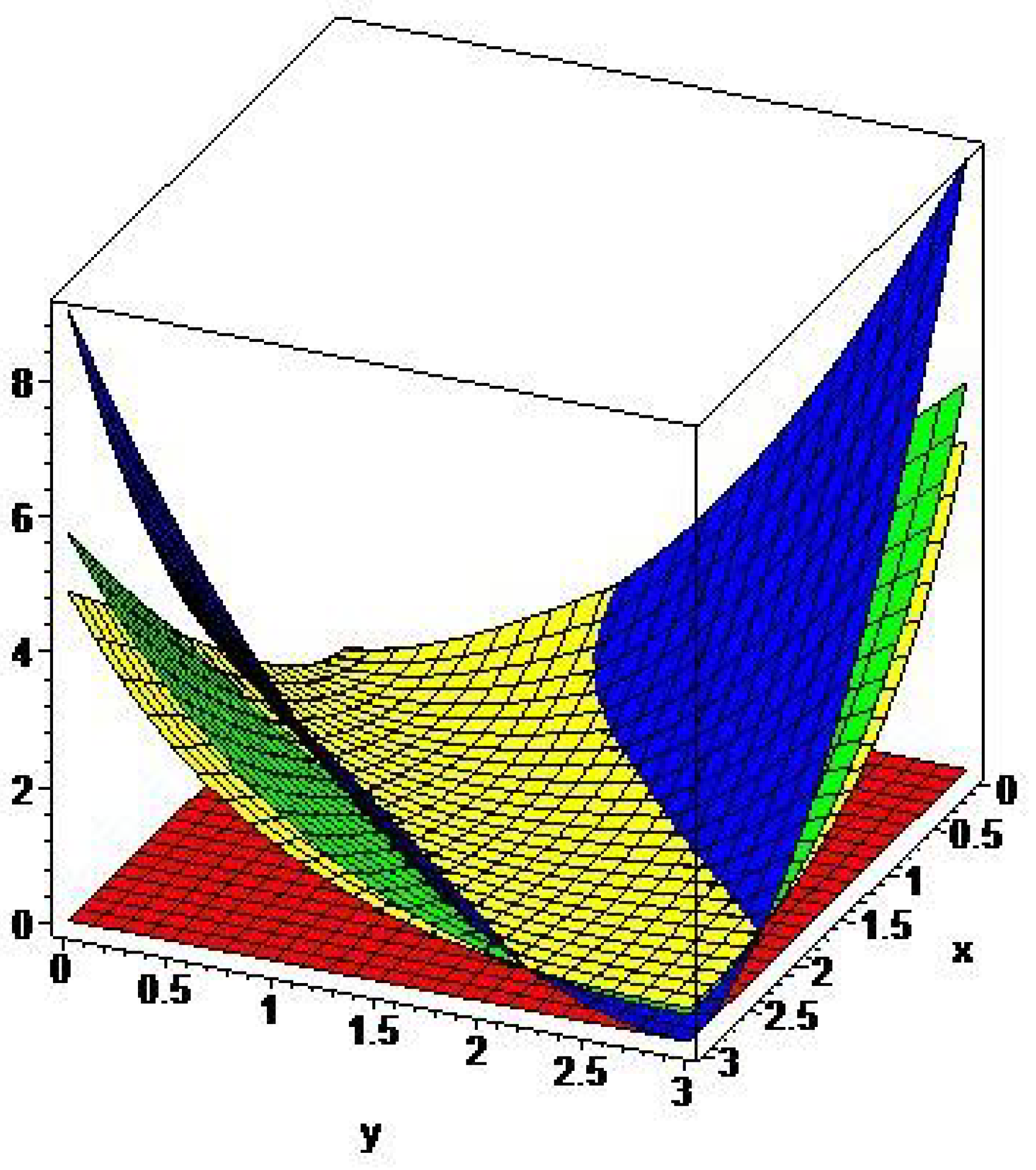
Figure 1. Approximation of R n , n G φ to φ (blue) on 0 , 3 × 0 , 3 for n = 5 (red), n = 25 (yellow), n = 75 (green).
Mathematics 10 01418 g001
Figure 2. Approximation of B n , n G φ to φ (blue) on 0 , 3 × 0 , 3 for n = 5 (red), n = 25 (yellow), n = 75 (green).
Mathematics 10 01418 g002
Figure 3. Comparison by Approximation of R 75 , 75 G φ to φ (blue) on 0 , 3 × 0 , 3 for β 1 = 1 5 n 1 (red), β 2 = 1 10 n 1 (yellow) and β 3 = 1 15 n 1 (green).
Mathematics 10 01418 g003
Figure 4. Comparison by Approximation of B 75 , 75 G φ to φ (blue) on 0 , 3 × 0 , 3 for β 1 = 1 5 n 1 (red), β 2 = 1 10 n 1 (yellow) and β 3 = 1 15 n 1 (green).
Mathematics 10 01418 g004
Figure 5. Comparison by Approximation of R 75 , 75 φ (green), R 75 , 75 G φ (red) and B 75 , 75 G φ (yellow) to φ (blue) on 0 , 3 × 0 , 3 .
Mathematics 10 01418 g005
Publisher’s Note: MDPI stays neutral with regard to jurisdictional claims in published maps and institutional affiliations.