1. Introduction
Software development management is required to optimize efficiency due to the cost of testing efforts in detecting and correcting several faults during the testing process. Therefore, evaluating testing efficiency is important both during and after the project to get feedback. One way to get useful feedback is to analyze the data collected in current and past projects. Fault-counting data are a typical data set collected in the actual testing process, with records of only the total faults during the testing period, hourly, daily, or monthly. It is used to quantitatively evaluate the final quality and reliability of software products. However, the detection and correction times of each fault are not recorded.
In large-scale software and open source software development, bug tracking systems are introduced, and various data including fault detection and correction completion times can be easily collected. However, fault-counting data are recorded using a company-specific format without introducing the bug tracking system in small- or medium-scale software development. In the latter case, it is difficult to collect data, such as fault detection and correction times, due to the cost of personnel and data collection time. Therefore, we obtain new knowledge as feedback by analyzing existing fault-counting data.
Generally, when evaluating software reliability using the fault-counting data, nonhomogeneous Poisson process (NHPP) models, which have high practicality due to their model structure, are used among the software reliability growth models (SRGMs) [
1,
2,
3]. In previous studies, the delayed S-shaped (DSS) SRGM, incorporated in two stages of software failure occurrence and fault isolation processes, was developed [
3,
4]. Additionally, new SRGMs, using the concept of separating the fault detection process, expressed the physical aspect of the fault detection process using the infinite server queuing model [
4,
5]. However, these proposed models cannot be used to evaluate the efficiency of fault correction activities because SRGMs, including NHPP models, express only the software failure/fault detection process, and cannot express a series of processes from the failure/fault occurrence to fault correction completion.
For example, the intensity function of NHPP models, which indicates the instantaneous fault detection rate, can estimate when most faults were detected. Knowing the peak time for fault detection helps plan future testing phases. However, estimating the busiest correction time and considering appropriate measures to eliminate the delay are factors that improve the efficiency of fault correction activities. Therefore, it is necessary to visualize fault correction activities. Equally, the software development manager needs to understand the status of fault correction activities.
In this paper, we generated the sample data of the fault detection time from the actual fault-counting data to conduct the efficiency evaluation of the fault correction activities. Next, we estimated the detection time of each fault using the thinning method [
6]. Then, we applied the DSS and ISS intensity functions. Furthermore, the process from fault detection to correction completion was represented by the infinite server queuing model. Visualizing the temporal behavior of the faults being corrected in the testing phase reveals the peak time when the fault correction activities are the busiest.
2. Software Reliability Growth Model
Now, let
(
) denote a counting process representing the total faults detected up to the testing time
t. Assumed
follows an NHPP, the stochastic behavior of
is given by
where
is the mean value function of NHPP and represents the expected cumulative number of faults detected in the time-interval
.
is the intensity function, indicating the instantaneous fault detection rate at time
t. When the intensity function is constant at time
t,
follows the homogeneous Poisson process (HPP). The instantaneous fault detection rate and mean value function of HPP are defined by the following equations:
In NHPP models with a finite number of detectable faults, the number of faults detected per unit time is assumed to be proportional to the number of remaining faults in the software at that time and is given by the following differential equation:
where
a is the initial fault content and
is the fault detection rate at time
t.
First, assuming that the initial conditions of Equation (
5) are
and
, the exponential (EXP) SRGM [
1,
2,
3,
7] is derived as
Suppose
and
, the following differential equation is obtained.
Solving Equation (
7) under Equation (
12), the DSS SRGM [
1,
2,
3] is derived as
Thus, the intensity function of DSS SRGM is as follows:
Next, the fault detection rate is assumed as follows:
where
l is the inflection coefficient for the fault detection ability. From Equations (
5) and (
10), the ISS SRGM [
1,
2,
3] is derived as
where
. The intensity function of ISS SRGM is as follows:
3. Sample Data Generation of Fault Detection Time Using the Thinning Method
3.1. Thinning Method
The thinning method [
6] is a sampling method that extended the rejection sampling method. It is used when random numbers cannot be directly obtained from the probability density function. Here, we simulated NHPP using the intensity function
to generate the sample data of the fault detection time. The conceptual figure of the thinning method is shown in
Figure 1.
The procedure is as follows: First, the maximum value of the intensity function of NHPP is set to . Furthermore, we generate an exponential random number, , according to HPP as a candidate for the fault detection time. Next, we generate a uniform random number on and simulate the coordinate of the candidate point . The candidate points in the upper region of the intensity function are rejected, and those in the lower region are adopted. Note that candidate points are adopted if . Each adopted time candidate point is used as the sample data of the fault detection time.
3.2. Sample Data Generation of Fault Detection Time
To determine the intensity functions, we estimated parameters of SRGMs using the following fault-counting data [
8,
9] observed in the actual testing process.
In the above data,
and
are the calendar time and total detected faults, respectively. In this study, the DSS and ISS SRGMs were applied since the above fault-counting data are an S-shaped reliability growth curve data. The estimated values
,
, and
of the parameters
a,
b, and
l included in the DSS and ISS SRGMs are estimated using the maximum likelihood method. Furthermore, mean squared errors (MSE) were used as assessment criteria for the goodness-of-fit comparison. Here, MSE is defined as
where
K is the total number of data,
is the actual value, and
is the estimated value of the cumulative number of faults.
Figure 2 and
Figure 3 are the estimated DSS and ISS SRGMs.
Table 1 presents the results of the parameter estimation and MSE. From the result of the goodness-of-fit comparison for DSS and ISS SRGMs, we observe that the ISS SRGM has better performance. The intensity functions estimated above were used to generate sample data of the fault detection time.
Figure 4 and
Figure 5 show each piece of generated data using the thinning method, and each intensity function of the DSS and the ISS SRGMs. These data were called “DSS data” and “ISS data”, respectively.
4. Queuing Simulation Using Sample Data of Fault Detection Time
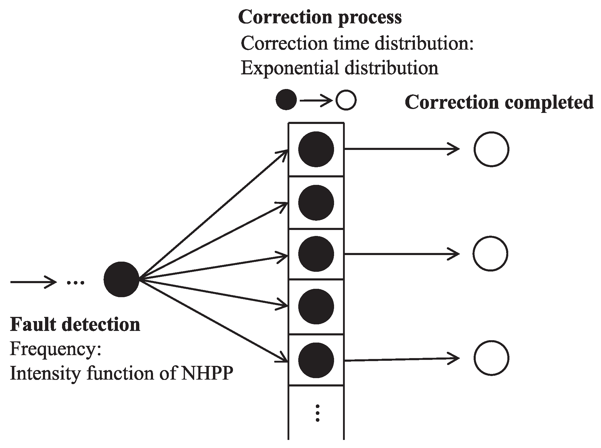
The infinite server queuing model is used for simulating fault correction activities. Detected faults enter the infinite server and the exit server when the correction is complete, as shown in
Figure 6. Suppose that the
n-th fault detection and correction times are represented by
and
, respectively, the correction completion time
is defined as the following equation:
The number of faults corrected is obtained by counting the number of faults n which fills with arbitrary time t. Assuming that the correction time follows the exponential distribution, we clarify the busy fault correction activities from the fault detection to correction completion using the queuing simulation.
Figure 7 shows the simulation result, assuming that the fault correction time follows the exponential distribution with an average of 0.5 days. Observe that the fault correction activities became the busiest around the 11th and 18th day, respectively.
Figure 8 shows the simulation result, assuming that the fault correction time follows the exponential distribution with an average of 1 day. Here, the number of faults being corrected doubled. From
Figure 7 and
Figure 8, no significant difference exists between the most fault detection time and the busiest fault correction time at the first peak. However, there is a large time difference at the second peak.
Figure 9 shows the simulation result, assuming that the fault correction time follows the exponential distribution with an average of 0.5 days. Here, the fault correction activities became the busiest around the 12th and 17th day, respectively.
Figure 10 shows the simulation result assuming that the fault correction time follows the exponential distribution with an average of 1 day.
Figure 9 and
Figure 10 show that fault correction activities are busy in the first peak due to factors such as the difficulty of detecting or correcting faults, rather than the number of detected faults.
From the above, it clear that the fault correction activities became the busiest at the time slightly different from when the fault was most detected. Additionally, model selection must be according to the goodness-of-fit and characteristics of the model because of the changing behavior of the intensity function.
5. Conclusions
In this paper, we discussed a method for evaluating the efficiency of fault correction activities in a testing phase. The sample data of fault detection time were generated to obtain new development management knowledge from existing fault-counting data. The DSS and ISS SRGMs were adopted from the behavior of the actual data, and the parameters of each model were estimated using the maximum likelihood method. The intensity functions of the DSS and ISS SRGMs were determined from the estimated parameters, and the sample data were generated using the thinning method. Furthermore, we performed a simulation using the infinite server queuing model to quantitatively evaluate the efficiency of fault correction activities. Specifically, assuming that the correction time follows the exponential distribution, the time behavior of the number of faults being corrected was presented. Therefore, we obtained that there were time lags between the peaks for the number of fault detection and correction, respectively. As a future study, it is necessary to perform the simulation using the queuing models that can express the actual testing process more and confirm their effectiveness.
Author Contributions
Conceptualization, Y.M. (Yuka Minamino); methodology, Y.M. (Yuka Minamino), S.I.; programming, Y.M. (Yuka Minamino) and Y.M. (Yusuke Makita); validation, Y.M. (Yuka Minamino) and Y.M. (Yusuke Makita); investigation, Y.M. (Yuka Minamino) and Y.M. (Yusuke Makita); resources, S.I. and S.Y.; data curation, S.I.; writing—original draft preparation, Y.M. (Yuka Minamino) and Y.M. (Yusuke Makita); writing—review and editing, S.I. and S.Y.; visualization, Y.M. (Yuka Minamino) and Y.M. (Yusuke Makita); supervision, S.I. and S.Y.; project administration, Y.M. (Yuka Minamino); funding acquisition, Y.M. (Yuka Minamino). All authors have read and agreed to the published version of the manuscript.
Funding
This work was supported by JSPS KAKENHI Grant Number 20K14983.
Institutional Review Board Statement
Not applicable.
Informed Consent Statement
Not applicable.
Data Availability Statement
Not applicable.
Conflicts of Interest
The authors declare no conflict of interest.
References
- Pham, H. System Software Reliability; Springer: London, UK, 2006. [Google Scholar]
- Zhu, M.; Pham, H. Software reliability modeling and methods: A state of the art review. In Optimization Models in Software Reliability; Aggarwal, A.G., Tandon, A., Pham, H., Eds.; Springer: Cham, Switzerland, 2022; pp. 1–29. [Google Scholar]
- Yamada, S. Software Reliability Modeling—Fundamentals and Applications; Springer: Tokyo, Japan; Heidelberg, Germany, 2014. [Google Scholar]
- Kapur, P.K.; Aggarwal, A.G.; Anand, S. A new insight into software reliability growth modeling. Int. J. Perform. Eng. 2009, 5, 267–274. [Google Scholar]
- Kapur, P.K.; Anand, S.; Inoue, S.; Yamada, S. A unified approach for developing software reliability growth model using infinite server queueimg model. Int. J. Reliab. Qual. Saf. Eng. 2010, 17, 401–424. [Google Scholar] [CrossRef]
- Omi, T.; Nomura, S. Time Series Analysis for Point Processes; Kyoritsu-Publication: Tokyo, Japan, 2019. (In Japanese) [Google Scholar]
- Kazuhira, O. An overview practical software reliability prediction. In Reliability Modeling with Computer and Maintenance Applications; Nakamura, S., Qian, C.H., Nakagawa, T., Eds.; World Scientific: Singapore, 2017; pp. 3–21. [Google Scholar]
- Zhang, X.; Pham, H. Comparisons of nonhomogeneous Poisson process software reliability models and its applications. Int. J. Syst. Sci. 2000, 31, 1115–1123. [Google Scholar] [CrossRef]
- Tohma, Y.; Yamano, H.; Ohba, M.; Jacoby, R. The estimation of parameters of the hypergeometric distribution and its application to the software reliability growth model. IEEE Trans. Softw. Eng. 1991, 17, 483–489. [Google Scholar] [CrossRef]
| Publisher’s Note: MDPI stays neutral with regard to jurisdictional claims in published maps and institutional affiliations. |
© 2022 by the authors. Licensee MDPI, Basel, Switzerland. This article is an open access article distributed under the terms and conditions of the Creative Commons Attribution (CC BY) license (https://creativecommons.org/licenses/by/4.0/).


