In this section, numerical results are given to illustrate the accuracy and efficiency of the method we propose.
5.1.
When , the problem simplifies to determining the finite-time survival probabilities. Next, the performance of the DNN approach in solving for the finite-time survival probabilities under the classical risk model is demonstrated. For the following examples with different claim size distributions, we use two sets of network parameters to obtain the numerical results:
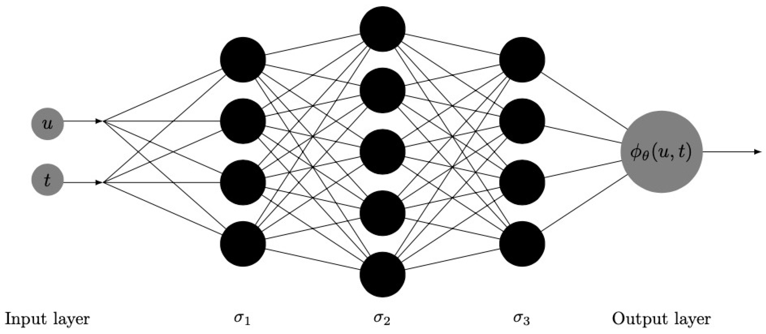
Parameter 1: 4 hidden layers, each layer has 8 neurons, the activation function is the tanh function, and the times of training is 50,000;
Parameter 2: 10 hidden layers, each layer has 20 neurons, the activation function is the tanh function, and the times of training is 50,000.
In order to ensure the accuracy of parameter convergence and improve the speed of parameter updating iteration, we adopt a piecewise learning rate instead of a fixed learning rate with
where
represents the learning rate of the gradient descent type algorithm, and the learning rate for the first 1000 iterations is 0.01. From 1000 to 3000 iterations, the learning rate is 0.001; for all iteration steps after the 3000th iteration,
. It decays in a piecewise constant and establishes a ’tf.keras.Optimizer’ to train the model.
Example 1. Considering the classical risk model as described in Equation (1), we assume that the individual claim sizes are exponentially distributed with parameter , the premium income is , and the parameter of the Poisson process is . Firstly, the training data set is constructed. Setting , we randomly select 200 data points according to uniform distribution in the region and then select 30 points on the initial value , that is, , .
Figure 3 demonstrates the training data selected according to uniform distribution in a given area. For the initial value data point, that is,
, we select
u according to the equidistance principle. In the figure, the mark ’x’ is used to represent the data points selected at the initial time
. The data points in the region are randomly sampled and represented by gray points. In addition, data points on the boundary can also be added in the construction of the training data set, which can make the neural network training results more accurate.
Figure 4 shows the finite-time survival probability calculated by the DNN approximation method after 50,000 iterative calculations, and when using Simpson’s rule to process the integral term, we set
. From the image of the numerical solution, we know that the approximate solution obtained by the deep neural network method is consistent with our expected results.
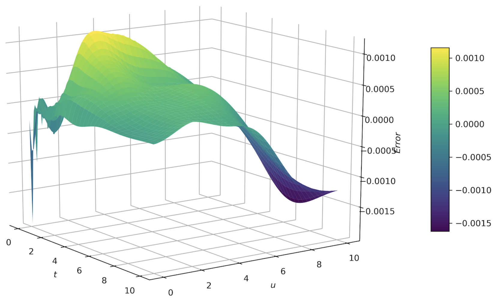
Figure 5 and
Figure 6 show the errors between the approximate solutions and exact solutions after 50,000 times of training of two groups of different neural network parameters. We can see that under Parameter 1, the errors between the value calculated by DNN method after 50,000 times of training and the exact solution range from 0 to 0.0015; under Parameter 2, the error range is roughly between 0 and 0.001. On the whole, the error in
Figure 6 is smaller. Combined with the results in
Figure 5 and
Figure 6, and
Table 1, we can see that the more layers there are in the neural network and the higher the number of neurons in each layer, the more accurate the calculation results are. However, the more complex the network structure is, the more resources are consumed in the calculation. Therefore, in order to balance the accuracy of the calculation results, the time needed for program calculation, and the computational resources consumed, a more appropriate set of parameters needs to be selected, which usually requires the experimenter to have enough experience.
The key points of
Table 1 are as follows:
- (1)
gives the exact values of the finite-time survival probabilities;
- (2)
denotes the values of the survival probabilities computed by using the multinomial lattice approximate method proposed by [
15] with
;
- (3)
represents the values calculated by the Monte Carlo simulation with 10,000 path and ;
- (4)
represents the values calculated by the nonparametric estimation (see [
21]) with 10,000 data points;
- (5)
denotes the values computed by using the DNN method with parameter 1;
- (6)
denotes the values computed by using the DNN method with parameter 2.
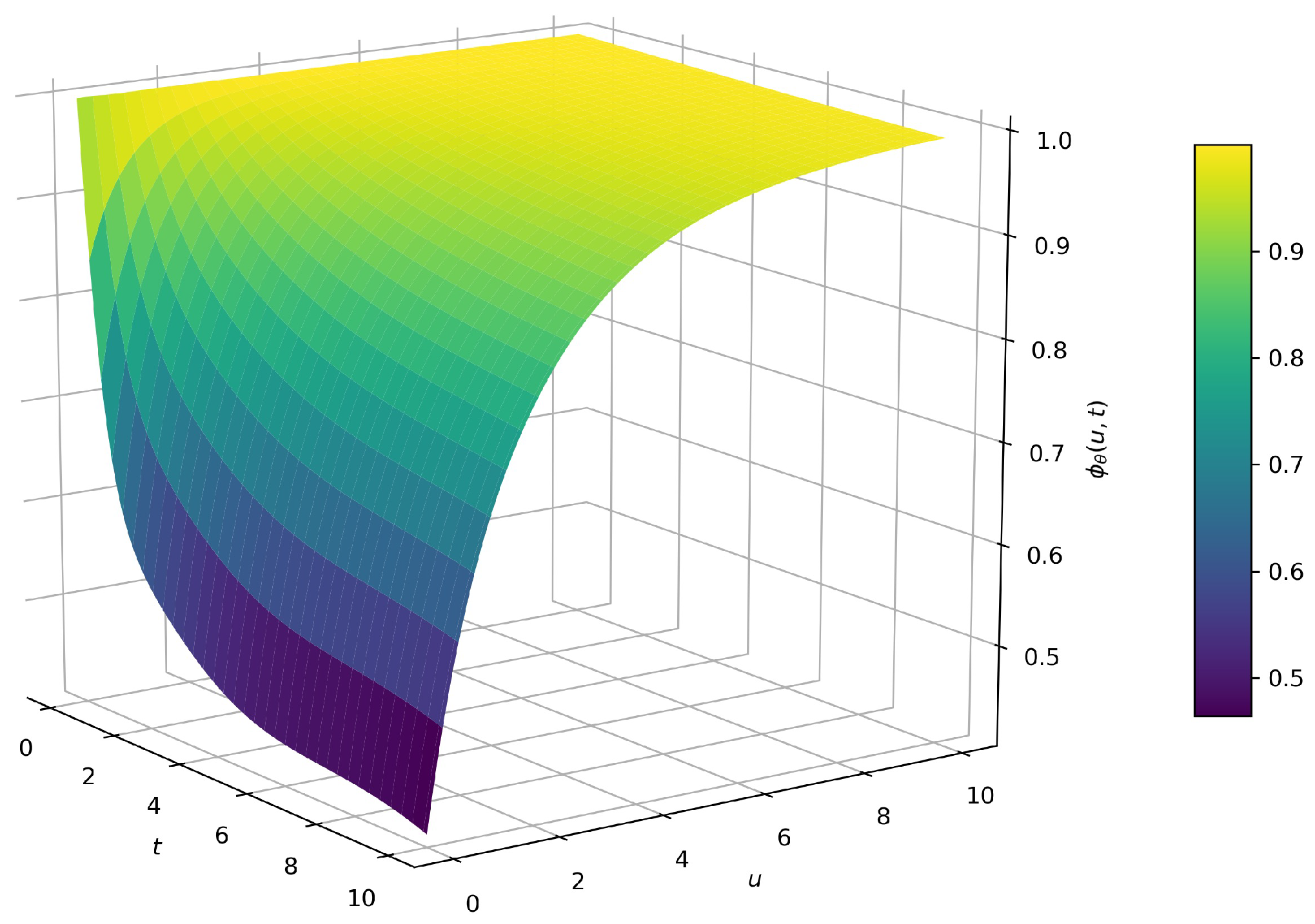
Example 2. Considering the classical risk model as described in Equation (1), we assume that the individual claim size follows Pareto distribution with parameter , the premium income is , and the parameter of the Poisson process is . Figure 7 shows the approximations of survival probability calculated by the DNN method when the individual claim function is a Pareto distribution. It can be seen from the figures that when
t is fixed, the probability of survival increases when the initial surplus level
u increases, and when
u is fixed, the probability of survival decreases as
t increases.
The key points of
Table 2 are as follows:
- (1)
denotes the values of the survival probabilities computed by using the multinomial lattice approximate method with ;
- (2)
represents the values calculated by the Monte Carlo simulation with 10,000 path and ;
- (3)
represents the values calculated by the nonparametric estimation with 10,000 data points;
- (4)
denotes the values computed by using the DNN method with parameter 1;
- (5)
denotes the values computed by using the DNN method with parameter 2.
5.2.
When
, the problem becomes how to find the joint distribution function (df) of the ruin time and the deficit at ruin. The joint df satisfies the equation,
Then, we use DNN method to solve Equation (
28) under the classical risk model. For the following examples with different claim size distributions, we use a network architecture as follows: 4 hidden layers, each layer has 8 neurons, and the activation function is the tanh function. In order to ensure the accuracy of parameter convergence and improve the speed of parameter updating iteration, we adopt a piecewise learning rate instead of a fixed learning rate
where
means that for the step size in the gradient descent type algorithm, the first 1000 steps use a learning rate of 0.01; from 1000 to 3000 the learning rate = 0.001; from 3000 onward, the learning rate = 0.0005, which decays in a piecewise constant fashion, and we set up a “tf.keras.optimizer” to train the model.
Example 3. We assume that individual claims follow an exponential distribution with the same parameters as Example 1.
Example 4. We assume that individual claims follow a Pareto distribution with the same parameters as Example 2.
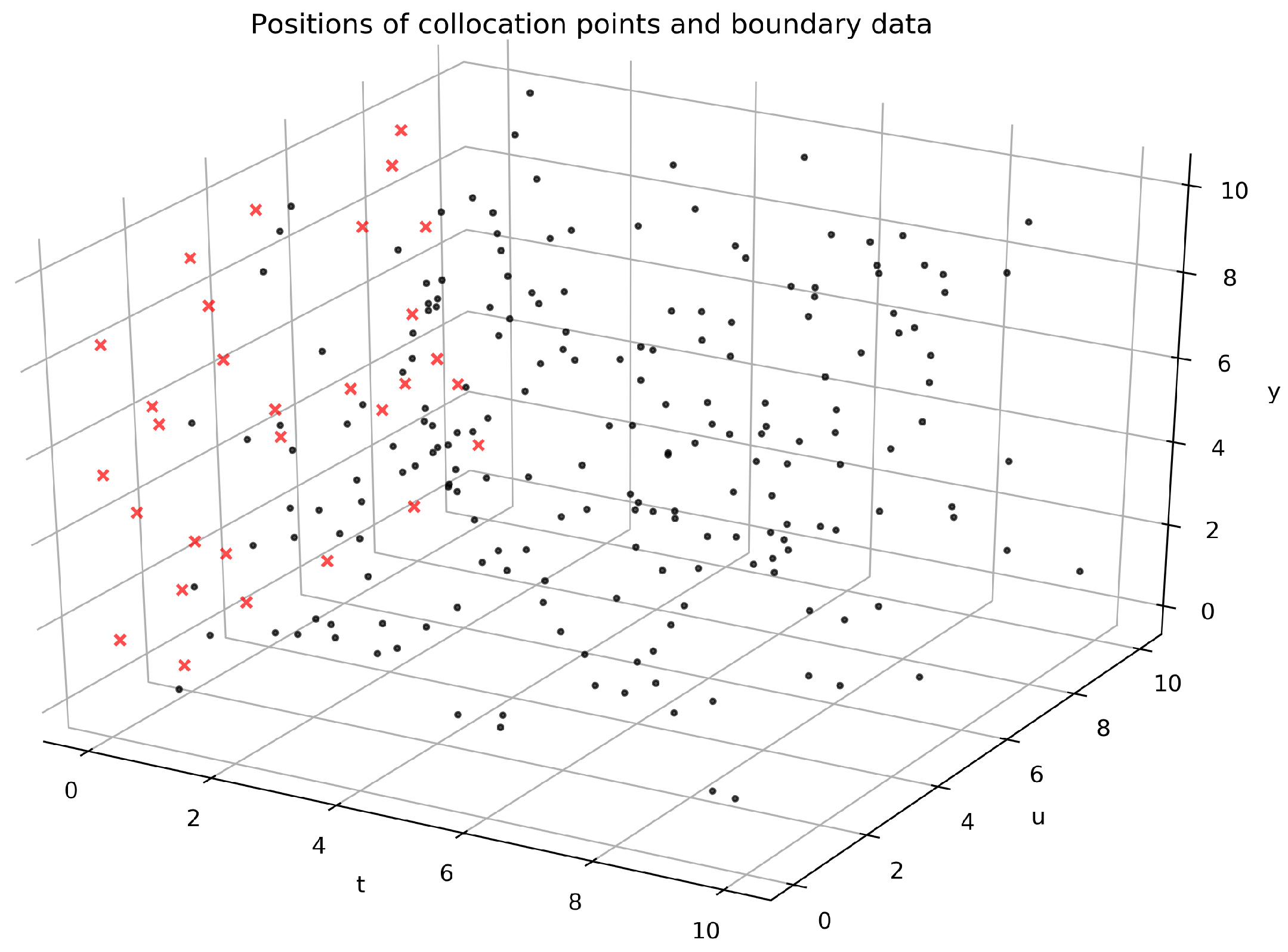
Firstly, the training data set is constructed and letting
, we randomly select 200 data points according to uniform distribution in the region and then select 30 points on the initial value
, that is,
,
. The data collected to construct the training data set for solving Equation (
28) are shown in
Figure 8. The data points at
are represented by a red ’x’, and the data samples inside the region are represented by black dots. All data points are randomly sampled.
Figure 9,
Figure 10 and
Figure 11 are the numerical simulation results of Example 3, and
Figure 12,
Figure 13 and
Figure 14 are the results of Example 4.
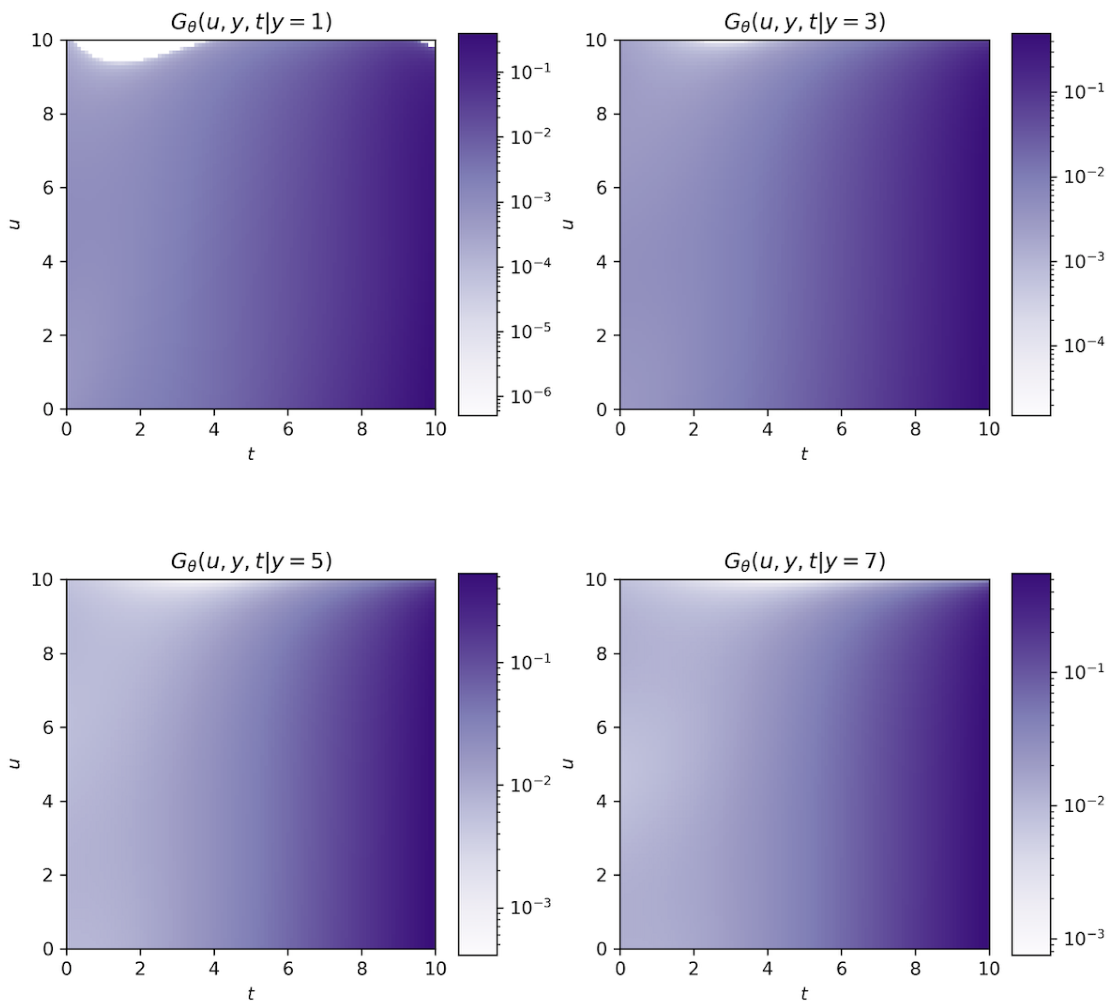
Figure 9 is the approximate solution obtained when
y is fixed. We know that as
y goes to infinity,
degenerates into the distribution of ruin time. Therefore, if
y and
u are constant, the value of
should increase as
t increases; if
y and
t are fixed, the value of
decreases as
u increases. This is consistent with the numerical simulation results in
Figure 9; with the increase in
y or
t, the color in the region gradually deepens, which means that the value of the joint distribution
keeps increasing.
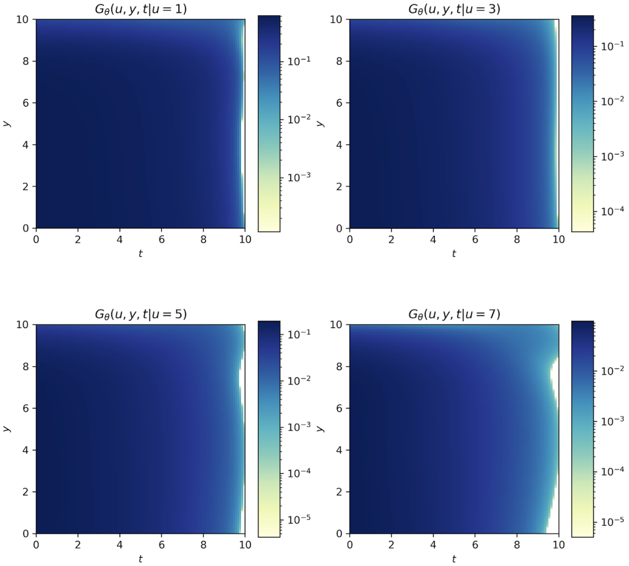
Figure 10 shows the numerical solution when
t is fixed. As can be seen from the four subgraphs from the top left to the bottom right, under the condition that
u and
y remain unchanged, the overall color of the figures are deepened with the increase in
t, that is, the numerical result of
becomes larger with the increase in time. This is the same as the theory that the longer the period of time, the greater the probability of bankruptcy, and when
, the ruin probability is 0. With other things being equal, the smaller the amount of initial capital, the greater the ruin probability. The numerical results given in
Figure 11 also confirm the fact that as
u increases, the value of
decreases. In other words, as
u increases, the color in the region gradually becomes lighter, that is, the corresponding joint distribution value also decreases.
In
Figure 12,
Figure 13 and
Figure 14, we use the DNN method to give numerical solutions of the joint distribution of ruin time and the deficit at ruin
with a Pareto claim distribution.
Figure 12 shows that with the increase in
t, the value of
also increases, that is, the longer the time, the greater the ruin probability. This result is similar to that of the exponential distribution; moreover, the results shown in
Figure 13 and
Figure 14 are the same as those obtained for the exponential claim size (
Figure 10 and
Figure 11). According to the results in
Figure 9,
Figure 10 and
Figure 11, we can see that deep learning is also suitable for solving high-dimensional problems. After setting an appropriate network structure, more accurate results can also be obtained after repeated network training.
It can be seen from the results in
Table 3 and
Table 4 that the calculation time consumed by the deep neural network in training data sets is positively correlated with the total number of training times. When Simpson’s discretization is used to deal with the integral term, the calculation time is greater, and if the replacement formula is used, the calculation time is greatly reduced.
Table 5 shows the CPU time of the Monte Carlo method under different path number settings when
and
. It is worth mentioning that the results obtained by the DNN method are not for a single data point
; rather, for a given whole interval
, the plane of the numerical solution is given. The Monte Carlo method and other approximate algorithms can only solve a single data point
. Based on its calculation efficiency, it can be seen that the DNN method has great advantages.
Moreover, the DNN method has another significant advantage: it does not consume much computer storage space. Random simulation and other approximation algorithms need to split the direction of time and space in the calculation process, so the previous results need to be stored in each calculation, that is, the finer the grid, the greater the required computer storage space. However, the deep neural network method updates the parameters according to each calculation result, that is, there is no need to store all the calculation results, thus greatly reducing the consumption of computer memory resources.


