Abstract
In recent years, technologies for renewable energy utilization have been booming. Hybrid renewable energy systems (HRESs), integrating multiple energy sources to mitigate the unstable, unpredictable, and intermittent characteristics of a single renewable energy source, have become increasingly popular. However, due to the inherent intermittency and uncertainty of renewable energies, the impact of uncertain factors on the capacity optimization of HRESs needs to be considered. In the traditional scenario-based planning method, when dealing with uncertain factors, the probability corresponding to the scenario is difficult to determine. Furthermore, when applying the robust optimization method, it is difficult to fully use existing data to describe uncertain parameters in the form of intervals. To tackle these difficulties, this study proposes a probability undetermined scenario-based sizing model (PUSS model) for stand-alone HRES configuration optimization and a multi-objective evolutionary algorithm as the problem solver. The solution set obtained by the method covers multiple possible values of scenario probability combinations and can provide decision-makers with an overview of alternatives for HRES sizing under different power supply pressures. Based on the real environment data and load data of a certain place, the proposed model and algorithm are applied to sizing a typical HRES comprising wind generators, solar photovoltaic panels, energy-storage devices, and diesel generators. The experimental results show that the proposed PUSS method is both effective and efficient.
Keywords:
HRES; microgrid; multiple scenarios; multi-objective optimization; evolutionary algorithms; decision-making MSC:
90C29
1. Introduction
As countries continue to focus on energy security and the need to achieve low-carbon development, more and more hybrid renewable energy systems (HRESs) have been built and put into practice. Because of its multi-energy complementarity and its ability to operate off-grid, a self-sufficient, independent hybrid renewable energy system is often used for power supply on remote islands and in high mountain residential areas. Simultaneously, the structure of microgrids can be adjusted to meet specific local needs.
Till now, researchers have conducted a series of relevant research for the optimal design of microgrids [1,2,3]. The data, e.g., solar radiation intensity or wind speed, is often taken from historical records [1,2] or is predicated based on historical data [3]. Even if different types of neural networks are used for prediction, the application scenarios are different [4,5,6], and the predicted results still reflect the characteristics of historical data. However, due to the inherent intermittency and uncertainty of the output of renewable energies, even if multi-energy complementarity [1,2,3] is achieved, its energy supply still has many unstable factors than traditional hydropower and thermal power plants. When climate anomalies or natural disasters occur, this intermittency and uncertainty can even become extremely deadly. Therefore, in the capacity optimization of HRESs, the influence of uncertain factors needs to be considered.
Using the existing methods considering uncertainty [7,8,9,10,11,12,13,14,15,16,17] to perform microgrid planning can only obtain a set of solutions with a certain degree of environmental uncertainty. Hence, decision-makers can only choose among the solutions with this degree of uncertainty. To solve these problems, this paper proposes a probability undetermined scenario-based sizing model (PUSS model) for HRES configuration optimization. We incorporate the occurrence probability of the scenario into the optimization objectives. A set of configuration schemes that can cope with various environmental uncertainties can be obtained by conducting the proposed multi-objective evolutionary algorithm. This solution set allows decision-makers to intuitively understand the relationship between the maximum environmental uncertainty that the microgrid can bear and the objectives (for example, economic costs, lost probability of power supply, etc.) of configuration optimization. The PUSS model does not rely on the probability distribution of various uncertain factors and does not need to obtain the probability of each uncertain scenario. Multiple solutions that are used to deal with different environmental data uncertainties can be obtained in a single run.
The contributions of this paper are summarized as follows:
(i) A probability undetermined scenario-based HRES sizing (PUSS) model is proposed. This model can solve the issue that traditional scenario-based HRES configuration optimization relies heavily on actual data or cannot make full use of existing data.
(ii) The effectiveness of the PUSS model is demonstrated by comparing its results with those obtained by repeatedly solving the scenario-based dual-objective HRES optimization with preset scenario probability combinations. PUSS obtains a comparable solution quality, but with significantly less calculation cost.
The remainder of this paper is organized as follows: Section 2 reviews related studies for microgrid planning considering uncertainty. Section 3 introduces the structure, main energy supply unit model, and operation strategy of HRESs. Section 4 elaborates the principles of the PUSS model and its application. In Section 5, the solution of the PUSS model is performed based on NSGA-II, whose results are compared with the results of a scenario-based dual-objective HRES optimization method using the same algorithm, NSGA-II. Section 6 concludes this study.
2. Literature Review
In the literature, there are mainly two classes of methods to deal with uncertainties in HRES configuration optimization. These are robust optimization methods and stochastic programming.
HERS configuration optimization based on robust optimization generally uses the interval form to describe uncertain factors such as wind speed and illumination intensity. The authors in [10] adopted a robust optimization method to perform energy system design and found that the obtained results exhibit better performance than those obtained by a deterministic model. The study [11] considered the trade-off between expected costs in the nominal scenario and costs in the worst case while guaranteeing the security of energy supply. A two-stage robustness trade-off approach was proposed to design energy supply systems.
Robust optimization methods based on uncertain parameters described in the form of intervals require fewer characteristics of the uncertain parameters. Only the fluctuation interval instead of the accurate probability distribution is required, which makes the robust optimization method widely used in engineering problems [10,11,13,15]. However, at the same time, it brings about the problem that too little information is needed and the existing information cannot be effectively used when using a robust optimization method to perform HRES configuration optimization. This makes robust optimization methods bring large additional costs while ensuring energy supply security.
In terms of stochastic programming, a typical way is to use multiple scenarios to represent the relevant uncertainty and set each scenario with a corresponding probability. The work [7] presented a model for optimal distributed energy system design under uncertainty, which was formulated as a two-stage stochastic mixed-integer linear program, and probabilistic scenarios were used to describe the uncertainty. In [8], a stochastic model was proposed for coordinated scheduling of renewable and thermal units. Uncertainties of wind speed, solar irradiation, and market prices were considered in this scenario-based model. In [9], a scenario-based method was used for modeling the uncertainties of electrical market price, wind speed, and solar irradiation, and the multi-objective firefly algorithm was used to solve the stochastic nonlinear programming model.
The description of uncertainty in stochastic programming methods is often based on scenarios. The scenarios and the corresponding probability of each scenario should reflect the future operation of HRESs. However, the scenario structure and the determination of the scenario probability under this requirement is quite difficult. There are many uncertain factors in the microgrid system, and the probability distribution function is complex, which is difficult to obtain accurately. Correspondingly, the reliability of the optimization results obtained by the stochastic optimization method is weakened.
Besides, there is also a class of scenario-based robust optimal design methods [16,17], which have been developed from the minimax regret criterion (MMR) method [18] and derived minimax expected criterion (MER) [19] and other methods. In [12], a new method was proposed to solve the upper bound of the maximum regret optimal value and revise the robust optimization design method of the energy supply system under uncertain energy demand. Since such methods also perform optimization calculations based on energy use scenarios and their corresponding probabilities, they all face the same issue of determining a proper probability of each scenario.
In summary, when sufficient information is available, the optimization results obtained by stochastic programming or scenario-based robust optimization methods are often better than those obtained by robust optimization methods that describe uncertain parameters in the form of intervals. However, it is not easy to construct the scenario needed for optimization and determine its corresponding probability. The above-mentioned methods used to deal with uncertain factors in HRESs have their shortcomings. For example, they can only perform optimization based on a certain degree of environmental uncertainty (indicated by uncertain intervals or scenarios with their corresponding probabilities). In this way, the optimization results are only able to deal with a specific maximum environmental uncertainty and cannot reflect the relationship between environmental uncertainty and the goals of microgrid optimization.
Compared with the traditional stochastic programming method, the PUSS model proposed in this study does not need to pre-determine the probability of each scenario. Furthermore, a variety of configuration schemes, corresponding to various maximum environmental uncertainties, can be obtained in one solution set. As for the scenario-based robust optimization method, since the PUSS model uses the same probabilistic way as the stochastic programming method in describing scenarios, rather than describing the uncertainty by uncertainty intervals, and the use of the PUSS model would generally lead to better results than interval-number-based robust optimization methods.
3. HRES Model
3.1. The Structure of the HRES
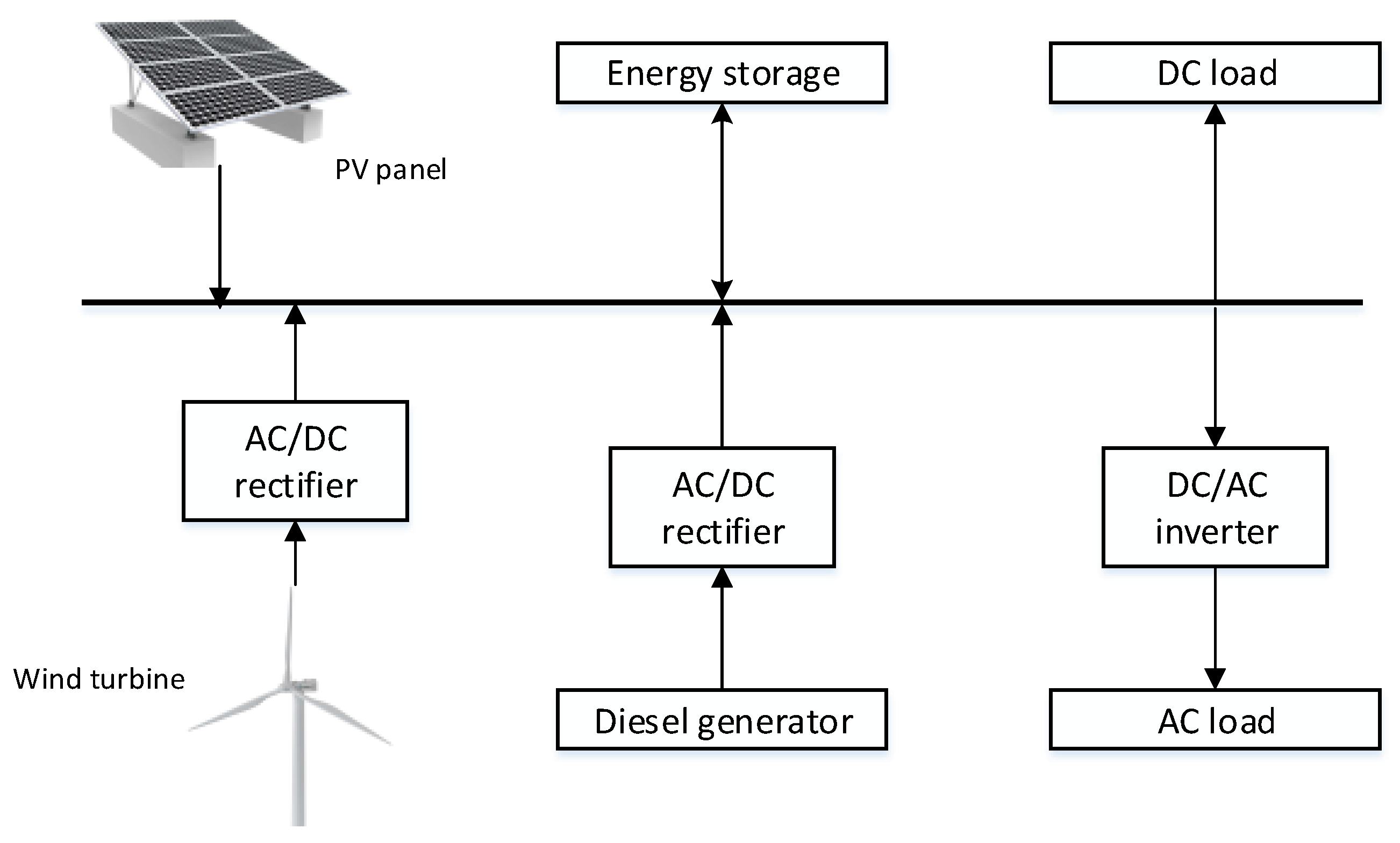
The case study in this study is based on an off-grid HRES using a DC bus structure simplified from [20], consisting of photovoltaic panels, wind turbines, diesel generators, batteries, and other accessories, as shown in Figure 1. The unit models of the system are shown in [20]. The HRES sizing involves the combinatorial optimization of multiple devices. For a certain probability combination of the scenario set, the optimal solution needs to be weighed under multiple goals to satisfy the requirements of reliable power supply, low cost, and environmental friendliness. This study, therefore, proposes a method to find an optimal solution under different probability combinations of the scenario set.
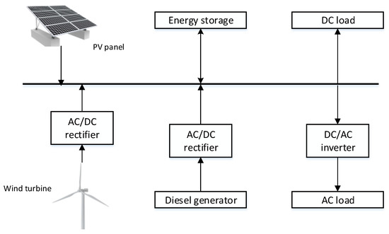
Figure 1.
Off-grid HRES structure.
3.2. HRES Operating Strategies
Since the off-grid HRES model in this paper uses a DC bus, the electrical energy output by photovoltaic arrays and wind turbines will be directly supplied to the DC loads, and it will be converted by the inverter when supplying AC loads. If the power generated by renewable energies exceeds the total demand (DC loads plus AC loads), the excess power would be stored in the battery packs after all loads are met. Conversely, if the amount of power generated by renewable energies cannot meet the load demand, the battery pack would be discharged based on the state of charge, that is the state of charge cannot be lower than the minimum.
If the battery packs can meet all loads, they will meet the DC loads and the AC loads in order; if they still cannot meet the load demand, the diesel generators start to fill the power shortage. Because the electricity generated by the diesel generators is alternating current, the electricity used to provide the DC loads will be converted into direct current by the rectifier. If the diesel generators are all running at full power output, but the microgrid system still has a power shortage, this situation will be included in the statistics of the lack of power supply.
4. PUSS Model
4.1. Principle of the Model
4.1.1. Microgrid Operating Scenario and Its Power Supply Pressure
Before introducing the PUSS model, the microgrid operating scenario (hereinafter referred to as simply the scenario) and the power supply pressure are defined. The scenario used in microgrid optimization is essentially a microgrid operating state determined by environmental conditions and load demand. Scenarios are generally generated based on actual data, and a small number of representative scenarios are obtained for microgrid optimization through clustering and some scenario reduction methods.
For a specific scenario, environmental conditions such as solar irradiation and wind speed in the scenario affect the power supply capacity of the microgrid. Whether the power supply capacity matches the load demand determines the power supply pressure of the microgrid in this scenario. Specifically, the power supply pressure of a scenario refers to the difficulty for the HRES to meet the power demand of all loads in this scenario. The more difficult it is to meet the power demand of all loads, the larger the pressure on the power supply is.
4.1.2. The Occurrence Probability of the Scenario
In the traditional scenario-based method, the occurrence probability of each scenario needs to be determined when constructing the scenario set required for optimization; the sum of the probabilities of all scenarios in the set is 1. In the PUSS model, the occurrence probabilities of the scenarios used for optimization need not be determined in advance.
The scenario set required by the PUSS model can be expressed as: . The occurrence probability corresponding to the scenario is denoted as , . Here, the label i of is determined according to the power supply pressure of the microgrid in each scenario. The smaller the power supply pressure, the smaller the label. Then, we have:
indicates the power supply pressure in scenario . The maximum power supply pressure must be strictly greater than the power supply pressure of other scenarios.
In this paper, , which corresponds to element in the scenario set, constitutes probability set P. For the set P, there are:
Here, the set obtained by assigning values to all the elements in P is defined as a scenario probability combination.
4.1.3. Optimization Objectives
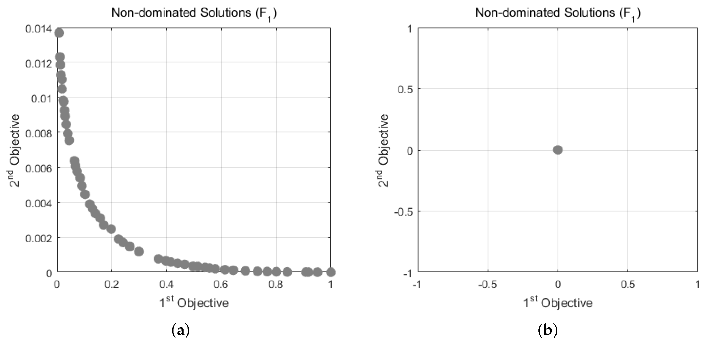
This paper proposes a probability undetermined scenario-based sizing model (PUSS model) and algorithm for off-grid HRES configuration optimization. In general, objectives in a multi-objective problem conflict with one another. Figure 2 illustrates the solution set of the inverted two-objective MOP2 problem obtained by NSGA-II.

Figure 2.
Example of a two-objective minimization problem solution set. (a) Mutually constrained dual-target Pareto front. (b) Unconstrained two-objective optimization results.
Taking the dual-target capacity optimization of the HRES as an example, the annualized cost of the system (ACS) and the loss probability of power supply (LPSP) are selected as the optimization goals. The objective function should be:
Minimizing the LPSP requires a higher power supply capacity of the microgrid, which naturally leads to an increase in the annual cost of the microgrid. Therefore, there is a restrictive relationship between the ACS and LPSP.
The ACS and LPSP are computed according to the PV power, wind power, diesel power, load power, battery charging, and discharging power. Specifically, the output power of PV panels is computed by [20]:
where are decision variables that indicate the number of PV modules and the PV panel slope angle. Refer to [20] for the details of other parameters. The output power of wind turbine is computed by [20]:
where is the decision variable that indicates the wind turbine height. is the wind speed at the reference height . are the cut-in, cut-off, and rated wind speed. In addition, the battery model is constructed as:
where represents the charging power and represents the discharging power. is the total capacity of the energy storage determined by the number of batteries , which is to be optimized. and are the DC bus voltage and the round-trip efficiency.
Accordingly, the objective of the LPSP is computed as:
where are the output power of diesel generators, PV panels, wind turbines, and batteries, as calculated above.
The ACS is computed as:
where represents the annualized cost of initial investment, which is determined by the number of diesel generators, PV panels, wind turbines, and batteries. is the operation and maintenance cost, which is calculated by the number/time of operations and fuel consumption. The fuel consumption of the diesel generator is computed as:
where are fuel consumption coefficients and represents the rated power of the generator.
The PUSS model adds all the elements in the probability set P, except (the amount of elements in P is n), to the original objective function and hopes to minimize the new objective function :
For the microgrid, the new objective function minimizes the occurrence probability of scenarios with low power supply pressure. In other words, the occurrence probability of the scenario with the highest power supply pressure is maximized. This requires that the microgrid has a higher power supply capacity; there is also a restrictive relationship between the ACS and the scenario probabilities in . Therefore, solving the PUSS model, we can obtain the required Pareto front.
At this front, each solution (configuration scheme) corresponds to a scenario probability combination. This scenario probability combination reflects the maximum environmental uncertainty that the microgrid constructed with its corresponding scheme can withstand. In the combination of scenario probabilities, the greater the occurrence probability of scenarios with high power supply pressure, the greater the maximum environmental uncertainty that the corresponding configuration scheme can withstand.
Through this Pareto front, decision-makers can intuitively understand the relationship between the maximum environmental uncertainty that the microgrid can bear and other objectives in .
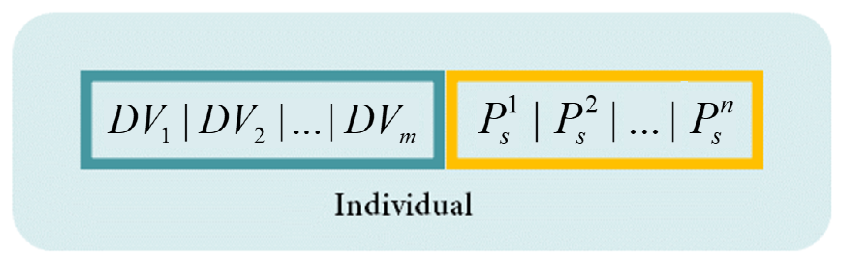
4.1.4. Encoding Individuals
At the same time, the encoding of population individuals in evolutionary computation must be adjusted accordingly. The PUSS model encodes decision variables of optimization and a randomly generated scenario probability combination into an individual. Thus, the scenario probability combinations of individuals change in the crossover and mutation process. Individual chromosome composition is shown in Figure 3. Among them, are decision variables in the optimization and are all elements in the scenario probability combination.

Figure 3.
Individual chromosome composition.
The advantage of this method is that the optimal decision variable sets corresponding to similar scenario probability combinations are often similar, and the information of the optimal solution under similar scenario probability combinations can be effectively used when searching for optimal solutions under different scenario probability combinations. In this way, the optimal solution set under a variety of different scenario probability combinations can be obtained quickly.
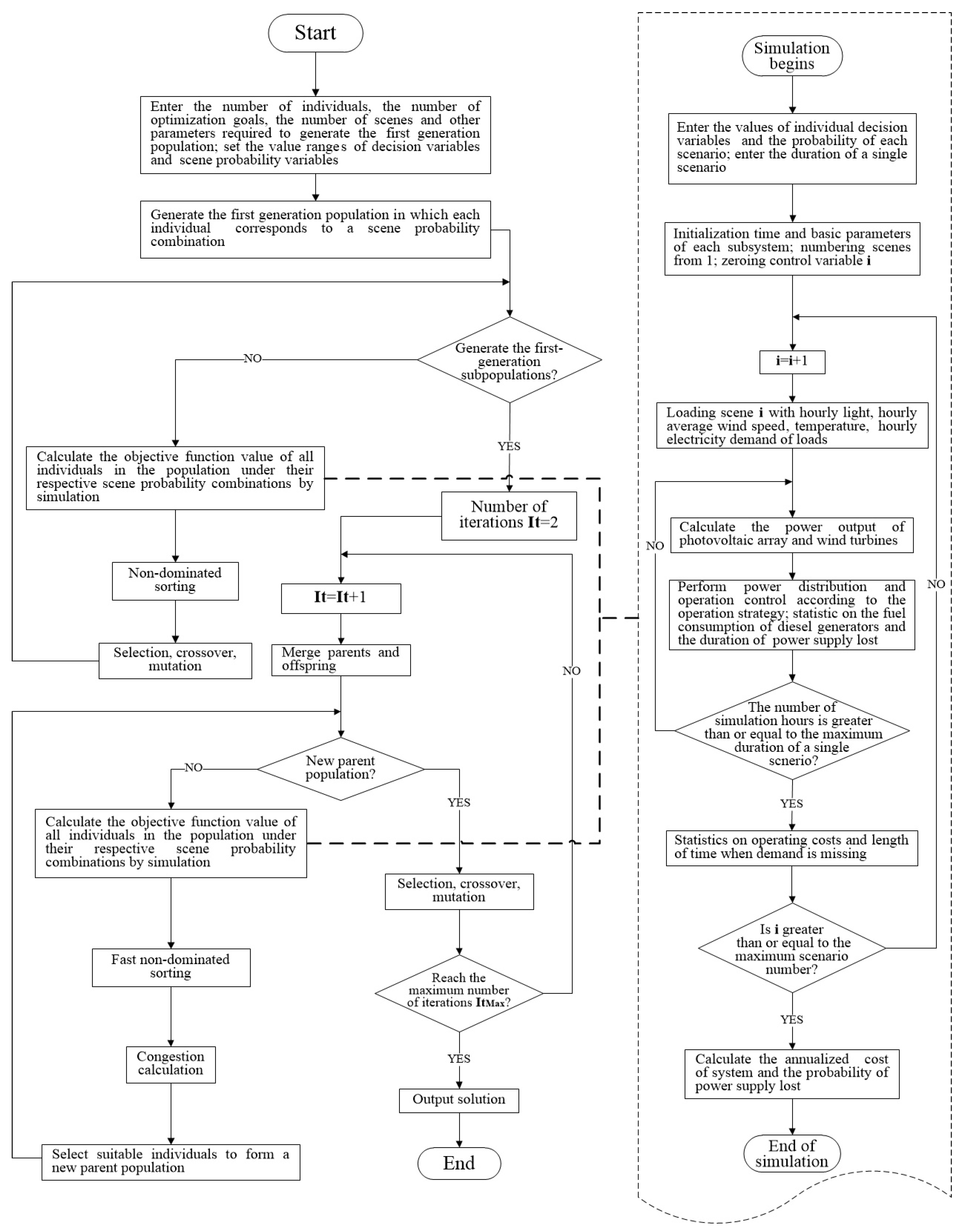
4.2. Solving Procedure
In past studies, several multi-objective evolutionary algorithms have been proposed, e.g., NSGA-II [21], SPEA2 [22], IBEA [23], MOEA/D [24], and RVEA [25]. Among them, NSGA-II [21] perhaps is the most popular one, which has been applied in many disciplines [26,27]; its characteristics are also suitable for the experiments in this study.
All the solving process in the experimental part of this paper are based on NSGA-II. When using NSGA-II, the procedure of solving the PUSS model is as shown in Figure 4.

Figure 4.
Flowchart of the PUSS model based on NSGA-II.
The input variables include the population size, the number of objectives, the total number of scenarios, the range of the decision variables, and the probability variables of the scenarios. Then, we generate the initial population and start the evolutionary computation. The objective function value is calculated by the simulation of the HRES. Since the probability combinations of the scenarios corresponding to each individual in the population are different, the probability of each scenario is used as the proportion of the total simulation duration (8760 h) in the simulation calculation. After fast non-dominated sorting, congestion calculation, selection, crossover, and mutation operations, a new generation of the population is obtained. When the evolution reaches the maximum generation, the loop is terminated and the final Pareto front is output.
5. Case Study
5.1. Data Preparation
For the purposes of validating the PUSS method, a remote region (41.65 degrees north latitude) in Spain was selected as the background to carry out the case study. The distribution of the data including load consumption, solar irradiation, temperature, and wind speed is shown in Figure 5, with a total duration of 8760 h.
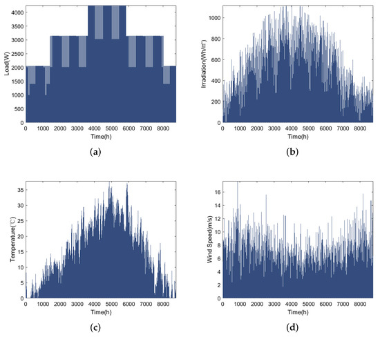
Figure 5.
Distribution of load data and environmental data. (a) Load. (b) Solar irradiation. (c) Temperature. (d) Wind speed.
5.2. Typical Scenario Construction
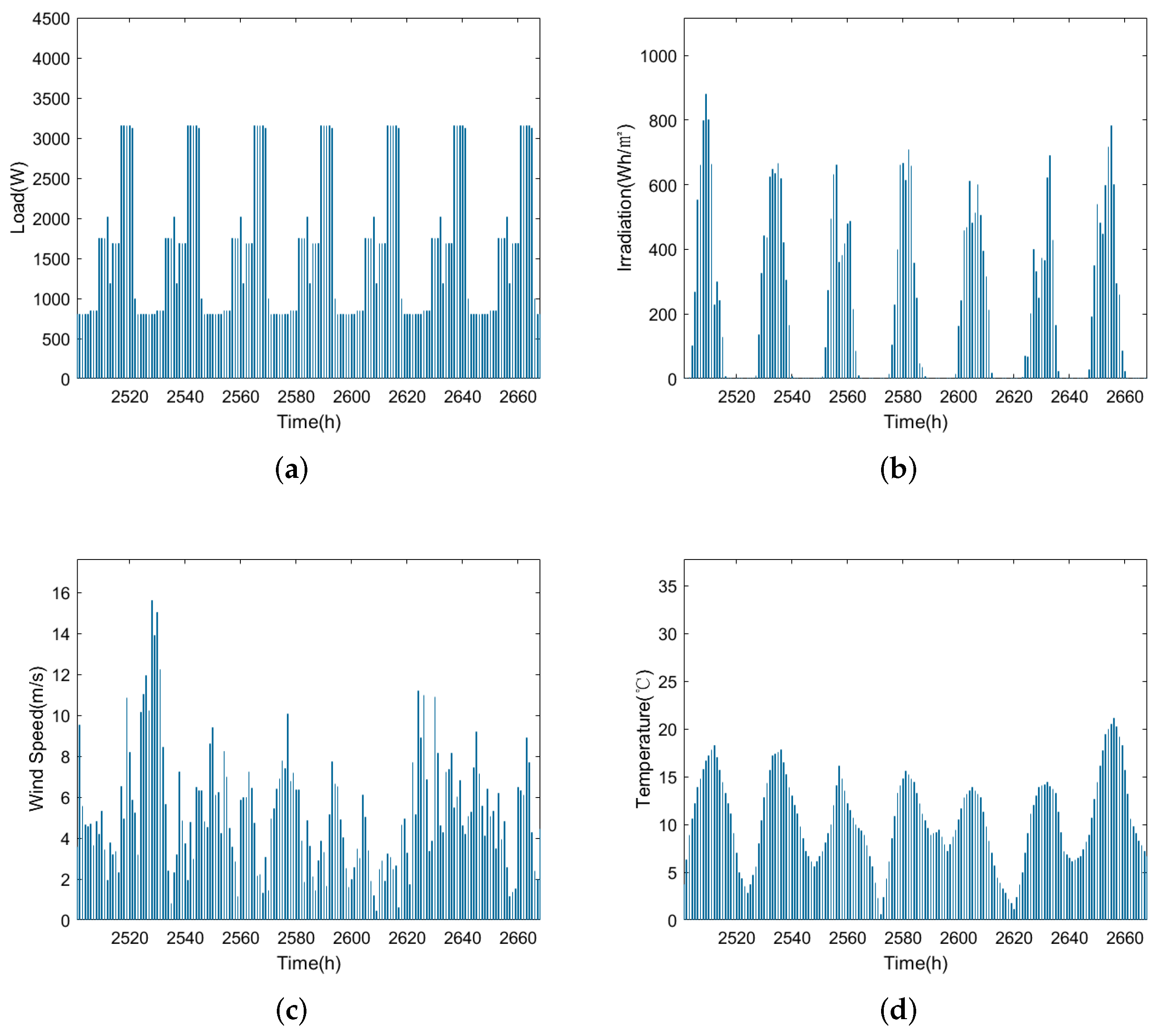
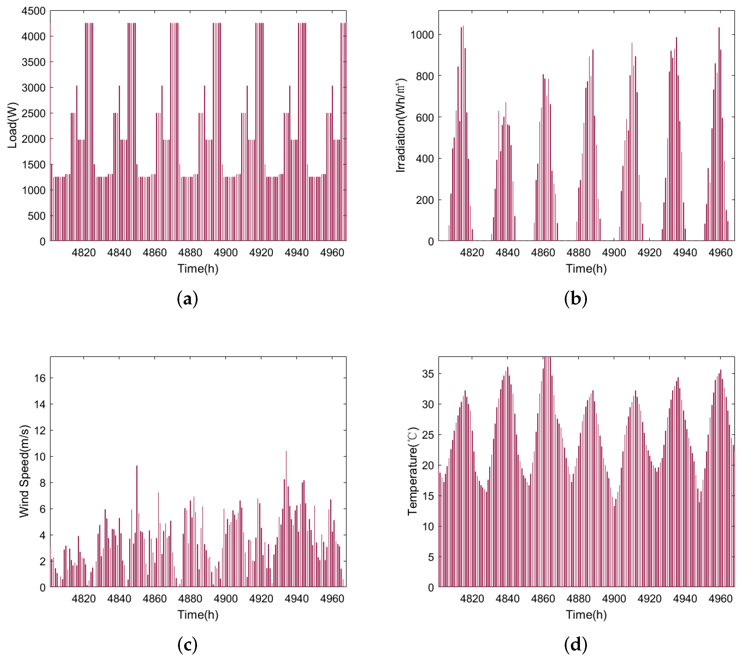
When using the PUSS model for HRES planning, the construction of a typical energy consumption scenario must first be performed, and the scenario duration and scenario data step size need to be preset. Generally speaking, the scenario duration is determined according to the planning needs and the richness of the collected data. Typical scenarios can be a typical day, a typical week, or a typical month; the step size of the scenario data should be the same as the simulation step size of the microgrid system. This study set the total scenario duration to 168 h (one week), and the scenario data step size was 1 h; the data required for the scenario were extracted from the existing data set. Because this study needed to compare the performance of multiple evolutionary algorithms in solving the PUSS problem, to quickly obtain the result data, the total number of scenarios here was temporarily set to 2; at this time, the two typical scenarios are the normal power consumption scenario and the peak power consumption scenario. See Figure 6 and Figure 7 for the specific data distribution of a typical week of normal power consumption and a typical week of peak power consumption used in the experiment.

Figure 6.
Typical week of normal power consumption. (a) Load. (b) Solar irradiation. (c) Temperature. (d) Wind speed.
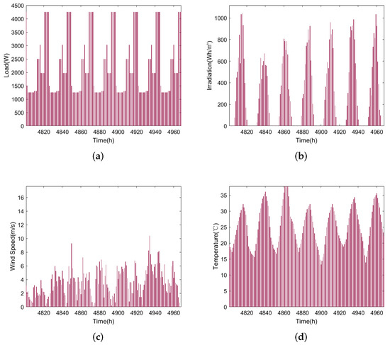
Figure 7.
Typical week of peak power consumption. (a) Load. (b) Solar irradiation. (c) Temperature. (d) Wind speed.
Among them, the typical week of peak power consumption is taken from the period when the weekly average load reaches its peak within one year; the average load of the selected typical week is about equal to the average load of the whole year. Comparing Figure 6 and Figure 7, it can be seen that the power demand, temperature, and daily solar irradiation during the typical week of peak power consumption are significantly higher than those of the typical week of normal power consumption; the daily wind speed data of the typical week of peak power consumption are lower than those of the typical week normal power consumption. For typical weekly peak power usage scenarios, higher power demand and lower wind energy resources bring greater pressure on the power supply. Although stronger solar radiation increases the amount of photovoltaic power generation, and to a certain extent alleviates the pressure of the microgrid power supply, it was not enough to offset the pressure on the microgrid power supply caused by the sharply increasing power demand in summer.
Comparing the year-round load and environmental data in Figure 5, the two types of typical weeks constructed can reflect the HRES operating conditions at ordinary times and during peak power consumption. Taking into account the environmental conditions and load data, the power supply pressure during the typical week of peak power consumption is significantly greater than the typical week of normal power consumption. Therefore, the typical week of normal power consumption was set to and the typical week of peak power consumption was set to . At this time, .
5.3. Parameter Settings
The parameters used in subsequent experiments are set here:
(1) Algorithm running times: the maximum generation number of evolution was ;
(2) Population and individuals: the population size was set to . The dimension of the decision variable for each individual in the population was , and the number of scenarios considered was . The individual coding form is:
The above variables represent the number of photovoltaic panels, wind turbines, batteries, and diesel generators, the height of the wind turbine tower, the tilt angle of the photovoltaic panels, and the occurrence probability of a typical week.
(3) The goals of the optimization are:
(4) Model constraints: For the amount of each microgrid component (///), the height of wind turbine tower , and the inclination of the photovoltaic panel , the relevant constraints of the model in [20] were adopted; for the scenario probability , needs to be met in the optimization. For other parameters of the HRES, refer to [20].
(5) Simulated binary crossover (SBX) and polynomial mutation (PM) were used as the genetic operators. Given parents and , the offspring and can be obtained by SBX as:
where is calculated according to by:
PM uses a polynomial probability distribution to make the current value of a continuous variable change to a neighboring value [28]. The crossover probability , mutation probability , and distribution index settings are shown in Table 1.

Table 1.
Settings of the algorithm parameters.
All solutions were performed based on the PlatEMO [29] platform, a well-known evolutionary multi-objective optimization platform in MATLAB. The algorithms uses the same processor for single-core single-thread calculations.
5.4. Optimization Results and Performance Evaluation
Solutions similar to that of the PUSS model can be obtained based on multiple times of solving using any scenario-based multi-objective sizing method; in the multiple times of solving, different preset combinations of scenario probabilities are used, and the final solution sets are merged, while dominated solutions are eliminated.
Therefore, in this section, based on the model and input data described in Section 2, a scenario-based dual-objective HRES optimization method using preset scenario probability combinations was selected. NSGA-II was used to perform multiple iterations and eliminate the dominated solution in the final merged solution set. It was compared with the PF obtained by the PUSS model to evaluate the performance of the PUSS model. Both methods use the same optimization goals and parameter settings.
In order to make the results of the two methods have better comparability and credibility, when the scenario-based dual-objective HRES optimization method was used to solve, the occurrence probability of the scenario was increased or decreased by 2% for each solution. To obtain the final solution set, a total of 51 times of solving was performed; when using the PUSS model to solve, the possible value of the scenario probability was also discretized in units of 2%.
As a comparison method, the scenario-based dual-objective HRES optimization method uses NSGA-II to solve the problem after presetting the scenario probability. The obtained PF quality and the solving speed are both current advanced levels [30]; when comparing the results of the PUSS model based on NSGA-II, the solution performance can be better reflected.
5.4.1. Comparison of Time Consumption
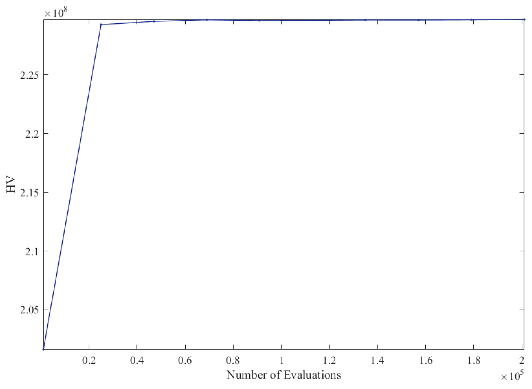
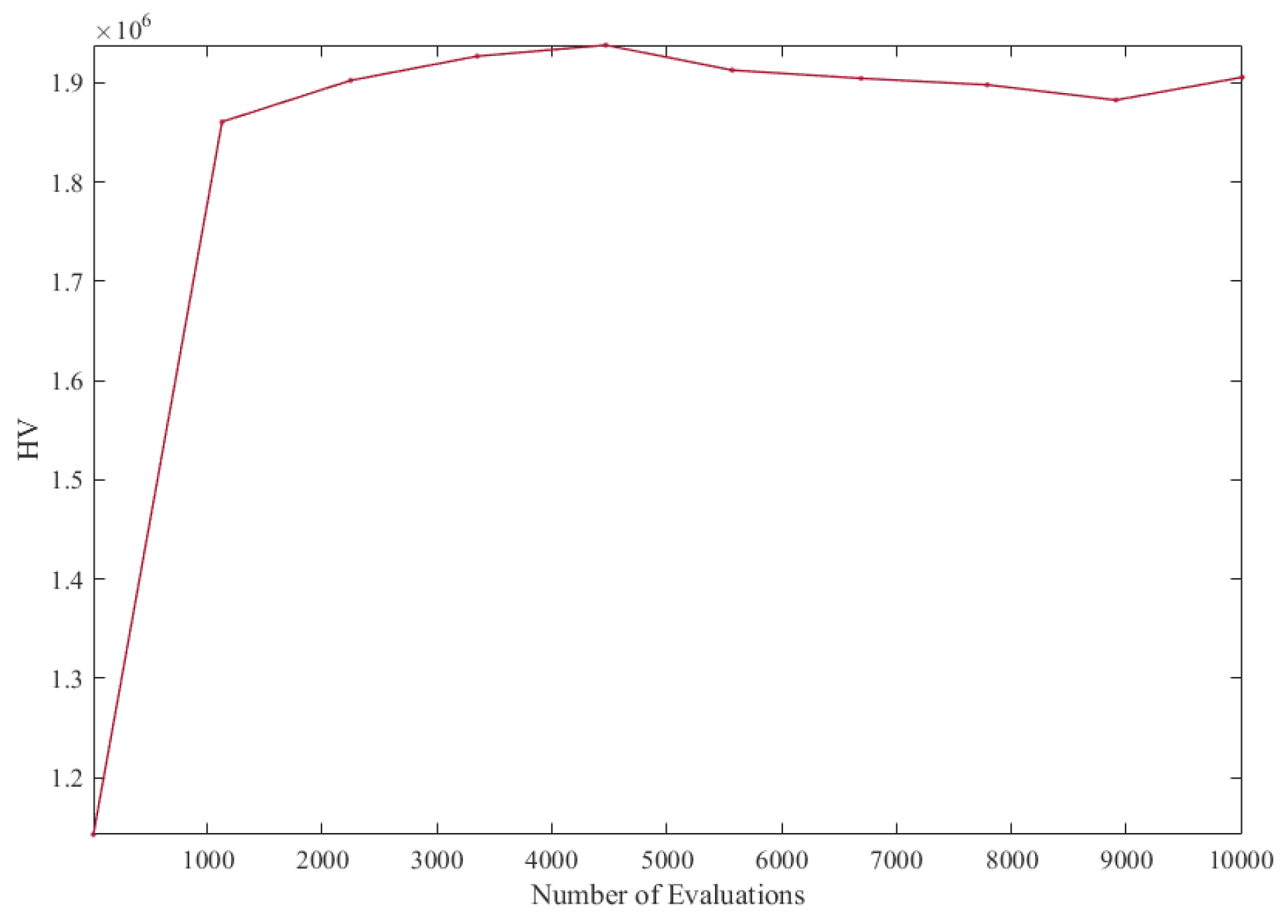
When using NSGA-II to solve the PUSS model, the population number was set to 1020 and the number of iterations was set to 200. The HV curve during the solution is shown in Figure 8; the solution took 9683.0 s and only needs to be solved once. When using NSGA-II to solve the scenario-based dual-objective HRES optimization, we set the number of population to 10 and the number of iterations to 1000. The HV curve in a single solution is shown in Figure 9; 51 iterations were needed to obtain the required solution set. In Figure 8 and Figure 9, the horizontal axis represents the times of evaluations and the ordinate is the HV value. For Figure 8, the population evolves every 1020 times of evaluation; for Figure 9, the population evolves every 10 times of evaluation.
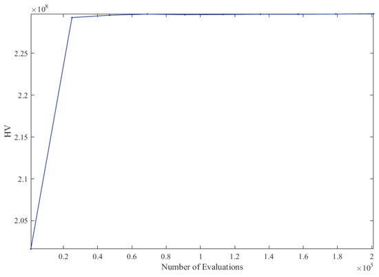
Figure 8.
HV curve of the PUSS model.
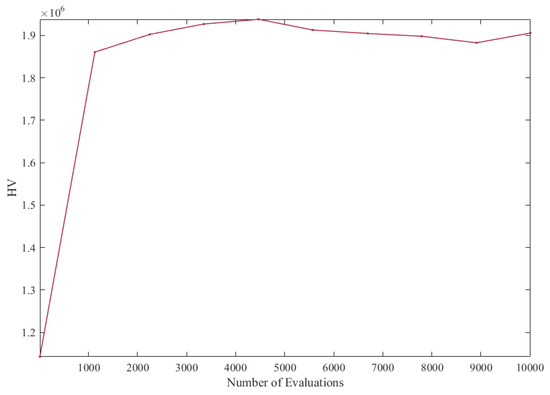
Figure 9.
HV curve of dual-objective HRES optimization.
It can be seen that using the PUSS model to perform the optimization, its solution set converged in the 70th generation (after 71,400 times of evaluations); when performing dual-objective HRES optimization, because the required population is small, the HV indicator fluctuates to a certain extent; the solution set converged in the 500th generation (after 5000 times of evaluation). The statistics are shown in Table 2.
Table 2.
Time cost data of methods.
Taking the time from the beginning of the calculation to the convergence of the solution as the time consumption of the solving method, then:
Among them, is the number of times to obtain the required PF, is the time required for a single solution, is the number of iterations required for convergence, and is the total number of iterations. As shown in Table 2, the time cost of obtaining the PF by the PUSS model was 3389.05 s; the time cost of obtaining the required solution set by the two-objective HRES optimization solution was 10,254.315 s. It can be seen that the PUSS model has significant advantages in solving time.
If the results of multiple solving using the dual-objective HRES optimization method are directly merged, the solutions in the obtained solution set may dominate each other. Therefore, in addition to the time consumed by multiple iterations, additional non-dominated sorting operations need to be performed on the solution to eliminate dominated solutions. The calculation time (6.690769 s) here should also be included in the algorithm time cost. Hence, the time consumption to obtain the Pareto front by using the dual-objective HRES optimization method multiple times was 10,261.005769 s. Furthermore, removing the dominated solution reduces the number of solutions in the solution set. Therefore, if the two-objective HRES optimization method is used to obtain the same number of solutions as the PUSS model, the actual time consumption will be slightly longer than 10,261.005769 s.
In summary, using the NSGA-II-based PUSS model for optimization, the calculation time of PF was 3389.05 s; using the dual-target HRES optimization method to obtain a solution set of the same quality required more than 10,261.005769 s. In comparison, using the PUSS model for optimization can save at least 66.97% of the time compared with the two-objective HRES optimization method; the PUSS model has a great advantage in the calculation time.
5.4.2. Performance Comparison of Solutions
Firstly, the PUSS method based on NSGA-II was used to optimize the microgrid system. To ensure the coverage of the final solution set, the number of populations was set to 1020. According to the analysis of the convergence of the previous experiments, the number of iterations was set to 125. Then, the solution set obtained by merging the solutions of 51 times of iterations using the scenario-based dual-objective HRES optimization method (based on NSGA-II) was used as a comparison; the scenario probability in the solving process started from 0% and gradually changed to 100% in 2% increments.
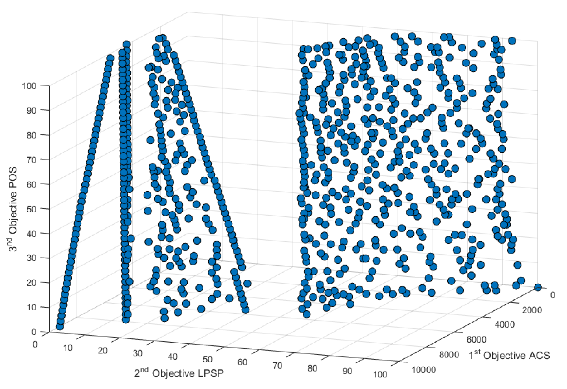
Three-dimensional PF including 1020 solutions was obtained by using the PUSS model to perform 125 iterations. After combining the 51 two-dimensional PFs obtained by solving the dual-objective HRES optimization multiple times, a solution set (also including 1020 elements), which contains mutually dominating solutions, was obtained. After ruling out the dominated solution, a three-dimensional PF with 851 solutions was obtained. The final comparison of the two PFs is shown in Figure 10 and Figure 11.
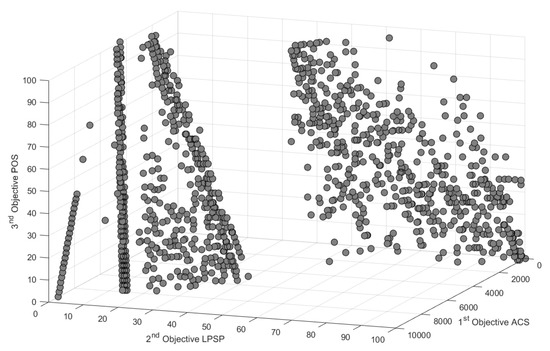
Figure 10.
PF obtained by the PUSS model.

Figure 11.
The PF obtained after 51 times of algorithm running.
For the PF shown in Figure 11, because there are many related results about using NSGA-II to solve the scenario-based dual-objective HRES optimization problem [23,24], this method is relatively mature. Therefore, it can be considered that this front can basically represent the real front.
Comparing Figure 10 and Figure 11, it can be seen that the PF obtained by the PUSS model can reflect the basic distribution of real frontiers. Due to the limitation of NSGA-II’s performance, the solution in some areas is relatively sparse; the algorithm still needs to be improved on this point. Figure 12 compares the distribution of the two fronts projected onto the X-Y(ACS-LPSP) plane, X-Z(ACS-POS) plane, and Y-Z (LPSP-POS) planes; grey is the projection of the PF obtained by the PUSS model, and blue is the projection of the PF obtained after the merged solution results are processed. It can be seen that the distribution of the PF solution obtained by the PUSS model on the X-Y plane is close to the true front; the distribution of the solutions on the X-Z and Y-Z planes forms a situation of clustering along a certain centerline, and the solution is very sparse in the area far from the centerline. In later work, the PUSS model can be further adjusted and improved to address this problem.
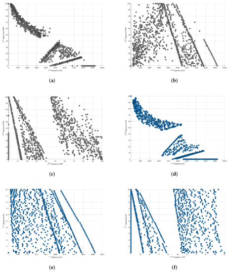
Figure 12.
Contrast of 2D PF projections. (a) PF obtained by the PUSS method projected onto the X-Y(ACS-LPSP) plane. (b) PF obtained by the PUSS projected onto the X-Z(ACS-POS) plane. (c) PF obtained by the PUSS method projected onto the and Y-Z (LPSP-POS) planes. (d) PF obtained by the compared method projected onto the X-Y(ACS-LPSP) plane. (e) PF obtained by the compared projected onto the X-Z(ACS-POS) plane. (f) PF obtained by the compared method projected onto the and Y-Z (LPSP-POS) planes.
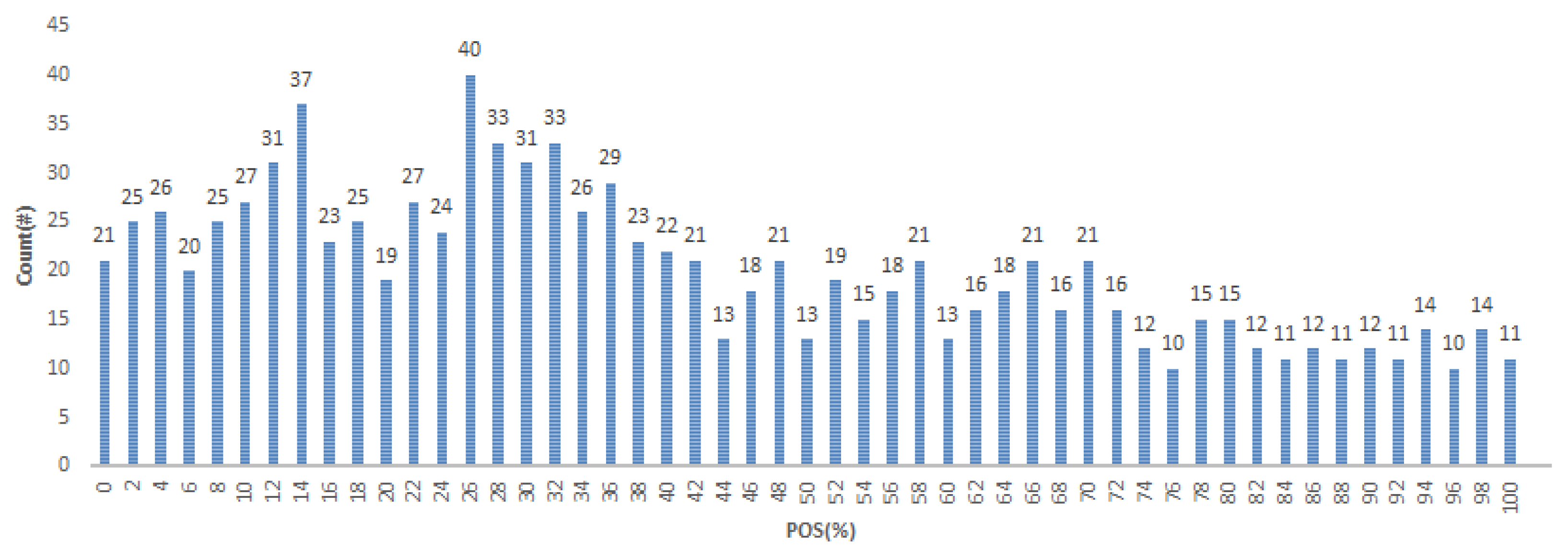
Figure 13 gives the statistics of the distribution of the number of solutions of the Pareto front obtained by the PUSS model under different scenario probabilities (). It can be seen from the figure that the 51 possible values of are all covered. In the PF with a total of 1020 solutions, there should be an average of 20 solutions for each value of . In the actual solution results, there are at least 10 solutions and a maximum of 40 solutions for each value of . When the value of is small, the corresponding number of solutions is relatively large, and vice versa; although the number of solutions changes according to this trend, there is a certain fluctuation in the specific number.
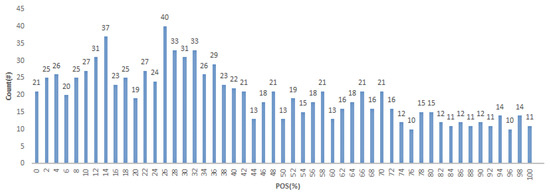
Figure 13.
Distribution of solutions obtained by the PUSS model under different scenario probabilities.
In summary, there is no need to obtain a PF including a very large amount of solutions. Without a very large number of solutions in the PF, the results of the PUSS model can cover all possible values of . When the expectation of the number of solutions corresponding to each being 20, at least 10 solutions can be guaranteed for all possible values. The solution results of the PUSS model can reflect the overall situation of the configuration scheme under different scenario probability combinations and provide sufficient alternatives under each scenario probability combination.
To compare the quality of the solutions in the two PFs, the solutions in the two PFs are labeled separately and then combined into a set for non-dominated sorting. Then, we calculate the number of remaining non-dominated solutions separately. The results are shown in Table 3. By statistics, after merging the PF into a set and excluding the dominated solution, the remaining non-dominated solutions accounted for 80.29% (PF obtained by PUSS) and 84.61% (3D PF obtained by excluding the dominated solution after merging 2D PF) of the original PF. It can be seen that the optimality of the solutions in the two PFs is basically the same.
Table 3.
Settings of algorithm parameters.
6. Conclusions
Because the traditional HRES configuration optimization considering the influence of uncertainty has a large dependence on actual data, or it cannot effectively utilize the existing data information in the application, this paper proposed a probability undetermined scenario-based sizing model (PUSS model) to solve the above problems and provide a set of configuration schemes that can cope with various maximum environmental uncertainties.
In this study, the optimization results obtained by the PUSS model (based on NSGA-II) were compared with the configuration schemes obtained by using the scenario-based dual-objective HRES optimization method (also based on NSGA-II) multiple times. This comparison showed that the solution of the PUSS model only took about 33% of the time of the other method, and the performance of the PF obtained by the two methods was basically equivalent in terms of the optimality of the solutions; the solution results of the PUSS model can cover all scenario probability combinations and provide no less than half the mathematical expectation of the number of solutions for each possible scenario probability combination.
When comparing the results of these two methods, the dominated solutions in the solution set obtained by using the dual-objective HRES optimization method multiple times were first eliminated. Based on multiple times of solving, solutions similar to that of the PUSS model can be obtained using any scenario-based multi-objective sizing method. In this solving process, different preset combinations of scenario probabilities were used, and the final solution sets need to be merged to obtain the solution set. It must be pointed out that this solution set is essentially different from the results obtained by the PUSS model. In the solution set of the PUSS model, the individuals do not dominate each other. That is, each solution is optimal in this solution set. For the results obtained by solving the traditional scenario-based method multiple times, although there must be no Pareto dominance between the solutions under a certain combination of scenario probabilities, the solutions between different scenario probability combinations may dominate each other. In other words, the result obtained by solving multiple times and merging is not a Pareto set and cannot be directly used by decision-makers.
In comparison, the solution set obtained by the PUSS model is sparse in some regions and too dense in other regions. Further research is needed to address this problem: improve NSGA-II’s adaptively or select more appropriate algorithms and perform adjustments accordingly. Though the PUSS model describes the uncertainty caused by renewable energy fluctuations in HRES planning in the form of scenarios and their occurrence probabilities, it is not required to determine the corresponding occurrence probability of each scenario before the optimization. In this way, the PUSS model solves the problem to a certain extent as the probability corresponding to a scenario is difficult to determine when using the traditional method to deal with uncertain factors; the PUSS model also avoids the problem of it being difficult to fully use the existing information to describe uncertain parameters in the form of intervals. Besides, solving the PUSS model, we can obtain the optimal set under a variety of scenario probability combinations, which can deal with multiple degrees of maximum environmental uncertainty and reflect the relationship between the microgrid optimization objective values of the configuration scheme and the maximum environmental uncertainty that the configuration scheme can withstand. In the case where the optimality of the optimization results of the two methods is equivalent, the calculation speed of the PUSS model has obvious advantages over the alternative method.
If the number of scenarios to be considered is high, the number of objectives will also be high. In this case, more Pareto solutions are needed to characterize the Pareto front, which will lead to high computational cost. Future works can investigate more efficient many-objective optimization algorithms for the cases with a large number of scenarios. Moreover, the long execution time of the algorithms mainly results from the large computational burden of the simulation process that is used to compute the objectives. Future works can investigate efficient proxy model to estimate the objectives, which can improve the efficiency of the optimization algorithms significantly.
Author Contributions
Conceptualization, R.W.; methodology, K.L. and Y.S.; validation, K.L.; investigation, K.L.; resources, Y.S.; data curation, Y.S.; writing—original draft preparation, K.L.; writing—review and editing, K.L.; visualization, K.L. All authors have read and agreed to the published version of the manuscript.
Funding
This research was funded by the Hunan Youth elite program (2018RS3081) and the key project of National University of Defense Technology (ZK18-02-09). This paper is partially supported by the National Natural Science Foundation of China (No. 72071205 and No. 61773390).
Institutional Review Board Statement
Not applicable.
Informed Consent Statement
Not applicable.
Data Availability Statement
Not applicable.
Conflicts of Interest
The authors declare no conflict of interest. The funders had no role in the design of the study; in the collection, analyses, or interpretation of the data; in the writing of the manuscript; nor in the decision to publish the results.
References
- Alsmadi, Y.M.; Abdel-hamed, A.M.; Ellissy, A.E.; El-Wakeel, A.S.; Abdelaziz, A.Y.; Utkin, V.; Uppal, A.A. Optimal configuration and energy management scheme of an isolated micro-grid using Cuckoo search optimization algorithm. J. Frankl. Inst. 2019, 356, 4191–4214. [Google Scholar] [CrossRef]
- Rubio-Maya, C.; Uche-Marcuello, J.; Martínez-Gracia, A.; Bayod-Rújula, A.A. Design optimization of a polygeneration plant fuelled by natural gas and renewable energy sources. Appl. Energy 2011, 88, 449–457. [Google Scholar] [CrossRef]
- Zhang, J.; Lei, Y.; Liu, N.; Rui, X. Capacity Configuration Optimization for Island Microgrid with Wind/Photovoltaic/Diesel/Storage and Seawater Desalination Load. Trans. China Electrotech. Soc. 2014, 29, 102–112. [Google Scholar]
- Guelpa, E.; Marincioni, L.; Capone, M.; Deputato, S.; Verda, V. Thermal load prediction in district heating systems. Energy 2019, 176, 693–703. [Google Scholar] [CrossRef]
- Fan, C.; Xiao, F.; Zhao, Y. A short-term building cooling load prediction method using deep learning algorithms. Appl. Energy 2017, 195, 222–233. [Google Scholar] [CrossRef]
- Li, K.; Wang, R.; Lei, H.; Zhang, T.; Liu, Y.; Zheng, X. Interval prediction of solar power using an Improved Bootstrap method. Sol. Energy 2018, 159, 97–112. [Google Scholar] [CrossRef]
- Mavromatidis, G.; Orehounig, K.; Carmeliet, J. Design of distributed energy systems under uncertainty: A two-stage stochastic programming approach. Appl. Energy 2018, 222, 932–950. [Google Scholar] [CrossRef]
- Bornapour, M.; Hooshmand, R.A.; Parastegari, M. An efficient scenario-based stochastic programming method for optimal scheduling of CHP-PEMFC, WT, PV and hydrogen storage units in micro grids. Renew. Energy 2019, 130, 1049–1066. [Google Scholar] [CrossRef]
- Bornapour, M.; Hooshmand, R.A.; Khodabakhshian, A.; Parastegari, M. Optimal stochastic scheduling of CHP-PEMFC, WT, PV units and hydrogen storage in reconfigurable micro grids considering reliability enhancement. Energy Convers. Manag. 2017, 150, 725–741. [Google Scholar] [CrossRef]
- Akbari, K.; Nasiri, M.M.; Jolai, F.; Ghaderi, S.F. Optimal investment and unit sizing of distributed energy systems under uncertainty: A robust optimization approach. Energy Build. 2014, 85, 275–286. [Google Scholar] [CrossRef]
- Majewski, D.E.; Lampe, M.; Voll, P.; Bardow, A. TRusT: A Two-stage Robustness Trade-off approach for the design of decentralized energy supply systems. Energy 2017, 118, 590–599. [Google Scholar] [CrossRef]
- Yokoyama, R.; Fujiwara, K.; Ohkura, M.; Wakui, T. A revised method for robust optimal design of energy supply systems based on minimax regret criterion. Energy Convers. Manag. 2014, 84, 196–208. [Google Scholar] [CrossRef] [Green Version]
- Moret, S.; Bierlaire, M.; Maréchal, F. Robust optimization for strategic energy planning. Informatica 2016, 27, 625–648. [Google Scholar] [CrossRef] [Green Version]
- Bertsimas, D.; Litvinov, E.; Sun, X.A.; Zhao, J.; Zheng, T. Adaptive robust optimization for the security constrained unit commitment problem. IEEE Trans. Power Syst. 2012, 28, 52–63. [Google Scholar] [CrossRef]
- Dong, C.; Huang, G.H.; Cai, Y.P.; Liu, Y. Robust planning of energy management systems with environmental and constraint-conservative considerations under multiple uncertainties. Energy Convers. Manag. 2013, 65, 471–486. [Google Scholar] [CrossRef]
- Liu, Y.; Lei, H.; Zhang, D.; Wu, Z. Robust optimization for relief logistics planning under uncertainties in demand and transportation time. Appl. Math. Model. 2018, 55, 262–280. [Google Scholar] [CrossRef]
- Gulpinar, N.; Pachamanova, D.; Çanakoğlu, E. Robust strategies for facility location under uncertainty. Eur. J. Oper. Res. 2013, 225, 21–35. [Google Scholar] [CrossRef]
- Kouvelis, P.; Yu, G. Robust Discrete Optimization and Its Applications; Springer Science & Business Media: Berlin/Heidelberg, Germany, 2013; Volume 14. [Google Scholar]
- Halpern, J.Y.; Leung, S. Weighted sets of probabilities and minimax weighted expected regret: A new approach for representing uncertainty and making decisions. Theory Decis. 2015, 79, 415–450. [Google Scholar] [CrossRef]
- Song, Y.; Liu, Y.; Wang, R.; Ming, M. Multi-Objective Configuration Optimization for Isolated Microgrid with Shiftable Loads and Mobile Energy Storage. IEEE Access 2019, 7, 95248–95263. [Google Scholar] [CrossRef]
- Deb, K.; Pratap, A.; Agarwal, S.; Meyarivan, T. A fast and elitist multiobjective genetic algorithm: NSGA-II. IEEE Trans. Evol. Comput. 2002, 6, 182–197. [Google Scholar] [CrossRef] [Green Version]
- Zitzler, E.; Laumanns, M.; Thiele, L. SPEA2: Improving the Strength Pareto Evolutionary Algorithm; TIK-Report 103; ETH Zurich: Zurich, Switzerland, 2001. [Google Scholar]
- Zitzler, E.; Künzli, S. Indicator-based selection in multiobjective search. In International Conference on Parallel Problem Solving from Nature; Springer: Berlin/Heidelberg, Germany, 2004; pp. 832–842. [Google Scholar]
- Zhang, Q.; Li, H. MOEA/D: A multiobjective evolutionary algorithm based on decomposition. IEEE Trans. Evol. Comput. 2007, 11, 712–731. [Google Scholar] [CrossRef]
- Cheng, R.; Jin, Y.; Olhofer, M.; Sendhoff, B. A reference vector guided evolutionary algorithm for many-objective optimization. IEEE Trans. Evol. Comput. 2016, 20, 773–791. [Google Scholar] [CrossRef] [Green Version]
- Buayai, K.; Ongsakul, W.; Mithulananthan, N. Multi-objective micro-grid planning by NSGA-II in primary distribution system. Eur. Trans. Electr. Power 2012, 22, 170–187. [Google Scholar] [CrossRef]
- Lu, X.Y.; Huang, Y.Q.; Liu, N.; Zhang, J.H.; Huang, L.Z. A Study of Optimal Capacity Configuration with multi-Objective for Islanded Micro-grid. Appl. Mech. Mater. Trans. Tech. Publ. 2014, 521, 464–468. [Google Scholar] [CrossRef]
- Deb, K.; Agrawal, R.B. Simulated binary crossover for continuous search space. Complex Syst. 1995, 9, 115–148. [Google Scholar]
- Tian, Y.; Cheng, R.; Zhang, X.; Jin, Y. PlatEMO: A MATLAB platform for evolutionary multi-objective optimization [educational forum]. IEEE Comput. Intell. Mag. 2017, 12, 73–87. [Google Scholar] [CrossRef] [Green Version]
- Zhichao, S. Research on Hybrid Renewable Energy System Planning Based on Multi-Objective Evolutionary Algorithm. Ph.D. Thesis, National University of Defense Technology, Changsha, China, 2016. [Google Scholar]


Publisher’s Note: MDPI stays neutral with regard to jurisdictional claims in published maps and institutional affiliations. |
© 2022 by the authors. Licensee MDPI, Basel, Switzerland. This article is an open access article distributed under the terms and conditions of the Creative Commons Attribution (CC BY) license (https://creativecommons.org/licenses/by/4.0/).