Adaptive Differential Evolution Algorithm Based on Fitness Landscape Characteristic

Abstract

Differential evolution (DE) is a simple, effective, and robust algorithm, which has demonstrated excellent performance in dealing with global optimization problems. However, different search strategies are designed for different fitness landscape conditions to find the optimal solution, and there is not a single strategy that can be suitable for all fitness landscapes. As a result, developing a strategy to adaptively steer population evolution based on fitness landscape is critical. Motivated by this fact, in this paper, a novel adaptive DE based on fitness landscape (FL-ADE) is proposed, which utilizes the local fitness landscape characteristics in each generation population to (1) adjust the population size adaptively; (2) generate DE/current-to-pcbest mutation strategy. The adaptive mechanism is based on local fitness landscape characteristics of the population and enables to decrease or increase the population size during the search. Due to the adaptive adjustment of population size for different fitness landscapes and evolutionary processes, computational resources can be rationally assigned at different evolutionary stages to satisfy diverse requirements of different fitness landscapes. Besides, the DE/current-to-pcbest mutation strategy, which randomly chooses one of the top p% individuals from the archive cbest of local optimal individuals to be the pcbest, is also an adaptive strategy based on fitness landscape characteristic. Using the individuals that are approximated as local optimums increases the algorithm’s ability to explore complex multimodal functions and avoids stagnation due to the use of individuals with good fitness values. Experiments are conducted on CEC2014 benchmark test suit to demonstrate the performance of the proposed FL-ADE algorithm, and the results show that the proposed FL-ADE algorithm performs better than the other seven highly performing state-of-art DE variants, even the winner of the CEC2014 and CEC2017. In addition, the effectiveness of the adaptive population mechanism and DE/current-to-pcbest mutation strategy based on landscape fitness proposed in this paper are respectively verified.

1. Introduction

Optimization problems are universal in nature, because most problems in real life can be expressed by optimization models, involving multiple standards and goals. Researchers are concentrating their efforts on broad algorithms that may be used for a variety of issues. The development of such general purpose algorithms, which can be categorized as meta-heuristics, has accelerated over the last few decades. Differential evolution (DE) is a basic but powerful algorithm that belongs to the evolutionary algorithms category (EA). DE is a population-based algorithm of metaheuristics, conceptualized by Storn and Price [1]. DE has become a popular choice among researchers for tackling optimization issues in a variety of disciplines over the last two decades [2], such as vehicle routing problems [3], power engineering problems [4], wireless sensors [5], the medical field [6], and chemical engineering [7].

Similar to other evolutionary algorithms (EAs), such as genetic algorithm (GA) [8], memetic algorithm (MA) [9], and estimation of distribution algorithm (EDA) [10], DE also contains three evolutionary operators, namely, mutation, crossover, and selection. The most significant phase in DE is mutation, which is also a crucial step in the production of new individuals by adding a weighted difference vector between two individuals in a population to the third. The essence of mutation is a search behavior, which can prevent premature convergence by increasing population diversity. Over the past decades, many mutation strategies, such as DE/rand-to-best/1, DE/lbest/1 [11], DE/current-to-pbest/1 [12], and ranking-based mutation [13], have been developed for DE. Shen and He [14] presented a mixed mutation strategy. The algorithm collects local fitness landscape characteristics based on each individual’s fitness changes over the distance between each person and the best individual and then uses the Gaussian Cauchy mutation to choose variants of the probability distribution of an optimal mixing strategy. Generally, different strategies display distinct characteristics and are suitable for different fitness landscape characteristics of the evolutionary process.

DE is made up of three main parameters: (1) population size N, which specifies the number of selection operations performed in each generation, (2) scaling factor F, which limits the differential mutation operation, and (3) crossover rate CR, which specifies how many parameters in the target vector altered during the crossover operation [15]. Three parameters suggested respectively by DE inventors Storn and Price [16] are: (1) N ∈ [5D,10D], D is the dimension of the problem, and N = 100 is recommended as the initial value; (2) F ∈ [0.4,1], and F = 0.5 is sufficient for obtaining an optimal solution; (3) for unimodal separable functions, CR ∈ [0, 1] and CR = 0.1 are appropriate initial values, while CR = 0.9 is a good initial value for multimodal and nonseparable functions. Besides, other corresponding DE control parameters are also suggested in references [17,18]. Compared to fixed control parameter values, the adaptive control parameter mechanism performs better. Different adaptive or self-adaptive mechanisms (such as FADE [19], ADE [20], jDE [21], JADE [12], SHADE [22], SinDE [23]) are introduced to dynamically update control parameters F and CR without a user’s prior knowledge of the relationship between parameter settings and the features of an optimization problem. Apparently, good adaptive parameter design can improve the convergence performance of the algorithm. Since 2013, Tanabe and Fukunaga’s SHADE [22] has become a common denominator for the top DE variations [24]. To assist the selection of future control parameter values, this method leveraged a historical recollection of previous control parameter choices.

Although the number of parameters of the differential evolution is small, different hyperparameters and differential evolution variants, such as different mutation operators and F and CR parameters, may introduce structural biases. Structural bias is a form of bias in which artifacts in an algorithm lead to a preference for specific regions in the search space, independent of the objective function [25,26]. What’s more, previous work [26,27] on structural bias has pointed out that the strategy for dealing with infeasible solutions can have a huge impact on the presence and strength of structural bias. The choice of the strategy for dealing with infeasible solutions is of high importance, in particular for highly multidimensional problems, as it is more likely to generate infeasible solutions [28]. After analyzing the structural bias of a large number of DE algorithms, Diederick et al. [25] concluded that it is safest to use the dismiss strategy because this strategy for dealing with infeasible solutions shows almost no structural bias, which is consistent with the intersection of the operator being independent of population size. The proposed FL-ADE algorithm inherits the dismiss strategy for dealing with infeasible solutions of LSHADE [29].

However, most of the proposed adaptive DE variants modify the values of F and CR, change the DE strategy, but use a fixed population size. Only a few papers deal with the adaptation of the population size even though the population size is also a crucial parameter of DE, which affects the search efficiency [30]. It can be said that the most popular method of population size control is applied in L-SHADE variant [29]. It is a simple and effective deterministic population size that linearly decreases with the number of evaluations proposed by Tanabe and Fukunaga. The efficiency of the L-SHADE algorithm was confirmed by its first position in the competition of CEC2014 [31]. The same “L” approach was also used in another DE variant typically derived from the L-SHADE algorithm. However, there are few studies on the size of adaptive population. Poláková et al. [32] proposed an adaptive mechanism of population size according to current population diversity. Zhan et al. proposed adaptive distributed differential evolution ADDE [33], which describes an adaptive population parameter setting based on best solution improvement (BSI). This article proposes a new mechanism for population size adaptation based on the fitness landscape.

In recent years, there have been some DE variants based on the fitness landscape. Based on fitness landscape research, Huang et al. devised a self-feedback strategy differential evolution (SFSDE) method [34]. By extracting the features of the local fitness landscape, Li et al. [35] proposed a new self-feedback DE algorithm (SFDE) that selected the optimal mutation strategy and calculated the probability distributions of single-modality and multimodality. Tan et al. recently proposed a DE with an adaptive mutation operator based on fitness landscape (FLDE) [36], which analyzed the fitness landscape features of 45 benchmark training functions before training the relationship between three mutation strategies and fitness landscape features offline using random forest (RF). Finally, throughout the evolutionary process, the trained RF is used to anticipate which mutation technique should be employed to perform mutation operator for each problem. The suggested FLDE algorithm is very competitive with the other five well-known DE algorithms, according to the experimental results. Although there are some DE variants based on the fitness landscape, they all focus on selecting mutation strategies.

The fitness landscape can be used to assess the complexity of an optimization issue in general. However, even though fitness landscape can be used to define the optimization problem and study the evolutionary process, it is rarely used to create algorithms [36]. An adaptable DE based on fitness landscape features (FL-ADE) is proposed in this work. The following are the paper’s major contributions:

• A novel adaptive mechanism of the population size based on the fitness landscape enables the reduction of the population size when exploration is needed and the increase in the population size when exploitation is needed. Most importantly, all these changes in population size are adaptive by extracting the local fitness landscape characteristics and do not require the introduction of any additional parameters.
• A new mutation strategy: DE/current-to-pcbest, which utilizes the individuals of the approximate local optimum, increases the capability of exploration in multimodal fitness landscape and avoids falling into local optimal due to the use of good function values.

As we can see, FL-ADE takes advantage of the approximate local optimal individuals for the mutation strategy DE/current-to-pcbest to search for different potential regions according to the fitness landscape of different functions. In addition, the fitness landscape characteristics of each generation are calculated, so as to adjust the population size adaptively. The novelty of FL-ADE is that there is no need to use different strategies and set the corresponding population size in advance according to the characteristics of the function. Regardless of any kind of problem, unimodal, multimodal, composite, and hybrid functions, FL-ADE can adaptively focus on different search strategies. On unimodal functions, FL-ADE makes more use of good fitness values, while maintaining a relatively small population size and quickly converging to the global optimum. In contrast, in the face of multimodal functions and complex functions, FL-ADE will use more potential approximate local optimal values, while maintaining a large population size in the early stage to maintain the diversity of the population. In the later stage or when it almost converges to the optimal region, it reduces the population size to increase the iteration speed and quickly converge. The experimental results on CEC2014 benchmark test suite compared with the seven powerful state-of-art DE, even the winner of the CEC2014 and CEC2017.

The rest of the paper is laid out as follows: The classic DE and LSHADE’s adaptive parameter process, as well as fitness landscape characteristics, are briefly described in Section 2. The planned FL-ADE is then shown in Section 3. Section 4 contains the experimental results as well as a discussion. The Section 5 gives the conclusions and makes a prospect for the future research.

2. Material Method

In this section, the classic DE is introduced. In addition, the adaptive parameter mechanism and linear population size reduction mechanism of LSHADE is described. Finally, the fitness landscape characteristics are introduced.

2.1. Differential Evolution

The standard DE algorithm consists of four parts.

(1)

Initialization: The initial population is randomly generated within a given boundary domain as:

$$x_{i,j}^G=x_j^{min}+rand\left(0,1\right)\times \left(x_j^{max}-x_j^{min}\right)$$

(1)

where $i=1,2,\dots ,N$ and $j=1,2,\dots ,D$. Herein, N represents the population size, D is the problem dimension, rand(0,1) is a set of random numbers uniformly distributed in the interval of (0, 1), and $x_j^{max}$ and $x_j^{min}$ denote the upper and lower boundaries of the jth dimension, respectively.

(2)

Mutation operator: At each generation, a mutation vector $v_i$ is generated based on the difference between two individuals. Here, we list some classic mutation strategies as follows:

DE/rand/1:

$$v_i=x_{r1}+F\times \left(x_{r2}-x_{r3}\right)$$

(2)

DE/best/1:

$$v_i=x_{best}+F\times \left(x_{r1}-x_{r2}\right)$$

(3)

DE/current-to-best/1:

$$v_i=x_i+F\times \left(x_{best}-x_i\right)+F\times \left(x_{r1}-x_{r2}\right)$$

(4)

DE/current-to-best/1:

$$v_i=x_i+F\times \left(x_{best}^p-x_i\right)+F\times \left(x_{r1}-{\tilde{x}}_{r2}\right)$$

(5)

where $v_i=[v_{i,1},v_{i,2},\dots v_{i,D}]$, $r1,r2,r3\in [1,2,\dots ,N]$, $i\ne r1\ne r2\ne r3$ and F is the scaling factor. $x_{best}$ is the best individual, which has the best fitness value in the current population. $x_{best}^p$ is randomly chosen from the top 100 × N × p% individuals in the current population with p ⊂ (0,1). ${\tilde{x}}_{r2}$ is randomly chosen from the union of P and A, where P is the set of the current population and A is the set of archived inferior solutions [12].

(3)

Crossover Operator: Trial vector u_i is formed by the individuals x_i and v_i, where $u_i=[u_{i,1},u_{i,2},\dots ,u_{i,D}]$. In general, there are two classic crossover operators, namely, binomial crossover and exponential crossover. In this paper, the binomial cross is adopted.

In the binomial crossover, each dimension of u_i is separately determined to come from v_i and x_i by the parameter of crossover rate CR as:

$$u_{i,j}=\left\{\begin{array}{l}{v}_{i,j}, if rand\left(0,1\right) \le C{R}_i or j=j_{rand}\\ x_{i,j}, otherwise\end{array}\right.$$

(6)

where rand(0,1) is a random number between 0 and 1, while the jrand is a random index in [1, 2, ..., D] to ensure that at least one dimension of u_i comes from v_i.

(4)

Selection Operator: The selection operation procedure is to compare the objective values of target vector x_i and trial vector u_i for the minimization problem by using Equation (7), which means that the better one will be selected for the next generation.

$$x_i^{G+1}=\left\{\begin{array}{l}{u}_i^G, if f\left(u_i^G\right)<f\left(x_i^G\right)\\ x_i^G, otherwise\end{array}\right.$$

(7)

The DE repeats the above mutation, crossover, and selection operators until it satisfies the terminal conditions.

2.2. LSHADE

The SHADE [22] algorithm is a better variant of JADE because it employs a different parameter adaptation mechanism based on success history-based adaptation, which is a useful technique for parameter adaptation based on the historical memory of successful parameter sets throughout iteration. Success history-based parameter adaptation employs a historical memory M_CR, M_F, which retains a set of CR and F values that have worked successfully in the past and produces new CR and F pairs by selecting them at random. By introducing a linear population size reduction method as well as changes to parameters such as H, |A|, and CR, where H is the number of entries into the successfully historical memory pool and |A| is the size of external archive, the LSHADE [29] algorithm enhanced the overall optimization performance of SHADE. All of these adjustments helped LSHADE win the first place in the CEC2014 competition. Recently proposed strong DE variants, such as iLSHADE [37], jSO [38], PaDE [39], and LSHADE_cnEpSin [40], are all variants of LSHADE. LSHADE mainly includes the adaptive parameter mechanism based on success history, as well as a linear population size reduction mechanism (LPSR). This paper also uses LSHADE’s adaptive parameter mechanism based on success history, and the proposed adaptive population size mechanism FL-APS is also combined with LPSR, so this chapter will introduce LSHADE. For the linear population size reduction mechanism, Equation (8) depicts the detailed change of N during evolution for the population size reduction mechanism:

$$N_{G+1}^{Linear}=round\left[\left(\frac{N^{min}-N^{init}}{FESmax}\right)\times FES\right]+N^{init}$$

(8)

where the N^init is the initial population size, N^min is the minimum population size, FES_max denotes the maximum number of function evaluations, FES denotes the current number of function evaluations, and round[∙] means “round to the nearest integer”.

This paper uses the parameter adaptation mechanism of LSHADE. In each generation, in Equation (7), CR and F values that succeed in generating a trial vector $u_i^G$ which is better than the parent individual $x_i^G$ are recorded as S_CR, S_F, and at the end of the generation, the memory of M_CR, M_F is updated using Algorithm 1. The position in memory to update is determined by the index k(1 ≤ k ≤ H). The k-th element in the memory is updated in generation G. k is set to 1 at the start of the search and is incremented whenever a new element is added to the history. If k > H, k is set to 1. S_CR and S_F denote the success sets of control parameters F and CR, and “success” means that a certain individual employing these control parameters produces an offspring with better fitness value. The memory is not updated when all individuals in generation G fail to develop a trial vector that is better than the parent, i.e., S_CR = S_F = ∅.

Algorithm 1: Memory update algorithm in LSHADE

1 Input: the success set $S_{CR}$ and $S_F$ 2 Output: the historical memory $M_{CR}$ and $M_F$ 3 If $S_{CR}\ne \varnothing$ and $S_F\ne \varnothing$ then 4  If $M_{CR,k,G}=\perp$ or $\max \left(S_{CR}\right)=0$ then 5   $M_{CR,k,G+1}=\perp$; 6 Else 7   $M_{CR,k,G+1}=mea{n}_{WL}\left(S_{CR}\right)$; 8  End If 9 $M_{F,k,G+1}=mea{n}_{WL}\left(S_F\right)$; 10  $k++$; 11  If $k>H$, then $k=1$; End If 12 Else 13 $M_{CR,k,G+1}=M_{CR,k,G}$; 14 $M_{F,k,G+1}=M_{F,k,G}$; 15. End If

As M_CR is updated, if $M_{CR,k,G=\perp }$ (where ⊥ denotes a special, “terminal value”) or max(S_CR) = 0 (i.e., all elements of S_CR are 0), $M_{CR,k,G+1}$ is set to ⊥. The weighted Lehmer mean mean_WL (S) is computed using the formula below, and as with [41], the amount of fitness improvement $\Delta f_k$ is used in order to influence the parameter adaptation (S refers to either S_CR or S_F).

$$\left\{\begin{array}{l}mea{n}_{WL}\left(S\right)=\frac{{{\displaystyle \sum }}_{k=1}^{\left|S\right|}{w}_k\times S_k^2}{{{\displaystyle \sum }}_{k=1}^{\left|S\right|}{w}_k\times S_k}\\ w_k=\frac{\Delta f_k}{{{\displaystyle \sum }}_{l=1}^{\left|S_{CR}\right|}\Delta f_l}\\ \Delta f_k=\left|f\left(u_k^G\right)-f\left(x_k^G\right)\right|\end{array}\right.$$

(9)

2.3. Fitness Landscape Characteristics

2.3.1. Definition of Fitness Landscape

Fitness landscape, as defined by Wright, is a static model of the problem that has been shown to be effective for examining evolution methods [42]. Consider a continuous function f(x), where $x\in R^n$, where n is the dimension of problem. A fitness landscape in a continuous space is represented by the triple (Rⁿ, f, d), where d(x,y) is the Euclidean distance between two points x and y. It is simple to express the qualities of a fitness landscape in three dimensions using terminology such as ridges, valleys, and basins.

The number of optima in a fitness landscape is used as a statistic (including both local and global optima). Rugged describes a fitness landscape with several local optima, which implies that the terrain is irregular. The difficulty of a fitness landscape is directly proportional to the number of optima. The greater the number of optima, the more difficult the fitness landscape. Counting the exact number of optima or calculating a statistical estimate both take a lengthy time to compute. Instead, we are looking for a simpler method with a reduced calculation cost.

Complexity of an optimization problem can be judged by fitness landscape. However, complex fitness landscapes generally contain different local fitness landscapes, such as ridges, valleys, and basins. For a population $X=[x_1,x_2,\dots ,x_N]$ a local fitness landscape is a part of a fitness landscape.

2.3.2. Local Fitness Landscape

The fitness landscape that corresponds to the evolutionary algorithm’s optimization issue is typically quite complicated, including discontinuity, nonlinearity, and nondifferentiability, and it might be unimodal, multimodal, or high dimensional [43].

Shen et al. [14] introduced a simple approach to count the number of optima in the landscape to make computations easier. To begin, sort other people in the population based on their distances from the best person in the population, then examine how their fitness changes over time. The local fitness landscape is similar to a unimodal landscape if fitness increases with distance; otherwise, it is similar to a multimodal environment. The following is a description of how it works:

For a population $P=x_1,x_2,\dots ,x_N$, where each $x_i=(x_{i,1},x_{i,2},\dots ,x_{i,D})$ is a solution on R^D.

• Find the optimal solution of the population and denote it as x*. Then figure out the distance between each $x_i, i=1,2,\dots ,N$ and the optimal solution x* with the Equation (10):

  $$d\left(i\right)={\displaystyle \sum }_{j=1}^D\left|x_{i,j}-x_j^{*}\right|$$

  (10)
• Sort the individuals based on value d(i) calculated above from smallest to largest and denote as $k_1,k_2,\dots ,k_{N-1}$ in order.
• Set $\theta =0$ initially. Then, the value of θ will be increased by 1, if $f\left(x_{k_{m+1}}\right)<f\left(x_{k_m}\right)$ ($m=1,2,\dots ,N-1$). θ is the parameter value for calculating the local fitness landscape feature.
• Normalize θ by dividing the population size:

  $$\frac{\theta }{N-1}$$

  (11)

  where N is the population size. Intuitively, the ruggedness of a fitness landscape is proportional to the number of optima. The normalized θ is used to measure the overall ruggedness of the fitness landscape observation.

3. The Proposed FL-ADE Algorithm

The description of the novel FL-ADE algorithm is divided into three parts in this section: the first part describes the method for extracting fitness landscape characteristics; the second part describes the novel adaptive population size mechanism; and the last part implements a novel mutation strategy “DE/current-to-pcbest” as well as the overall procedure of FL-ADE.

3.1. Extraction of Fitness Landscape Characteristics

For a population $P=x_1,x_2,\dots ,x_N$, where each $x_i=(x_{i,1},x_{i,2},\dots ,x_{i,D})$ is a solution on R^D.

(1)

Find the optimal solution of the population and denote it as x*. Then figure out the distance between each $x_i, i=1,2,\dots ,N$ and the optimal solution x* with the Equation (10) (the same as step 1 in Section 2.3.2).

(2)

Sort the individuals based on value d(i) calculated above from smallest to largest and denote as $k_1,k_2,\dots ,k_{N-1}$ in order (the same as step 2 in Section 2.3.2).

(3)

Set c = 0 initially. Then, the value of c will be increased by 1, if $f\left(x_{k_m}\right)<f\left(x_{k_{m-1}}\right)$ and $f\left(x_{k_m}\right)<f\left(x_{k_{m+1}}\right)$ ($m=2,3,\dots ,N-1$). Finally, c is taken as the number of optimal values for calculating the local fitness landscape feature. It should be emphasized that $x_{k_m}$ is only the optimal value estimated from the sample to reflect the fitness landscape attributes, which is not the true optimum. Moreover, the $x_{k_m}$ is put into the archive cbest.

(4)

Normalizing c by dividing the population size:

$$\phi =\frac{c}{N}\times \mathsf{\alpha }$$

(12)

where φ is the local fitness landscape’s simplified observation feature value, which is considered as a normalization of the number of optimal values observed in the fitness landscape, $\phi \in [0,1],\mathsf{\alpha }\in [0,1]$. When φ is close to 0, it is closer to the unimodal local fitness landscape; in contrast, it is a multimodal local fitness landscape when φ is close to 1 [44]. The pseudocode to calculate the local fitness landscape characteristic φ and obtain the archive of cbest is given in Algorithm 2.

Algorithm 2: calculate $\phi$ and get the archive of $cbest$

Input: population P $= \left[x_1,x_2,\dots ,x_N\right]$  Output: the local fitness landscape characteristic $c$ and the archive $cbest$ 1. Find the optimal solution of the population $x_{best}$; 2. For $i=1$ to $N$ 3. $d\left(i\right)={{\displaystyle \sum }}_{j=1}^D\left|x_{i,j}-x_{best,\mathrm{j}}\right|$ 4. End For 5. Sort the individuals based on value $d\left(i\right)$ calculated above from the smallest to the largest and denote as $k_1,k_2,\dots ,k_u$ in order; 6. For $m=2$ to $N-1$ do 7. If $f\left(x_{k_m}\right)<f\left(x_{k_{m-1}}\right)$ and $f\left(x_{k_m}\right)<f\left(x_{k_{m+1}}\right)$ then 8.     $c++$; 9.     $cbest\left(c\right)=x_{k_m}$; 10.   $cbest\left(c+1\right)=x_{best}$; 11. End If 12. End For 13. $\phi =\frac{c}{N}\times \mathsf{\alpha }$

3.2. DE/Current-to-Pcbest

DE/rand/1 is the first mutation strategy developed for DE [1]. It has proven to be the most successful and widely used strategy. However, DE/rand/1 has poor convergence because it does not use the best individuals to guide the evolution of the population. Zhang proposed DE/current-to-pbest/1 strategy by using one of the top 100p% individuals as $x_{best}^p$ to guide the current individuals. However, the DE/current-to-pbest/1 strategy only focuses on the individuals with good fitness, making it easy to fall into the local optimal.

In order to explore more potential areas while maintaining good convergence, DE/current-to-pcbest/1 strategy is proposed, which utilizes the individuals of the approximate local optimum, increases the capability of exploration in multimodal fitness landscape and the diversity of the population, and enhances the ability to jump out of local optimal. It also can accelerate the convergence in unimodal landscape fitness. That is, for an individual x_i, the DE/current-to-pcbest/1 strategy is as:

$$v_i=x_i+F_i\times \left(x_{cbest}^p-x_i\right)+F_i\times \left(x_{r1}-{\tilde{x}}_{r2}\right)$$

(13)

where $x_{cbest}^p$ is randomly chosen as one of the top 100p% individuals in archive cbest with $p \in (0,1]$. The pseudocode to calculate the local fitness landscape characteristic φ and obtain the archive of cbest is given in Algorithm 2. Note that the individuals in the population are sorted based on their fitness value before the mutation operation.

For each dimension j, if the mutant vector element v_i,_j is outside the search range boundaries [$x_j^{min}, x_j^{max}$], this is an infeasible solution. As mentioned in the introduction, the dismiss strategy for dealing with infeasible solutions shows almost no structural bias, so this FL-ADE is applied the same correction dismiss strategy for dealing with infeasible solutions performed in LSHADE [29]:

$$v_{i,j}^G=\left\{\begin{array}{c}(x_j^{min}+x_{i,j}^G)/2\hspace{1em}\hspace{1em}if v_{i,j}^G<x_j^{min}\\ (x_j^{max}+x_{i,j}^G)/2\hspace{1em}\hspace{1em}if v_{i,j}^G>x_j^{max}\end{array}\right.$$

(14)

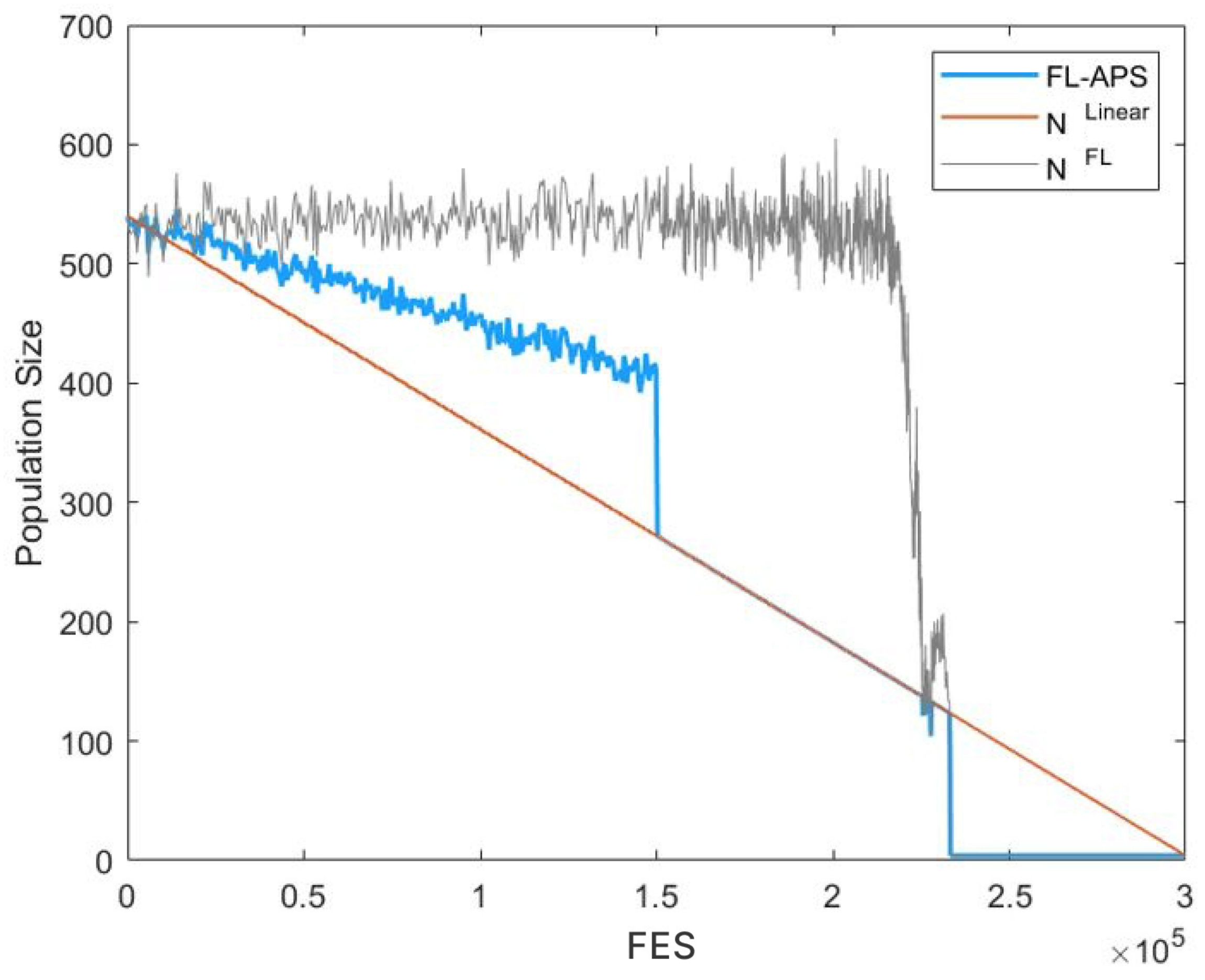
3.3. Adaptive Population Size Mechanism Based on Fitness Landscape (FL-APS)

In this part, a novel adaptive population size scheme based on fitness landscape is proposed to adjust the appropriate population size dynamically. As we all know, the LSHADE proposed linear population size reduction (LPSR) scheme has proven to be an outstanding scheme for population size adaptation. However, when the number of evaluations increases, the LPSR mechanism simply declines linearly and does not adjust to the different landscape of objective functions. That is why we proposed the adaptive population size scheme based on fitness landscape (FL-APS). The detail of proposed mechanism is given in Equation (15):

$$N_{G+1}^{FL}=round\left[\left(N^{init}-N^{min}\right)\times \phi +N^{min}\right]$$

(15)

where $N^{min}$ and $N^{init}$ denote the minimum and initial value of population size, and $N^{min}=4$ because DE/current-to-pcbest mutation operator requires at least four individuals. φ is the value of local fitness characteristics; when φ is close to 0, it is close to the unimodal local fitness landscape, N is close to $N^{min}$, and convergence is accelerated by a smaller value of N; when φ is close to 1, it is close to the multi-modal local fitness landscape, N is close to $N^{init}$, and N is large to maintain the population diversity. Therefore, the population size N can be adjusted adaptively by extracting fitness landscape characteristics each generation in the iterative process.

After introducing a FES_t into the FL-APS, a balance between population size and generation number could be achieved, and the FL-APS can be altered to Equation (16):

$$N_{G+1}=\left\{\begin{array}{l}round\left[(N_{G+1}^{FL}+N_{G+1}^{Linear}\right)/2], if FES<FE{S}_t\\ \min (N_{G+1}^{FL},N_{G+1}^{Linear}), otherwise\end{array}\right.$$

(16)

where $N_{G+1}^{Linear}$ is the LPSR mechanism calculated by Equation (8). At the early stage of iteration, the relationship between population size and the number of fitness evaluation is balanced by calculating the average value of $N_{G+1}^{FL}$ and $N_{G+1}^{Linear}$. It can not only maintain a relatively large population size for exploration but also avoid wasting too much computing resources in the early stage. At the later stage of iteration, the minimum values of $N_{G+1}^{FL}$ and $N_{G+1}^{Linear}$ are selected to accelerate exploitation and lead to rapid convergence. To better illustrate the advantages of FL-APS, Figure 1 shows the reduction curve of FLADE population size on f₆ benchmark function in CEC2014; the dimension number is set to D = 30, initial population size is set to $N^{init}=25\log \left(D\right)\sqrt{D}$, the minimum population size is set to N^min = 4, and the maximum number of function evaluations is set to FES_max = 10,000 D. The FL-APS with the FES_t = 1/2 ∗ FES_max is the default setting for the adaptation of population size. A more in-depth of the parameters of FL-APS will be discussed in Section 4.4. We can see from Figure 1 that the population size of FL-APS decreased more slowly than LPSR with the reduction of FES at the beginning of the evolution, which enables the population to maintain enough diversity to explore more areas in the early stage. In the last stage of the iteration, the population size decreased rapidly to accelerate the convergence as the fitness landscape characteristics φ decreased.

Figure 2 shows the number of generations of FL-APS and LSHADE on different types of CEC2014 functions. As can be seen from Figure 2, FL-APS can have more generations in the unimodal function to accelerate convergence, maintain a large population size in the multimodal function and hybrid function to maintain diversity, and adjust population size adaptively in the composition function according to the complexity of landscape fitness.

3.4. Complete Procedure of the Proposed FL-ADE

The parameters CR and F of FL-ADE are consistent with the parameter mechanism of LSHADE, the mutation strategy uses the proposed DE/current-to-pcbest/1, and the population size mechanism is FL-APS. The pseudocode of the proposed FL-ADE is presented in Algorithm 3. To better introduce the proposed FL-ADE, the specific operation is as follows:

• Step 1—Initialization: The initialization of FL-ADE is the same as in classic DE. Randomly initialize a population of N individuals $P^G=(x_{1,G},\dots ,x_{N,G})$ with $x_{i,G}=(x_{i,G}^1,x_{i,G}^2,\dots ,x_{i,G}^D)$, and each individual is uniformly distributed in the range [X_min, X_max] with $i=(1,2,\dots ,N)$ according to Equation (1). Set up the maximum generation number FE = 10,000 × D, the generation index G = 1, the initial population size $N^{init}=25\log \left(D\right)\sqrt{D}$, the minimum population size N^min = 4, and the percentage of top individuals in archive $cbest pc=0.03$. Set the other parameters to be the same as in LSHADE: H = 6, set all values in M_CR, M_F to 0.5, and archive A = ∅, as Line 1–Line 4 in Algorithm 3.
• Step 2—For each generation G, all individuals are re-indexed in ascending order of their distance with the best individual x_best,G. Then calculate the local fitness landscape feature value φ and the approximate local optimal individual archive cbest (Algorithm 2). Generating parameters F and CR with successful parameter memory M_CR and M_F is same as in LSHADE, where $rand{n}_i(\mu ,{\sigma }^2)$, $rand{c}_i(\mu ,{\sigma }^2)$ are values selected randomly from normal and Cauchy distribution with mean μ and variance σ² as in Lines 6–14 in Algorithm 3.
• Step 3—Mutation: Randomly choose one of the top p% individuals from the archive $cbest$ as $x_{cbest}^p$. Generate mutant vector $v_{i,G}$ via the DE/current-to-pcbest/1 according to Equation (13); then deal with infeasible solutions according to Equation (14), as stated in Lines 15–17 in Algorithm 3.
• Step 4—Crossover: Use the binomial crossover of the classical DE to generate the trial vector $u_{i,G}$ according to Equation (6).
• Step 5—Selection: As in classic DE, after comparing each target individual with the $x_{i,G}$ and $u_{i,G}$, the individual with better fitness value will enter the next generation, and the parameters CR and F are stored in the successful parameter archive $S_{CR}$ and $S_F$, as in Lines 18–28 in Algorithm 3.
• Step 6: Update memories $M_{CR}$ and $M_F$ according to Algorithm 1. Adaptively adjust population size according to Equation (16). Repeat step 3 to step 6 until the number of evaluations is greater than or equal to $FE{S}_{max}$, as in Lines 29–31 in Algorithm 3.

Algorithm 3: FL-ADE algorithm

Input: Bound constraints $\left[X_{min},X_{max}\right]$, the fixed maximum number of function evaluations $FE{S}_{max}$, benchmark functions $f\left(X\right)$; Output: Best fitness value $f\left(x_{best}\right)$, best individual $X_{best}$ // Initialization phase 1. $G=1, N_G=N^{init},$ Archive $A=\varnothing$; 2. Initialize population $P_G=\left(x_{1,G},\dots ,x_{N,G}\right)$ randomly; 3. Evaluate $P_G$, $FES=N_G;$; 4. Set all values in $M_{CR}, M_F$ to 0.5; // Main loop 5. While $FES<FE{S}_{max}$ do 6. $S_{CR}=\varnothing ,S_F=\varnothing ;$ 7. For $i=1$ to $N$ do 8.  $r_i=$ Select from $\left[1,H\right]$ randomly; 9.  If $M_{CR,r_I}=\perp$, $C{R}_{i,G}=0$. Otherwise 10.   $C{R}_{i,G}=rand{n}_i\left(M_{CR},ri, 0.1\right);$ 11.  $F_{i,G}=rand{c}_i\left(M_F,ri, 0.1\right);$ 12.  End If 13.  End For // Adaptively mixed mutation strategy 14.   Calculate $\phi$ and get the archive of $cbest$ (Algorithm 2); 15.  Dealing with infeasible solutions according to Equation (14); 16.  Randomly choose one of the top p% individuals from the archive $cbest$ as $x_{cbest}^p$; 17.  Generate trial vector $u_{i,G}$ according to DE/current-to-$pcbest$/1/bin in Equation (13); 18.  For $i=1$ to $N$ do 19. If $f\left(u_{i,G}\right)\le f\left(x_{i,G}\right)$ then 20.  $x_{i,G+1}=u_{i,G}$; 21.  Else 22.  $x_{i,G+1}=x_{i,G}$; 23.  End If 24.  If $f\left(u_{i,G}\right)<f\left(x_{i,G}\right)$ then 25.   $x_{i,G}\to A$; 26.   $C{R}_{i,G}\to S_{CR}$, $F_{i,G}\to S_F$; 27.  End If 28. End For 29. If necessary, delete randomly selected individuals from the archive such that the archive size is |A|. 30. Update memories $M_{CR}$ and $M_F$ (Algorithm 1); // FL-APS 31. Adaptively adjust population size according to Equation (16); 32. $G++;$ 33. End While

4. Experiment Analysis of FL-ADE Algorithm

In this section, we demonstrate the performance of FL-ADE through experimental results and discuss the influence of its components.

4.1. Experiment Environment

FL-ADE was tested on 30 benchmark test functions developed for IEEE CEC2014 listed in

Table 1. The benchmark functions of IEEE CEC2014.

Type	Func.	Functions	Search Range	$\mathit{f}\left({\mathit{x}}^{*}\right)$
Unimodal functions	$f_1$ $f_2$ $f_3$	Rotated high conditioned elliptic function	${\left[-100,100\right]}^{ D}$ ${\left[-100,100\right]}^{ D}$ $\left[-100,100\right]{ }^D$	100
		Rotated Bent Cigar function		200
		Rotated Discus function		300
Simple multimodal functions	$f_4$	Shifted and rotated Rosenbrock’s function	$\left[-100,100\right]{ }^D$	400
	$f_5$	Shifted and rotated Ackley’s function	$\left[-100,100\right]{ }^D$	500
	$f_6$	Shifted and rotated Weierstrass function	${\left[-100,100\right]}^{ D}$	600
	$f_7$	Shifted and rotated Griewank’s function	${\left[-100,100\right]}^{ D}$	700
	$f_8$	Shifted Rastrigin’s function	${\left[-100,100\right]}^{ D}$	800
	$f_9$	Shifted and rotated Rastrigin’s function	${\left[-100,100\right]}^{ D}$	900
	$f_{10}$	Shifted Schwefel’s function	${\left[-100,100\right]}^{ D}$	1000
	$f_{11}$	Shifted and rotated Schwefel’s function	${\left[-100,100\right]}^{ D}$	1100
	$f_{12}$	Shifted and rotated Katsuura function	$\left[-100,100\right]{ }^D$	1200
	$f_{13}$	Shifted and rotated HappyCat function	$\left[-100,100\right]{ }^D$	1300
	$f_{14}$	Shifted and rotated HGBat function	$\left[-100,100\right]{ }^D$	1400
	$f_{15}$	Shifted and rotated expanded Griewank’s plus Rosenbrock’s function	$\left[-100,100\right]{ }^D$	1500
	$f_{16}$	Shifted and rotated expanded Scaffer’s function	${\left[-100,100\right]}^{ D}$	1600
Hybrid functions	$f_{17}$	Hybrid function 1 (N = 3)	${\left[-100,100\right]}^{ D}$	1700
	$f_{18}$	Hybrid function 2 (N = 3)	${\left[-100,100\right]}^{ D}$	1800
	$f_{19}$	Hybrid function 3 (N = 4)	${\left[-100,100\right]}^{ D}$	1900
	$f_{20}$	Hybrid function 4 (N = 4)	${\left[-100,100\right]}^{ D}$	2000
	$f_{21}$	Hybrid function 5 (N = 5)	${\left[-100,100\right]}^{ D}$	2100
	$f_{22}$	Hybrid function 6 (N = 5)	${\left[-100,100\right]}^{ D}$	2200
Composition functions	$f_{23}$	Composition function 1 (N = 5)	$\left[-100,100\right]{ }^D$	2300
	$f_{24}$	Composition function 2 (N = 3)	$\left[-100,100\right]{ }^D$	2400
	$f_{25}$	Composition function 3 (N = 3)	$\left[-100,100\right]{ }^D$	2500
	$f_{26}$	Composition function 4 (N = 5)	$\left[-100,100\right]{ }^D$	2600
	$f_{27}$	Composition function 5 (N = 5)	$\left[-100,100\right]{ }^D$	2700
	$f_{28}$	Composition function 6 (N = 5)	$\left[-100,100\right]{ }^D$	2800
	$f_{29}$	Composition function 7 (N = 3)	$\left[-100,100\right]{ }^D$	2900
	$f_{30}$	Composition function 8 (N = 3)	$\left[-100,100\right]{ }^D$	3000

. For these benchmarks, they can be categorized into four groups:

(1)

Unimodal functions $f_1-f_3$.

(2)

Simple multimodal functions $f_4-f_{16}$.

(3)

Hybrid functions $f_{17}-f_{22}$.

(4)

Composition functions $f_{23}-f_{30}$.

The performance of an algorithm is estimated by the fitness error $\Delta f=f-f^{*}$ ($f$ was the best result obtained by the corresponding algorithm on a particular function, and $f^{*}$ is the global optimal of the function). If $\Delta f$ is smaller than $eps=10\times {10}^{-8}$ it is considered as $0$.

To demonstrate the efficiency of the proposed FL-ADE, seven high-performing state-of-art DE variants that appeared from 2011 to 2019 are selected in this research. The first competitor is EPSDE [45], which employed an ensemble of mutation strategies and control parameters. MPEDE [46] is the second algorithm to compare, which simultaneously consists of three mutation strategies. The third competitor is CoBiDE [47], in which the covariance matrix learning and the bimodal distribution parameters setting are incorporated into the DE framework. The fourth peer algorithm SHADE [22] uses a different parameter adaptation mechanism based on the success history to improve JADE [12]. The fifth contender is LSHADE [29], which enhances SHADE’s overall optimization performance by implementing a linear population size reduction technique, which helped LSHADE win the CEC2014 championship. The sixth competitor is the second place of the CEC2017 competition LSHADE_cnEpSin [40], which is an improved version of the first place of the CEC2016 competition LSHADE_EpSin [48]. The last comparison algorithm is PaDE [39], which proposes a novel control parameter adaptation schemes and a novel parabolic population size reduction scheme.

4.2. Parameter Settings of the Contrasted Algorithms

As previously stated, this paper compares seven DE variants: EPSDE, MPEDE, SHADE, LSHADE, LSHADE cnEpSin, PaDE, and the newly proposed FL-ADE algorithm. All these algorithms adopted the recommended parameter settings of the cited references in our experiments as summarized in

Table 2. Recommended parameter settings of all these contrasted algorithms.

No.	Algorithms	Parameters Initial Settings
1	EPSDE [45]	$F=\left[0.4,0.9\right]$$, CR=\left[0.1,0.9\right]$$, N=50$;
2	MPEDE [46]	$F\sim C\left(\mu F, 0.1\right), \mu F=0.5$$, Cr\sim N\left(\mu Cr, 0.1\right)$$, \mu Cr=0.5$$, N=250$$, c=0.1$$, p=0.05$$, {\lambda }_1={\lambda }_2={\lambda }_3=0.2$$, ng=20$;
3	CoBiDE [47]	$N=60$$, pb=0.4$$, ps=0.5$;
4	SHADE [22]	$F\sim C\left(\mu F, 0.1\right)$$, \mu F=0.5$$, Cr\sim N\left(\mu Cr, 0.1\right)$$, \mu Cr=0.5$$, N=100$$, p=0.2$$, H=100$;
5	LSHADE [29]	$F\&Cr$$\mathrm{same} \mathrm{as} \mathrm{SHADE}, N=18D\sim 4$$, r^{arc}=2.6$$, p =0.11$$, H=6$;
6	LSHADE_cnEpSin [40]	$\mu F=0.5$$, \mu Cr=0.5$$, \mu Freq=0.5$$, ps=0.5$$, pc=0.4$$, \mathrm{H} = 5; N=18D\sim 4$$, r^{arc}=1.4$$, p=0.11$;
7	PaDE [39]	$\mu F=0.8$$, \mu Cr=0.6$$, F\&Cr$$\mathrm{same} \mathrm{as} \mathrm{LSHADE}, k=4$$, p=0.11$$, N =25log\left(D\right)\sqrt{D}\sim 4$$, r^{arc}=1.6$$, T_0=70$$, r^d=0.04$$, H=4$;
8	FL-ADE	$F\&Cr\&H\&r^{arc}$$\mathrm{same} \mathrm{as} \mathrm{LSHADE}, N=25log\left(D\right)\sqrt{D}\sim 4$$, pc=0.3$, $FE{S}_t=\left(1/2\right)\ast FE{S}_{max}$.

.

In EPSDE, the population size $N=50$ is maintained constant, the pool of crossover rate $CR$ values is taken in the range 0.1–0.9 in steps of 0.1, and the pool of scale factor $F$ values is taken in the range 0.4–0.9 in steps of 0.1.

In MPEDE, the population size is set to $N=250$, and the two newly introduced ones, namely the ratio ${\lambda }_1$ (as ${\lambda }_1={\lambda }_2={\lambda }_3$) between indicator population and whole population, are set to ${\lambda }_1={\lambda }_2={\lambda }_3=0.2$, and generation gap $ng$ for determining the recent best performing mutation strategy periodically is set to $ng=20$. The scale factor $F$ obeys semifixed Cauchy distribution, $F\sim C\left(\mu F, 0.1\right)$, and $\mu F$ is the location parameter with its initial value is equal to 0.5. The crossover rate $CR$ obeys semifixed Normal distribution, $Cr\sim N\left(\mu Cr, 0.1\right)$, $\mu Cr$ denotes the mean value, $\mu Cr$ denotes the mean value, and the initial value of $\mu Cr$ is set to $\mu Cr=0.5$. The ratio of top superior individuals $p=0.05$, and balance parameter $c=0.1$.

In CoBiDE the population size $N=60$, $pb=0.4$ denotes the probability to execute DE according to the covariance matrix learning, and $ps=0.5$ denotes the proportion of the individuals chosen from the current population to calculate the covariance matrix.

In SHADE, the control parameter settings of $F$ and $CR$ are the same as MPEDE, the population size $N=100$, and the ratio of top superior individuals $p=0.2$. Moreover, historical success values of $F$ and $Cr$ are recorded in a H-entry pool in SHADE, where $H=100$.

LSHADE employs the same initial values and distributions of control parameters $F$ and $Cr$ as SHADE, and a linear population size reduction scheme is also employed in LSHADE with the initial population size equaling to $N=18\times D$, and the minimum population size is equal to 4. Furthermore, the parameter $r^{arc}=2.6$, defining the factor of external archive size; the parameter $H=6$, defining entry number in the memory pool; and the parameter $p=0.11$, denoting the ratio of top superior individuals, are also different from the ones in SHADE.

In LSHADE_cnEpSin, the crossover operator is performed based on the covariance matrix learning with Euclidean neighborhood with a probability $pc=0.4$, and $ps=0.5$ is the proportion of individuals that are used to generate the covariance matrix; $ufreq$ represents the mean frequency of the sinusoidal function is set to 0.5. The initial values of all $\mu F$, $\mu CR$ are both set to 0.5, the initial population size equaling to $N=18\times D$, the minimum population size is equal to 4, the factor of external archive size $r^{arc}=1.4$, the entry number in the memory pool $H=5$, and the ratio of top superior individuals $p=0.11$.

In PaDE, control parameters $F$ and $Cr$ obey Cauchy distribution $C\left(\mu F , 0.1\right)$ and Normal distribution $N\left(\mu Cr, 0.1\right)$, respectively, and the initial values of $\mu F$ and $\mu Cr$ are set to $\mu F=0.8$ and $\mu Cr=0.6$. The initial population size is set to $N=25\log \left(D\right)\sqrt{D}$. All individuals in the PaDE algorithm are categorized into $k$ groups, and $k$ is set to a constant value, $k=4$. Moreover, a time stamp scheme is employed in the external archive, and the timestamp threshold is set to $T0=70$. Parameters $r^{arc}$ and $p$ are set tuned values under the time stamp scheme, $r^{arc}=1.6$ and $p=0.11$, and the default setting of decay rate $r^d$ is a fixed constant value $r^d=0.04$.

In the proposed FL-ADE algorithm, the parameter $F\&Cr\&H\&r^{arc}$ is consistent with LSHADE, the initial population size $N=25\log \left(D\right)D\surd$ and the minimum population size equaling to 4. The ratio of top superior individuals in archive $cbest$ is set to $pc=0.3$; the threshold $FE{S}_t=\left(1/2\right)\ast FE{S}_{max}$.

4.3. Comparison with State-of-the-Art DE Algorithms

In this section, the proposed FL-ADE was compared with the seven of DE variants: EPSDE [45], MPEDE [46], CoBiDE [47], SHADE [22], LSHADE [29], LSHADE_cnEpSin [40], and PaDE [39]. The experiments are conducted on $f_1-f_{30}$ benchmarks of CEC2014 on 10-D, 30D, and 50D optimization, respectively. The allowed maximum number of function evaluations ($FE{S}_{max}$) of each run was set to 10,000 $\times$ D (D is the dimension of the problem) based on the guideline provided in the special session of CEC2014 [31], and 51 runs were conducted on each benchmark.

Figure 3, Figure 4 and Figure 5 summarize the comparison results between FL-ADE and other DE algorithms, while the detailed comparison results are shown in

Table 3. Comparison results between EPSDE, MPEDE, CoBiDE, SHADE, LSHADE, LSHADE-cnEpSin, PaDE, and FL-ADE on 10D functions.

D = 10	EPSDE [45]	MPEDE [46]	CoBiDE [47]	SHADE [22]	LSHADE [29]	LASHDE_cnEpSin [40]	PaDE [39]	FL-ADE
$f_1$	0.00E+00 (0.00E+00) =	0.00E+00 (0.00E+00) =	0.00E+00 (0.00E+00) =	0.00E+00 (0.00E+00) =	0.00E+00 (0.00E+00) =	0.00E+00 (0.00E+00) =	0.00E+00 (0.00E+00) =	0.00E+00 (0.00E+00)
$f_2$	0.00E+00 (0.00E+00) =	0.00E+00 (0.00E+00) =	0.00E+00 (0.00E+00) =	0.00E+00 (0.00E+00) =	0.00E+00 (0.00E+00) =	0.00E+00 (0.00E+00) =	0.00E+00 (0.00E+00) =	0.00E+00 (0.00E+00)
$f_3$	0.00E+00 (0.00E+00) =	0.00E+00 (0.00E+00) =	0.00E+00 (0.00E+00) =	0.00E+00 (0.00E+00) =	0.00E+00 (0.00E+00) =	0.00E+00 (0.00E+00) =	0.00E+00 (0.00E+00) =	0.00E+00 (0.00E+00)
$f_4$	7.82E−02 (5.58E−01)−	1.46E+01 (1.71E+01)−	7.75E+00 (1.36E+01)−	2.28E+01 (1.65E+01)−	2.33E+01 (1.64E+01) −	1.77E+01 (1.06E+01)−	2.59E+01 (1.53E+01)−	3.34E+01 (6.82E+00)
$f_5$	2.00E+01 (1.43E−02)+	1.12E+01 (9.28E+00) =	1.96E+01 (2.34E+00)+	1.66E+01 (6.38E+00)+	1.64E+01 (6.88E+00) =	1.36E+01 (8.89E+00) =	1.25E+01 (8.73E+00) =	1.37E+01 (8.98E+00)
$f_6$	2.86E+00 (5.95E−01)+	0.00E+00 (0.00E+00) =	4.82E−06 (1.47E−05)+	2.75E−04 (1.19E−03)+	1.44E−01 (2.13E−01)+	0.00E+00 (0.00E+00) =	0.00E+00 (0.00E+00) =	0.00E+00 (0.00E+00)
$f_7$	1.46E−02 (9.01E−03)+	0.00E+00 (0.00E+00)−	2.83E−02 (2.03E−02)+	2.53E−03 (2.33E−03)+	3.38E−04 (1.71E−03) =	1.45E−04 (1.04E−03) =	1.66E−03 (4.47E−03) =	1.25E−03 (5.19E−03)
$f_8$	0.00E+00 (0.00E+00) =	0.00E+00 (0.00E+00) =	0.00E+00 (0.00E+00) =	0.00E+00 (0.00E+00) =	0.00E+00 (0.00E+00) =	0.00E+00 (0.00E+00) =	0.00E+00 (0.00E+00) =	0.00E+00 (0.00E+00)
$f_9$	4.13E+00 (1.07E+00)+	1.71E+00 (7.75E−01)+	4.04E+00 (1.52E+00)	3.22E+00 (8.70E−01)+	3.66E+00 (1.05E+00)+	1.85E+00 (6.90E−01)+	2.09E+00 (9.60E−01)+	4.68E−01 (8.53E−01)
$f_{10}$	3.18E−02 (4.02E−02) =	0.00E+00 (0.00E+00)−	1.02E−02 (3.08E−02)+	1.22E−03 (8.75E−03)−	1.22E−03 (8.75E−03)−	1.22E−03 (8.75E−03)−	4.90E−03 (1.70E−02)−	1.71E−02 (3.08E−02)
$f_{11}$	3.49E+02 (1.07E+02)+	4.97E+01 2.29E+01)+	7.75E+01 (8.29E+01)+	1.15E+02 (8.84E+01)+	5.13E+01 (4.75E+01)+	2.33E+01 (3.11E+01) =	2.37E+01 (3.03E+01) =	1.49E+01 (1.31E+01)
$f_{12}$	3.24E−01 (5.99E−02)+	1.99E−01 (4.09E−02)+	3.41E−01 (1.76E−01)+	1.81E−01 (3.00E−02)+	8.41E−02 (2.41E−02)+	6.78E−02 (1.74E−02) =	9.57E−02 (2.92E−02)+	6.91E−02 (2.26E−02)
$f_{13}$	1.26E−01 (2.42E−02)+	7.17E−02 (1.88E−02)+	1.11E−01 (4.81E−02)+	1.06E−01 (1.72E−02)+	5.64E−02 (1.62E−02)+	4.65E−02 (1.12E−02)+	4.84E−02 (1.59E−02)+	4.04E−02 (1.37E−02)
$f_{14}$	1.31E−01 (4.19E−02)+	1.21E−01 (3.16E−02)+	1.35E−01 (3.70E−02)+	1.20E−01 (3.61E−02)+	6.91E−02 (1.80E−02)−	8.46E−02 (3.48E−02) =	7.97E−02 (2.80E−02) =	8.14E−02 (2.70E−02)
$f_{15}$	7.37E−01 (1.18E−01)+	4.58E−01 (9.13E−02)+	6.18E−01 (2.37E−01)+	5.21E−01 (9.76E−02)+	3.90E−01 (9.10E−02) =	3.81E−01 (6.82E−02) =	3.87E−01 (8.09E−02) =	3.73E−01 (7.06E−02)
$f_{16}$	2.57E+00 (2.32E−01)+	1.29E+00 (2.45E−01)+	2.01E+00 (5.10E−01)+	1.71E+00 (3.19E−01)+	1.55E+00 (2.80E−01)+	1.03E+00 (2.92E−01)+	1.13E+00 (3.00E−01)+	8.18E−01 (2.64E−01)
$f_{17}$	5.47E+01 (7.23E+01)+	1.05E+00 (2.36E+00) =	3.82E−01 (3.84E−01) =	1.16E+00 (2.01E+00) =	1.50E+00 (1.10E+00)+	2.58E+01 (4.01E+01)+	1.59E+00 (1.84E+00)+	7.43E−01 (7.87E−01)
$f_{18}$	1.26E+00 (8.96E−01)+	3.83E−02 (1.41E−01)−	5.86E−02 (1.95E−01)−	1.21E−01 (1.29E−01) =	2.16E−01 (1.79E−01) =	3.46E−01 (4.68E−01) =	8.78E−02 (9.66E−02)−	1.76E−01 (1.81E−01)
$f_{19}$	1.43E+00 (2.27E−01)+	7.90E−02 (2.65E−02)+	2.82E−01 (1.17E−01)+	1.67E−01 (7.76E−02)+	1.59E−01 (7.47E−02)+	3.58E−01 (4.43E−01)+	5.09E−02 (2.47E−02) =	5.61E−02 (2.96E−02)
$f_{20}$	1.62E−01 (8.75E−02) =	5.72E−02 (3.52E−02)−	3.09E−02 (5.17E−02)−	2.61E−01 (7.59E−02)+	1.64E−01 (7.96E−02)+	2.70E−01 (2.00E−01) =	1.22E−01 (9.60E−02) =	1.69E−01 (1.57E−01)
$f_{21}$	2.39E+00 (4.42E+00)+	7.37E−02 (8.89E−02)−	1.05E−01 (1.58E−01)−	2.11E−01 (1.96E−01) =	2.01E−01 (1.63E−01) =	1.52E+00 (4.01E+00)+	2.51E−01 (2.43E−01) =	3.22E−01 (2.58E−01)
$f_{22}$	2.01E+01 (1.11E+00)+	9.14E−02 (2.06E−02)+	6.89E−01 (7.69E−01)+	1.10E−01 (3.56E−02) =	1.49E−01 (6.33E−02)+	1.60E+00 (4.91E+00)+	7.67E−02 (2.56E−02)−	1.05E−01 (4.25E−02)
$f_{23}$	3.29E+02 (2.87E−13) =	3.29E+02 (2.87E−13)+	3.29E+02 (2.87E−13) =	3.29E+02 (2.87E−13) =	3.29E+02 (2.87E−13) =	3.29E+02 2.87E−13) =	3.29E+02 (2.87E−13) =	3.29E+02 (2.87E−13)
$f_{24}$	1.12E+02 (1.72E+00)+	1.03E+02 (3.52E+00)−	1.11E+02 (2.85E+00)+	1.09E+02 (1.97E+00)+	1.10E+02 (1.55E+00)+	1.07E+02 (1.79E+00) =	1.07E+02 (3.06E+00) =	1.07E+02 (2.11E+00)
$f_{25}$	1.91E+02 (2.54E+01)+	1.14E+02 (7.52E+00)+	1.27E+02 (3.00E+01)+	1.19E+02 (4.53E+00)+	1.30E+02 (3.43E+01)+	1.24E+02 (2.04E+01)+	1.13E+02 (1.21E+01)+	1.10E+02 (1.34E+01)
$f_{26}$	1.00E+02 (2.66E−02)+	1.00E+02 (2.22E−02)+	1.00E+02 (4.49E−02)+	1.00E+02 (2.00E−02)+	1.00E+02 (1.32E−02)+	1.00E+02 (1.22E−02) =	1.00E+02 (1.95E−02) =	1.00E+02 (1.78E−02)
$f_{27}$	3.40E+02 (1.32E+02)+	9.46E+00 (5.58E+01)+	7.64E+01 (1.53E+02)+	7.48E+01 (1.42E+02)+	2.32E+01 (8.75E+01)+	1.40E+02 (1.71E+02)+	3.85E+01 (1.14E+02)+	4.81E+01 (1.20E+02)
$f_{28}$	3.06E+02 (1.17E−02)−	3.67E+02 (1.42E+01)−	3.60E+02 (1.41E+01)−	3.85E+02 (4.16E+01)−	3.67E+02 (5.52E+00)−	3.80E+02 (2.95E+01) =	3.90E+02 (5.04E+01)−	3.80E+02 (3.08E+01)
$f_{29}$	2.02E+02 (4.50E−01)−	2.22E+02 (7.97E−02)−	2.18E+02 (1.77E+01)−	2.20E+02 (1.27E+01) =	2.22E+02 (5.26E−01)−	2.22E+02 (5.65E−01) =	2.22E+02 (1.93E−01)−	2.22E+02 (5.61E−01)
$f_{30}$	2.33E+02 (5.35E+00)−	4.64E+02 (1.24E+01)=	4.63E+02 (5.24E+00)+	4.70E+02 (1.72E+01)+	4.63E+02 (5.22E+00)=	4.70E+02 (1.83E+01)=	4.66E+02 (1.14E+01)+	4.66E+02 (1.18E+01)
+/=/−	19/7/4	11/10/9	18/6/6	17/10/3	14/11/5	9/19/2	8/16/6	−/−/−

,

Table 4. Comparison results between EPSDE, MPEDE, CoBiDE, SHADE, LSHADE, LSHADE-cnEpSin, PaDE, and FL-ADE on 30D functions.

D = 30	EPSDE [45]	MPEDE [46]	CoBiDE [47]	SHADE [22]	LSHADE [29]	LASHDE_cnEpSin [40]	PaDE [39]	FL-ADE
$f_1$	1.10E+04 (2.17E+04)+	3.82E+01 (1.89E+02)+	1.43E+04 (1.24E+04)+	1.60E+03 (2.29E+03)+	0.00E+00 (0.00E+00) =	0.00E+00 (0.00E+00) =	0.00E+00 (0.00E+00) =	0.00E+00 (0.00E+00)
$f_2$	0.00E+00 (0.00E+00) =	0.00E+00 (0.00E+00)+	0.00E+00 (0.00E+00) =	0.00E+00 (0.00E+00) =	0.00E+00 (0.00E+00) =	0.00E+00 (0.00E+00) =	0.00E+00 (0.00E+00) =	0.00E+00 (0.00E+00)
$f_3$	0.00E+00 (0.00E+00) =	0.00E+00 (0.00E+00)+	0.00E+00 (0.00E+00) =	0.00E+00 (0.00E+00) =	0.00E+00 (0.00E+00) =	0.00E+00 (0.00E+00) =	0.00E+00 (0.00E+00) =	0.00E+00 (0.00E+00)
$f_4$	3.57E+00 (2.44E+00)+	3.16E−04 (1.29E−03)+	9.70E−06 (3.46E−05)+	0.00E+00 (0.00E+00) =	0.00E+00 (0.00E+00) =	0.00E+00 (0.00E+00) =	0.00E+00 (0.00E+00) =	0.00E+00 (0.00E+00)
$f_5$	2.03E+01 (3.82E−02)+	2.04E+01 (3.65E−02)+	2.03E+01 (2.63E−01) =	2.02E+01 (2.55E−02)+	2.01E+01 (2.83E−02)+	2.01E+01 (3.27E−02)+	2.02E+01 (4.42E−02)+	2.01E+01 (3.07E−02)
$f_6$	1.89E+01 (1.69E+00)+	2.08E+00 (1.63E+00)+	1.18E+00 (1.11E+00)+	6.02E+00 (3.88E+00)+	8.61E+00 (2.90E+00)+	2.63E−06 (7.26E−06)−	0.00E+00 (0.00E+00)−	1.97E−01 (5.06E−01)
$f_7$	1.16E−03 (4.30E−03)+	1.06E−03 (4.12E−03)+	0.00E+00 (0.00E+00) =	3.87E−04 (1.93E−03) =	0.00E+00 (0.00E+00) =	0.00E+00 (0.00E+00) =	0.00E+00 (0.00E+00) =	0.00E+00 (0.00E+00)
$f_8$	0.00E+00 (0.00E+00) =	0.00E+00 (0.00E+00)+	0.00E+00 (0.00E+00) =	0.00E+00 (0.00E+00) =	0.00E+00 (0.00E+00) =	0.00E+00 (0.00E+00) =	0.00E+00 (0.00E+00) =	0.00E+00 (0.00E+00)
$f_9$	4.27E+01 (6.94E+00)+	3.15E+01 (8.16E+00)+	3.97E+01 (1.11E+01)+	2.24E+01 (3.57E+00)+	1.16E+01 (2.06E+00)+	1.34E+01 (2.47E+00)+	8.30E+00 (1.57E+00)+	5.21E+00 (1.97E+00)
$f_{10}$	1.25E+00 (7.65E+00)+	2.24E+01 (3.69E+00)+	5.78E+01 (1.31E+01)+	4.49E−03 (8.65E−03) =	2.48E−03 (6.78E−03)+	3.66E−03 (9.15E−03)+	1.22E−03 (4.95E−03) =	4.08E−03 (1.02E−02)
$f_{11}$	3.54E+03 (4.02E+02)+	2.94E+03 (3.02E+02)+	1.69E+03 (3.79E+02)+	1.80E+03 (1.81E+02)+	1.34E+03 (1.92E+02)+	1.26E+03 (2.07E+02)+	1.21E+03 (1.82E+02) =	1.17E+03 (1.88E+02)
$f_{12}$	5.03E−01 (6.24E−02)+	5.84E−01 (7.76E−02)+	2.56E−01 (3.26E−01)−	2.42E−01 (2.93E−02)+	1.77E−01 (2.81E−02)+	1.92E−01 (2.76E−02)+	1.83E−01 (2.77E−02)+	1.49E−01 (2.21E−02)
$f_{13}$	2.56E−01 (3.74E−02)+	2.03E−01 (3.01E−02)+	2.50E−01 (5.49E−02)+	2.23E−01 (3.30E−02)+	1.46E−01 (2.21E−02)+	1.35E−01 (1.59E−02)+	1.08E−01 (1.54E−02)+	9.53E−02 (1.26E−02)
$f_{14}$	2.96E−01 (8.06E−02)+	2.06E−01 (2.80E−02) =	2.36E−01 (3.68E−02)+	2.28E−01 (2.99E−02)+	2.14E−01 (2.65E−02) =	1.87E−01 (2.45E−02)−	2.23E−01 (2.17E−02) =	2.15E−01 (2.86E−02)
$f_{15}$	5.45E+00 (7.70E−01)+	4.83E+00 (9.71E−01)+	3.08E+00 (7.71E−01)+	3.10E+00 (4.66E−01)+	2.57E+00 (5.19E−01)+	2.31E+00 (2.57E−01)+	2.17E+00 (2.47E−01) =	2.11E+00 (2.74E−01)
$f_{16}$	1.11E+01 (3.22E−01)+	1.05E+01 (2.87E−01)+	9.84E+00 (7.78E−01)+	9.67E+00 (3.59E−01)+	9.11E+00 (3.53E−01)+	8.43E+00 (4.71E−01) =	8.48E+00 (3.98E−01) =	8.40E+00 (4.01E−01)
$f_{17}$	5.19E+04 (5.95E+04)+	7.51E+02 (3.08E+02)+	2.78E+02 (1.94E+02) =	9.90E+02 (3.13E+02)+	1.77E+02 (7.68E+01)−	1.26E+02 (8.76E+01)−	1.66E+02 (9.89E+01)−	2.62E+02 (1.09E+02)
$f_{18}$	2.55E+02 (4.50E+02)+	5.91E+01 (1.02E+01)+	1.14E+01 (4.38E+00)+	6.70E+01 (2.63E+01)+	4.40E+00 (1.76E+00) =	6.97E+00 (2.48E+00)+	5.31E+00 (2.42E+00) =	4.38E+00 (2.15E+00)
$f_{19}$	1.29E+01 (9.99E−01)+	4.20E+00 (6.85E−01)+	2.87E+00 (4.65E−01)−	4.58E+00 (7.68E−01)+	3.40E+00 (6.01E−01)−	2.75E+00 (6.37E−01)−	3.43E+00 (5.76E−01)−	3.88E+00 (7.01E−01)
$f_{20}$	4.86E+01 (4.87E+01)+	1.29E+01 (6.46E+00)+	7.55E+00 (3.20E+00)+	1.25E+01 (6.18E+00)+	3.95E+00 (7.84E−01)+	2.03E+00 (9.54E−01)−	2.66E+00 (1.11E+00) =	2.62E+00 (1.19E+00)
$f_{21}$	1.24E+04 (1.79E+04)+	1.91E+02 (8.70E+01)+	1.18E+02 (1.05E+02) =	2.43E+02 (1.28E+02)+	9.82E+01 (7.02E+01) =	8.04E+01 (8.75E+01) =	7.82E+01 (7.80E+01) =	1.01E+02 (8.46E+01)
$f_{22}$	2.24E+02 (9.80E+01)+	1.21E+02 (5.40E+01)+	1.21E+02 (8.90E+01)+	1.46E+02 (5.79E+01)+	2.92E+01 (8.71E+00)+	6.16E+01 (5.54E+01)+	6.84E+01 (5.34E+01)+	2.97E+01 (2.48E+01)
$f_{23}$	3.14E+02 (9.56E−13)−	3.15E+02 (4.02E−13) =	3.15E+02 (4.02E−13) =	3.15E+02 (4.02E−13) =	3.15E+02 (4.02E−13) =	3.15E+02 (1.25E−01)−	3.15E+02 (3.18E−13) =	3.15E+02 (4.02E−13)
$f_{24}$	2.29E+02 (6.01E+00)+	2.24E+02 (2.02E+00)+	2.23E+02 (1.10E+00)+	2.25E+02 (3.15E+00)+	2.23E+02 (1.32E+00)+	2.08E+02 (1.04E+01)−	2.24E+02 (1.18E+00)+	2.01E+02 (5.15E+00)
$f_{25}$	2.00E+02 (6.29E−01)+	2.01E+02 (2.21E+00)−	2.03E+02 (3.91E−01)+	2.08E+02 (2.54E+00)+	2.03E+02 (3.20E−02)+	2.03E+02 (3.81E−02)+	2.03E+02 (1.43E−01)+	2.00E+02 (5.09E−01)
$f_{26}$	1.00E+02 (4.83E−02)+	1.00E+02 (3.19E−02)+	1.00E+02 (4.72E−02)+	1.00E+02 (3.24E−02)+	1.00E+02 (1.82E−02)+	1.00E+02 (1.51E−02)+	1.00E+02 (1.40E−02)+	1.00E+02 (1.33E−02)
$f_{27}$	8.38E+02 (1.04E+02)+	3.62E+02 (4.20E+01)+	3.78E+02 (4.21E+01)+	3.38E+02 (4.39E+01)+	3.00E+02 (4.94E−05) =	3.00E+02 (1.85E−13)−	3.00E+02 (1.77E−13)−	3.00E+02 (1.83E+00)
$f_{28}$	3.97E+02 (1.37E+01)−	8.70E+02 (3.20E+01)+	8.18E+02 (2.83E+01)−	8.11E+02 (3.65E+01)−	8.26E+02 (2.03E+01)−	8.31E+02 (1.42E+01)−	8.60E+02 (1.41E+01)+	8.44E+02 (1.76E+01)
$f_{29}$	2.14E+02 (1.40E+00)−	7.00E+02 (9.77E+01)+	5.99E+02 (2.26E+02) =	7.25E+02 (1.15E+01)+	7.16E+02 (2.99E+00) =	7.20E+02 (5.28E+00)+	6.94E+02 (1.13E+02)+	7.17E+02 (4.49E+00)
$f_{30}$	5.77E+02 (1.44E+02)−	6.61E+02 (1.73E+02)−	7.07E+02 (2.16E+02)−	1.26E+03 (3.80E+02)=	1.79E+03 (7.80E+02)+	1.06E+03 (2.88E+02)=	5.99E+02 (2.27E+02)−	1.18E+03 (4.30E+02)
+/=/−	23/3/4	26/2/2	17/9/4	21/8/1	15/12/3	12/9/9	10/15/5	-/-/-

and

Table 5. Comparison results between EPSDE, MPEDE, CoBiDE, SHADE, LSHADE, LSHADE-cnEpSin, PaDE, and FL-ADE on 50D functions.

D = 50	EPSDE [45]	MPEDE [46]	CoBiDE [47]	SHADE [22]	LSHADE [29]	LASHDE_cnEpSin [40]	PaDE [39]	FL-ADE
$f_1$	2.28E+06 (5.96E+06)+	2.80E+05 (1.23E+05)+	3.05E+05 (1.27E+05)+	2.19E+04 (1.01E+04)+	1.37E+03 (1.42E+03) =	0.00E+00 (0.00E+00)−	4.11E+02 (5.63E+02)−	2.18E+03 (2.24E+03)
$f_2$	1.38E−08 (1.90E−08)+	6.23E+01 (3.17E+02)+	1.72E−01 (4.28E−01)+	0.00E+00 (0.00E+00) =	0.00E+00 (0.00E+00) =	0.00E+00 (0.00E+00) =	0.00E+00 (0.00E+00) =	0.00E+00 (0.00E+00)
$f_3$	2.20E−04 (1.06E−03)+	3.82E+00 (6.59E+00)+	5.81E−03 (8.13E−03)+	9.37E−08 (2.76E−07)+	0.00E+00 (0.00E+00) =	0.00E+00 (0.00E+00) =	0.00E+00 (0.00E+00) =	0.00E+00 (0.00E+00)
$f_4$	3.21E+01 (2.04E+01) =	5.84E+01 (3.42E+01) =	5.04E+01 (4.04E+01) =	1.09E+01 (2.95E+01)−	5.84E+01 (4.54E+01) =	4.66E+01 (3.75E+01)−	1.18E+01 (3.18E+01)−	5.59E+01 (4.89E+01)
$f_5$	2.06E+01 (6.49E−02)+	2.06E+01 (3.52E−02)+	2.02E+01 (3.37E−01)−	2.03E+01 (2.45E−02)+	2.03E+01 (2.89E−02)+	2.03E+01 (3.52E−02)+	2.03E+01 (6.28E−02)+	2.02E+01 (3.03E−02)
$f_6$	4.57E+01 (2.46E+00)+	1.11E+01 (2.85E+00)+	4.30E+00 (2.36E+00)+	8.53E+00 (4.90E+00)+	4.27E+00 (8.13E+00) =	1.05E−02 (7.26E−02)−	9.10E−02 (2.78E−01)−	9.89E−01 (1.08E+00)
$f_7$	7.63E−03 (9.81E−03)+	4.11E−03 (5.66E−03)+	0.00E+00 (0.00E+00) =	3.24E−03 (4.53E−03)+	0.00E+00 (0.00E+00) =	0.00E+00 (0.00E+00) =	0.00E+00 (0.00E+00) =	1.45E−04 (1.04E−03)
$f_8$	3.90E−02 (1.95E−01)+	1.05E+01 (1.73E+00)+	5.07E−09 (2.98E−08) =	0.00E+00 (0.00E+00) =	1.96E−07 (2.08E−07)+	3.36E−08 (2.54E−08)+	0.00E+00 (0.00E+00) =	0.00E+00 (0.00E+00)
$f_9$	1.48E+02 (1.86E+01)+	8.74E+01 (2.67E+01)+	8.35E+01 (2.22E+01)+	4.96E+01 (7.18E+00)+	1.98E+01 (2.68E+00)+	2.79E+01 (7.30E+00)+	1.59E+01 (2.14E+00)+	1.49E+01 (5.40E+00)
$f_{10}$	7.05E+02 (6.65E+02)+	4.52E+02 (4.86E+01)+	2.70E+02 (6.45E+01)+	5.88E−03 (8.04E−03)−	7.55E−01 (4.37E−01)+	1.25E+00 (5.40E−01)+	1.11E−02 (1.19E−02)−	9.32E−03 (8.60E−03)
$f_{11}$	8.98E+03 (4.95E+02)+	7.57E+03 (3.03E+02)+	4.04E+03 (7.13E+02)+	3.93E+03 (4.04E+02)+	3.60E+03 (3.78E+02)+	3.26E+03 (3.38E+02)+	3.18E+03 (3.28E+02) =	3.10E+03 (3.09E+02)
$f_{12}$	8.61E−01 (1.38E−01)+	8.86E−01 (8.62E−02)+	8.33E−02 (8.03E−02)−	2.39E−01 (2.99E−02)+	2.26E−01 (2.68E−02)+	2.60E−01 (3.67E−02)+	2.19E−01 (3.96E−02)+	1.88E−01 (2.81E−02)
$f_{13}$	3.73E−01 (5.19E−02)+	3.77E−01 (4.02E−02)+	3.50E−01 (5.53E−02)+	3.25E−01 (4.23E−02)+	1.98E−01 (2.30E−02)+	2.11E−01 (2.21E−02)+	1.71E−01 (2.24E−02)+	1.52E−01 (1.87E−02)
$f_{14}$	3.31E−01 (6.28E−02)+	2.93E−01 (2.53E−02)−	2.66E−01 (3.07E−02)−	2.92E−01 (2.86E−02)−	2.68E−01 (2.14E−02)−	1.86E−01 (2.29E−02)−	2.83E−01 (2.60E−02)−	3.09E−01 (2.39E−02)
$f_{15}$	1.82E+01 (2.18E+00)+	1.36E+01 (3.35E+00)+	5.98E+00 (1.29E+00)+	8.35E+00 (1.11E+00)+	6.11E+00 (9.60E−01)+	5.67E+00 (4.90E−01)+	5.02E+00 (4.84E−01) =	5.28E+00 (8.87E−01)
$f_{16}$	2.07E+01 (4.32E−01)+	1.97E+01 (3.61E−01)+	1.84E+01 (1.06E+00)+	1.81E+01 (4.20E−01)+	1.76E+01 (3.89E−01)+	1.69E+01 (3.94E−01)+	1.66E+01 (4.20E−01) =	1.66E+01 (5.08E−01)
$f_{17}$	2.19E+05 (1.31E+05)+	2.21E+03 (4.81E+02)+	1.07E+04 (7.97E+03)+	2.51E+03 (6.77E+02)+	1.05E+03 (3.42E+02)−	3.61E+02 (1.60E+02)−	1.64E+03 (4.27E+02) =	1.69E+03 (4.08E+02)
$f_{18}$	2.70E+03 (3.86E+03)+	1.05E+02 (1.93E+01)+	1.04E+02 (1.38E+02)−	1.38E+02 (3.24E+01)+	7.56E+01 (2.16E+01)−	1.98E+01 (5.08E+00)−	1.05E+02 (1.30E+01)+	9.42E+01 (1.37E+01)
$f_{19}$	2.47E+01 (1.17E+00)+	1.17E+01 (1.68E+00)+	6.82E+00 (1.10E+00)−	1.67E+01 (8.00E+00)+	1.05E+01 (9.70E−01)+	9.83E+00 (1.23E+00)+	7.99E+00 (2.04E+00) =	7.78E+00 (1.69E+00)
$f_{20}$	3.48E+02 (3.26E+02)+	1.22E+02 (6.22E+01)+	3.18E+01 (1.18E+01)+	2.01E+02 (5.32E+01)+	1.43E+01 (3.74E+00)+	6.16E+00 (1.92E+00)−	1.50E+01 (6.42E+00)+	9.57E+00 (2.71E+00)
$f_{21}$	6.48E+04 (5.11E+04)+	1.00E+03 (3.06E+02)+	2.50E+03 (2.54E+03)+	1.26E+03 (3.57E+02)+	4.36E+02 (1.07E+02) =	3.12E+02 (9.82E+01)−	5.67E+02 (1.70E+02)+	5.01E+02 (1.84E+02)
$f_{22}$	7.58E+02 (1.57E+02)+	5.37E+02 (1.67E+02)+	5.12E+02 (1.69E+02)+	4.51E+02 (1.46E+02)+	1.78E+02 (9.55E+01)+	8.20E+01 (5.88E+01) =	1.40E+02 (5.59E+01)+	9.22E+01 (6.00E+01)
$f_{23}$	3.37E+02 (2.50E−12)−	3.44E+02 (0.00E+00) =	3.44E+02 (4.11E−13)−	3.44E+02 (5.23E−13)−	3.44E+02 (4.86E−13)−	3.42E+02 (5.79E−01)−	3.44E+02 (4.89E−13)−	3.44E+02 (4.64E−13)
$f_{24}$	2.72E+02 (6.14E+00)+	2.71E+02 (6.89E+00)+	2.67E+02 (3.22E+00)+	2.75E+02 (2.19E+00)+	2.75E+02 (8.75E−01)+	2.68E+02 (1.50E+00)+	2.75E+02 (8.36E−01)+	2.30E+02 (3.01E+01)
$f_{25}$	2.02E+02 (3.96E+00)+	2.00E+02 (0.00E+00)+	2.07E+02 (1.13E+00)+	2.21E+02 (4.08E+00)+	2.05E+02 (2.47E−01)+	2.05E+02 (1.48E−01)+	2.06E+02 (4.57E−01)+	2.00E+02 (2.46E−13)
$f_{26}$	1.00E+02 (5.83E−02)+	1.24E+02 (4.27E+01)+	1.06E+02 (2.37E+01)+	1.04E+02 (1.95E+01)+	1.00E+02 (2.04E−02)+	1.00E+02 (2.87E−02)+	1.10E+02 (3.00E+01)+	1.04E+02 (1.96E+01)
$f_{27}$	1.57E+03 (4.19E+01)+	5.52E+02 (6.74E+01)+	4.18E+02 (6.37E+01)+	5.18E+02 (6.07E+01)+	3.30E+02 (3.01E+01)−	3.11E+02 (1.96E+01)−	3.11E+02 (2.33E+01)−	3.59E+02 (3.87E+01)
$f_{28}$	3.92E+02 (1.45E+01)−	1.20E+03 (4.86E+01)+	1.16E+03 (4.64E+01)+	1.17E+03 (4.87E+01)+	1.13E+03 (3.45E+01) =	1.15E+03 (2.86E+01)+	1.26E+03 (7.44E+01)+	1.13E+03 (3.01E+01)
$f_{29}$	2.25E+02 (2.41E+00)−	8.20E+02 (5.19E+01)+	1.11E+03 (2.12E+02)+	8.76E+02 (6.92E+01)+	7.24E+05 (5.16E+06)+	8.13E+02 (3.82E+01)+	6.03E+02 (1.18E+02)−	7.97E+02 (4.89E+01)
$f_{30}$	1.04E+03 (2.31E+02)−	9.54E+03 (8.16E+02)+	8.83E+03 (4.05E+02)=	9.96E+03 (7.85E+02)+	8.76E+03 (5.19E+02)=	8.27E+03 (4.84E+02)−	9.59E+03 (6.36E+02)+	8.88E+03 (5.31E+02)
+/=/−	25/1/4	27/2/1	20/4/6	24/2/4	16/9/5	15/4/11	13/9/8	-/-/-

. Table 3, Table 4 and Table 5 present the mean(std) (mean value and standard deviation) of fitness error for 51 runs of 10D, 30D, and 50D optimization, respectively. To have statistically sound conclusions, Wilcoxon rank-sum test is employed to show the differences between two algorithms on a single problem. The mean error and standard deviation (in bracket) of the function error values are provided in the tables. Three symbols “+, −, =” indicate that FL-ADE is significantly better than, significantly worse than, and almost the same as the corresponding competitor algorithm, respectively. The best result for each problem is shown in boldface. All of these are measured under Wilcoxon’s signed rand test with a significance level $\mathsf{\alpha }=0.05$.

Figure 3 summarizes the comparison results between FL-ADE and other DE algorithms on 10D, while the detailed comparison results are shown in Table 3. Table 3 shows that all contrasting methods perform equally well on benchmarks $f_1$, $f_2$, $f_3$, $f_8$, and $f_{23}$ and that all eight algorithms can discover the global optima during 51 runs on these four benchmarks. Furthermore, when compared to the EPSDE algorithm, the proposed FL-ADE algorithm achieves 26 better or similar results out of 30 benchmarks; it also achieves 21 better or similar results when compared to the MPEDE algorithm, 24 better or similar results when compared to the CoBiDE algorithm, 27 better or similar results when compared to the SHADE algorithm, 25 better or similar results when compared to the LSHADE algorithm, 28 better or similar results when compared to the LSHADE_cnEpSin algorithm, and 24 better or similar results when compared to the PaDE algorithm. Furthermore, when compared to the seven contrasting methods, the suggested FL-ADE algorithm performs the best on benchmarks $f_9$, $f_{13}$, $f_{16}$, $f_{25}$, $f_{27}$. It is worth noticing that the suggested FL-ADE outperforms the competition on nine of the sixteen multimodal functions $f_4$–$f_{16}$. This is due to the adaptive mixed approach’s current-to-pcbest method, which gives the proposed FL-ADE archive good multimodal performance. In a nutshell, the new proposed FL-ADE achieves a superior overall performance on 10D optimization when compared to the CEC2014 benchmark functions.

Figure 4 summarizes the comparison results between FL-ADE and other DE algorithms on 30D, while the detailed comparison results are shown in Table 4. Table 4 on 30D optimization reveals that on benchmarks $f_2$, $f_3$, and $f_8$, all contrasting algorithms can locate the global optima. Furthermore, when compared to the EPSDE algorithm, the proposed FL-ADE algorithm achieves 26 better or similar results out of 30 benchmarks, 28 better or similar results when compared to the MPEDE algorithm, 26 better or similar results when compared to the CoBiDE algorithm, 29 better or similar results when compared to the SHADE algorithm, 27 better or similar results when compared to LSHADE algorithm, 21 better or similar results when compared to the LSHADE_cnEpSin algorithm, and 25 better or similar results when compared to the PaDE algorithm. Importantly, FL-ADE works almost as well at 30D optimization, as it does at 10D optimization for multimodal functions, achieving 10 of the best out of 16. Furthermore, when compared to the other seven contrasting methods, the suggested FL-ADE algorithm performs the best on benchmarks $f_9$, $f_{13}$, $f_{15}$, $f_{22}$, and $f_{26}$. As a results, the new proposed FL-ADE is still competitive on 30D optimization under CEC14 benchmark functions with the other seven high-performance DE variant algorithms.

Figure 5 summarizes the comparison results between FL-ADE and other DE algorithms on 50D, while the detailed comparison results are shown in Table 5. There is no test function that that allows each algorithm to find the global optimal, as shown in Table 5 on 50D optimization. In comparison to the EPSDE algorithm, the novel proposed FL-ADE algorithm achieves 26 better or similar results out of 30 benchmarks, 29 better or similar results in comparison to the MPEDE algorithm, 24 better or similar results in comparison to the CoBiDE algorithm, 26 better or similar results in comparison to SHADE, 25 better or similar results in comparison to the LSHADE algorithms, 19 better or similar results in comparison to the LSHADE-cnEpSin algorithm, and 22 better or similar results when compared to the PaDE algorithm. To summarize, the new suggested FL-ADE on 50D optimization under the CEC2014 test suite is still competitive with the contrasting state-of-the-art DE variations.

For a comprehensive comparison, twelve 30D functions are chosen from IEEE CEC2014 benchmark test suit, including one unimodal function $f_1$, six multimodal functions $f_9$, $f_{11}$, $f_{12}$, $f_{13}$, $f_{15}$, $f_{16}$, three hybrid functions $f_{20}$, $f_{21}$, $f_{22}$ and two composition function $f_{24}$, $f_{26}$ to show the convergence performance of FL-ADE.

(1)

From Figure 6a, we can see that although FL-ADE can find the global optimal on the unimodal function $f_1$, the convergence speed is not as fast as PaDE and LSHADE-cnEpSin. This is because FL-ADE pays more attention to exploration in the early stage. It can be seen that after $FES\_t$, FL-ADE quickly converges to the global optimum.

(2)

From Figure 6b–f, we can see that FL-ADE can always find better solutions than other algorithms on the multimodal function $f_9$, $f_{11}$, $f_{13}$, $f_{15}$, $f_{16}$. This is because the mutation strategy DE/current-to-pcbest gives FL-ADE a considerable advantage in multimodal functions.

(3)

Figure 6g,h, show that FL-ADE has good convergence on complex functions and can also find better solutions than other algorithms.

(4)

From Figure 6i–l, we can see that FL-ADE has excellent convergence speed and accuracy on composition function $f_{24}$, $f_{25}$. Furthermore, this is because the fitness landscape of composition function is very complex, and FL-ADE can quickly locate the optimal area based on the feedback of fitness landscape characteristics.

4.4. The Effectiveness of FL-APS

In this part we mainly discuss the new proposed FL-APS and the former proposed linear population. As we know, the CEC competitions employed the fixed maximum number of function evaluations, $FE{S}_{max}$ = 10,000 $\times$ D. Therefore, a larger population size means that fewer generations are available during the whole evolution. A larger population size in each generation during the evolution will improve the perception ability of the algorithm to the fitness landscape characteristic, while a smaller population size will fall into some local optima. However, larger population size will lead to the number of fitness evaluations reduction and poor convergence. Therefore, we need to balance the population size during each generation and the total generations available during the evolution; thus, the $FE{S}_t$ in Equation (16) was introduced.

Linear population size reduction (LPSR) scheme proposed in LSHADE was proven to be an excellent reduction scheme for many optimization problems. However, LPSR simply decreases the population size with the increase in the number of fitness evaluations, and the quick reduction of population size at the beginning of the evolution usually leads to a bad perception of the landscape of some objective functions; therefore, we proposed the adaptive population size based on fitness landscape characteristic (FL-APS). The FL-APS can adaptively increase or decrease population size based on fitness landscape characteristic so as to reasonably allocate fixed number of function evaluation. The optimization performance comparisons under CEC2014 benchmark test suits on 10D, 30D, and 50D optimization of the FL-ADE with linear population size reduction scheme (FL-ADE_linear) and the default FL-ADE with FL-APS in

Table 6. Comparison results of FL-ADE_linear and the default FL-ADE on CEC2014 benchmark on 10D, 30D, and 50D.

	10D			30D			50D
Func.	FL-ADE_Linear		FL−ADE	FL-ADE_Linear	FL−ADE		FL-ADE_Linear	FL-ADE
$f_1$	0.00E+00 ± (0.00E+00)	=	0.00E+00 ± (0.00E+00)	0.00E+00 ± (0.00E+00)	=	0.00E+00 ± (0.00E+00)	1.69E+03 ± (1.79E+03)	=	2.18E+03 ± (2.24E+03)
$f_2$	0.00E+00 ± (0.00E+00)	=	0.00E+00 ± (0.00E+00)	0.00E+00 ± (0.00E+00)	=	0.00E+00 ± (0.00E+00)	0.00E+00 ± (0.00E+00)	=	0.00E+00 ± (0.00E+00)
$f_3$	0.00E+00 ± (0.00E+00)	=	0.00E+00 ± (0.00E+00)	0.00E+00 ± (0.00E+00)	=	0.00E+00 ± (0.00E+00)	0.00E+00 ± (0.00E+00)	=	0.00E+00 ± (0.00E+00)
$f_4$	3.01E+01 ± (3.01E+01)	−	3.34E+01 ± (6.82E+00)	0.00E+00 ± (0.00E+00)	=	0.00E+00 ± (0.00E+00)	4.09E+01 ± (4.83E+01)	=	5.59E+01 ± (4.89E+01)
$f_5$	1.45E+01 ± (1.45E+01)	=	1.37E+01 ± (8.98E+00)	2.01E+01 ± (2.27E−02)	=	2.01E+01 ± (3.07E−02)	2.02E+01 ± (3.92E−02)	=	2.02E+01 ± (3.03E−02)
$f_6$	0.00E+00 ± (0.00E+00)	=	0.00E+00 ± (0.00E+00)	0.00E+00 ± (0.00E+00)	−	1.97E−01 ± (5.06E−01)	6.49E−01 ± (8.40E−01)	−	9.89E−01 ± (1.08E+00)
$f_7$	1.30E−03 ± (1.30E−03)	=	1.25E−03 ± (5.19E−03)	0.00E+00 ± (0.00E+00)	=	0.00E+00 ± (0.00E+00)	0.00E+00 ± (0.00E+00)	=	1.45E−04 ± (1.04E−03)
$f_8$	0.00E+00 ± (0.00E+00)	=	0.00E+00 ± (0.00E+00)	0.00E+00 ± (0.00E+00)	=	0.00E+00 ± (0.00E+00)	0.00E+00 ± (0.00E+00)	=	0.00E+00 ± (0.00E+00)
$f_9$	2.34E+00 ± (2.34E+00)	+	4.68E−01 ± (8.53E−01)	6.67E+00 ± (1.74E+00)	+	5.21E+00 ± (1.97E+00)	1.15E+01 ± (1.71E+00)	−	1.49E+01 ± (5.40E+00)
$f_{10}$	6.12E−03 ± (6.12E−03)	−	1.71E−02 ± (3.08E−02)	3.67E−03 ± (9.03E−03)	=	4.08E−03 ± (1.02E−02)	8.36E−03 ± (8.50E−03)	−	9.32E−03 ± (8.60E−03)
$f_{11}$	3.74E+01 ± (3.74E+01)	+	1.49E+01 ± (1.31E+01)	1.16E+03 ± (2.30E+02)	=	1.17E+03 ± (1.88E+02)	3.09E+03 ± (2.61E+02)	=	3.10E+03 ± (3.09E+02)
$f_{12}$	7.01E−02 ± (7.01E−02)	=	6.91E−02 ± (2.26E−02)	1.48E−01 ± (2.54E−02)	=	1.49E−01 ± (2.21E−02)	1.85E−01 ± (1.88E−02)	=	1.88E−01 ± (2.81E−02)
$f_{13}$	5.16E−02 ± (5.16E−02)	+	4.04E−02 ± (1.37E−02)	1.19E−01 ± (1.19E−02)	+	9.53E−02 ± (1.26E−02)	1.71E−01 ± (1.88E−02)	+	1.52E−01 ± (1.87E−02)
$f_{14}$	7.42E−02 ± (7.42E−02)	=	8.14E−02 ± (2.70E−02)	2.42E−01 ± (2.64E−02)	+	2.15E−01 ± (2.86E−02)	3.08E−01 ± (2.14E−02)	=	3.09E−01 ± (2.39E−02)
$f_{15}$	3.64E−01 ± (3.64E−01)	=	3.73E−01 ± (7.06E−02)	2.11E+00 ± (2.45E−01)	=	2.11E+00 ± (2.74E−01)	4.81E+00 ± (4.35E−01)	−	5.28E+00 ± (8.87E−01)
$f_{16}$	1.14E+00 ± (1.14E+00)	+	8.18E−01 ± (2.64E−01)	8.47E+00 ± (5.08E−01)	=	8.40E+00 ± (4.01E−01)	1.68E+01 ± (3.48E−01)	=	1.66E+01 ± (5.08E−01)
$f_{17}$	9.00E−01 ± (9.00E−01)	=	7.43E−01 ± (7.87E−01)	2.01E+02 ± (1.15E+02)	−	2.62E+02 ± (1.09E+02)	1.51E+03 ± (4.67E+02)	−	1.69E+03 ± (4.08E+02)
$f_{18}$	1.54E−01 ± (1.54E−01)	=	1.76E−01 ± (1.81E−01)	5.94E+00 ± (2.60E+00)	+	4.38E+00 ± (2.15E+00)	1.01E+02 ± (1.73E+01)	+	9.42E+01 ± (1.37E+01)
$f_{19}$	6.96E−02 ± (6.96E−02)	+	5.61E−02 ± (2.96E−02)	3.76E+00 ± (6.73E−01)	=	3.88E+00 ± (7.01E−01)	8.05E+00 ± (1.98E+00)	=	7.78E+00 ± (1.69E+00)
$f_{20}$	1.30E−01 ± (1.30E−01)	=	1.69E−01 ± (1.57E−01)	2.78E+00 ± (1.22E+00)	=	2.62E+00 ± (1.19E+00)	1.70E+01 ± (7.22E+00)	+	9.57E+00 ± (2.71E+00)
$f_{21}$	3.11E−01 ± (3.11E−01)	=	3.22E−01 ± (2.58E−01)	8.36E+01 ± (7.54E+01)	=	1.01E+02 ± (8.46E+01)	5.42E+02 ± (1.47E+02)	=	5.01E+02 ± (1.84E+02)
$f_{22}$	8.87E−02 ± (8.87E−02)	−	1.05E−01 ± (4.25E−02)	2.81E+01 ± (1.86E+01)	=	2.97E+01 ± (2.48E+01)	1.21E+02 ± (7.48E+01)	+	9.22E+01 ± (6.00E+01)
$f_{23}$	3.29E+02 ± (3.29E+02)	=	3.29E+02 ± (2.87E−13)	3.15E+02 ± (3.73E−13)	=	3.15E+02 ± (4.02E−13)	3.44E+02 ± (4.78E−13)	−	3.44E+02 ± (4.64E−13)
$f_{24}$	1.08E+02 ± (1.08E+02)	+	1.07E+02 ± (2.11E+00)	2.24E+02 ± (1.13E+00)	+	2.01E+02 ± (5.15E+00)	2.75E+02 ± (6.35E−01)	+	2.30E+02 ± (3.01E+01)
$f_{25}$	1.36E+02 ± (1.36E+02)	+	1.10E+02 ± (1.34E+01)	2.03E+02 ± (6.15E−02)	+	2.00E+02 ± (5.09E−01)	2.05E+02 ± (4.64E−01)	+	2.00E+02 ± (2.46E−13)
$f_{26}$	1.00E+02 ± (1.00E+02)	=	1.00E+02 ± (1.78E−02)	1.00E+02 ± (1.50E−02)	+	1.00E+02 ± (1.33E−02)	1.00E+02 ± (2.01E−02)	+	1.04E+02 ± (1.96E+01)
$f_{27}$	6.58E+01 ± (6.58E+01)	+	4.81E+01 ± (1.20E+02)	3.00E+02 ± (1.58E−13)	−	3.00E+02 ± (1.83E+00)	3.34E+02 ± (3.15E+01)	−	3.59E+02 ± (3.87E+01)
$f_{28}$	3.77E+02 ± (3.77E+02)	−	3.80E+02 ± (3.08E+01)	8.33E+02 ± (1.80E+01)	−	8.44E+02 ± (1.76E+01)	1.11E+03 ± (3.01E+01)	=	1.13E+03 ± (3.01E+01)
$f_{29}$	2.22E+02 ± (2.22E+02)	=	2.22E+02 ± (5.61E−01)	7.16E+02 ± (3.11E+00)	=	7.17E+02 ± (4.49E+00)	8.04E+02 ± (3.94E+01)	+	7.97E+02 ± (4.89E+01)
$f_{30}$	4.64E+02 ± (4.64E+02)	=	4.66E+02 ± (1.18E+01)	1.14E+03 ± (4.12E+02)	=	1.18E+03 ± (4.30E+02)	8.94E+03 ± (5.58E+02)	=	8.88E+03 ± (5.31E+02)
+/=/−	8/18/4			7/19/4			8/15/7

.

We can see from Table 6 that the FL-ADE with FL-APS obtains 26 better or similar performances in comparison with FL-ADE_linear on 10D, 26 better or similar performances in comparison with FL-ADE_linear on 30D, and 23 better or similar performances in comparison with FL-ADE_linear on 50D. Figure 7 summarizes the results between default FL-ADE and FL-ADE_linear on CEC2014 benchmark on 10D, 30D, and 50D. To summarize, the novel adaptive population size based on fitness landscape characteristic is meaningful and effective.

4.5. The Effectiveness of DE/Current-to-Pcbest

To demonstrate the effectiveness of DE/current-to-pcbest mutation strategy, DE/best/1, DE/best/2, DE/rant-to-best/1, DE/current-to-best/1 and DE/current-to-pbest/1 are employed in this experiment. The same parameter setting of crossover rate CR = 0.9, scaling factor F = 0.5, and the population N = 100 are used for all mutation strategies. The experimental results are presented in

Table 7. Comparison results of DE with different strategies on 30D.

D = 30	DE/best/1		DE/best/2		DE/rand-to-best/1		DE/current-to-best/1		DE/current-to-pbest/1		DE/current-to-pcbest/1
$f_1$	6.41E+07 ± (4.78E+07)	+	6.91E+04 ± (1.26E+05)	−	1.51E+07 ± (1.28E+07)	+	2.10E+07 ± (1.67E+07)	+	3.37E+06 ± (2.55E+06)	+	2.29E+06 ± (1.74E+06)
$f_2$	1.02E+10 ± (4.37E+09)	+	0.00E+00 ± (0.00E+00)	−	1.32E+09 ± (9.53E+08)	+	3.47E+09 ± (1.77E+09)	+	5.10E+08 ± (6.49E+08)	=	2.80E+08 ± (2.71E+08)
$f_3$	1.07E+04 ± (1.01E+04)	+	0.00E+00 ± (0.00E+00)	−	4.88E+03 ± (4.24E+03)	+	3.22E+03 ± (2.85E+03)	+	1.14E+03 ± (9.87E+02)	=	7.69E+02 ± (5.98E+02)
$f_4$	7.99E+02 ± (4.45E+02)	+	1.70E+01 ± (2.75E+01)	−	2.76E+02 ± (1.12E+02)	+	3.42E+02 ± (1.15E+02)	+	1.65E+02 ± (4.98E+01)	=	1.49E+02 ± (3.98E+01)
$f_5$	2.04E+01 ± (1.34E−01)	−	2.09E+01 ± (8.77E−02)	−	2.09E+01 ± (6.26E−02)	=	2.09E+01 ± (4.85E−02)	=	2.09E+01 ± (5.75E−02)	=	2.09E+01 ± (5.25E−02)
$f_6$	2.14E+01 ± (3.19E+00)	+	9.06E+00 ± (4.47E+00)	+	9.47E+00 ± (2.62E+00)	+	1.19E+01 ± (2.67E+00)	+	4.56E+00 ± (1.67E+00)	+	2.76E+00 ± (9.83E−01)
$f_7$	9.26E+01 ± (3.84E+01)	+	8.78E−03 ± (1.28E−02)	−	1.56E+01 ± (9.73E+00)	+	2.90E+01 ± (1.46E+01)	+	5.75E+00 ± (4.14E+00)	+	3.35E+00 ± (1.94E+00)
$f_8$	1.24E+02 ± (2.16E+01)	+	1.74E+02 ± (1.65E+01)	+	5.19E+01 ± (1.59E+01)	+	6.03E+01 ± (1.80E+01)	+	2.72E+01 ± (1.38E+01)	=	4.67E+01 ± (4.50E+01)
$f_9$	1.46E+02 ± (2.97E+01)	+	2.00E+02 ± (2.20E+01)	+	5.76E+01 ± (1.45E+01)	−	6.78E+01 ± (1.79E+01)	−	4.35E+01 ± (3.59E+01)	−	1.11E+02 ± (5.22E+01)
$f_{10}$	3.08E+03 ± (7.27E+02)	−	3.12E+03 ± (1.78E+03)	−	1.27E+03 ± (3.66E+02)	−	1.59E+03 ± (1.06E+03)	−	3.53E+03 ± (1.98E+03)	−	4.68E+03 ± (1.32E+03)
$f_{11}$	3.74E+03 ± (7.24E+02)	−	6.33E+03 ± (1.27E+03)	+	2.25E+03 ± (1.55E+03)	−	5.23E+03 ± (1.79E+03)	−	6.39E+03 ± (4.72E+02)	=	6.31E+03 ± (3.42E+02)
$f_{12}$	2.82E−01 ± (1.23E−01)	−	2.41E+00 ± (2.61E−01)	=	2.40E+00 ± (2.68E−01)	=	2.38E+00 ± (2.62E−01)	=	2.38E+00 ± (3.35E−01)	=	2.41E+00 ± (2.64E−01)
$f_{13}$	2.38E+00 ± (8.52E−01)	+	4.45E−01 ± (8.54E−02)	+	4.25E−01 ± (2.28E−01)	+	5.84E−01 ± (4.25E−01)	+	2.79E−01 ± (6.86E−02)	=	2.69E−01 ± (5.94E−02)
$f_{14}$	3.19E+01 ± (1.47E+01)	+	5.13E−01 ± (2.71E−01)	+	1.94E+00 ± (3.63E+00)	+	1.06E+01 ± (9.36E+00)	+	2.41E−01 ± (5.23E−02)	=	2.33E−01 ± (4.08E−02)
$f_{15}$	1.91E+03 ± (3.22E+03)	+	1.69E+01 ± (3.37E+00)	+	1.83E+01 ± (2.19E+01)	+	4.37E+01 ± (9.76E+01)	+	8.19E+00 ± (4.19E+00)	=	9.52E+00 ± (3.05E+00)
$f_{16}$	1.15E+01 ± (7.23E−01)	+	1.20E+01 ± (3.74E−01)	+	1.08E+01 ± (4.48E−01)	=	1.11E+01 ± (3.41E−01)	+	1.07E+01 ± (4.03E−01)	=	1.09E+01 ± (3.23E−01)
$f_{17}$	2.07E+05 ± (4.20E+05)	+	1.04E+03 ± (5.36E+02)	−	6.43E+04 ± (1.06E+05)	+	4.76E+04 ± (1.03E+05)	+	5.11E+03 ± (6.01E+03)	+	4.38E+03 ± (6.11E+03)
$f_{18}$	3.53E+05 ± (2.45E+06)	+	6.88E+02 ± (3.59E+03)	+	2.29E+02 ± (7.44E+01)	+	2.03E+02 ± (6.96E+01)	+	1.20E+02 ± (4.53E+01)	+	1.02E+02 ± (3.43E+01)
$f_{19}$	5.29E+01 ± (3.08E+01)	+	8.29E+00 ± (2.07E+00)	+	2.45E+01 ± (2.16E+01)	+	2.13E+01 ± (1.95E+01)	+	8.63E+00 ± (2.34E+00)	+	6.93E+00 ± (1.54E+00)
$f_{20}$	5.78E+02 ± (6.88E+02)	+	9.27E+01 ± (5.39E+01)	=	3.10E+02 ± (1.63E+02)	+	2.38E+02 ± (1.22E+02)	+	1.27E+02 ± (9.04E+01)	+	9.69E+01 ± (1.08E+02)
$f_{21}$	4.07E+04 ± (1.01E+05)	+	5.41E+02 ± (3.59E+02)	=	9.86E+03 ± (1.91E+04)	+	4.64E+03 ± (6.25E+03)	+	9.15E+02 ± (6.14E+02)	+	6.57E+02 ± (4.60E+02)
$f_{22}$	5.86E+02 ± (2.00E+02)	+	3.32E+02 ± (1.59E+02)	+	2.73E+02 ± (1.24E+02)	+	2.78E+02 ± (1.01E+02)	+	1.91E+02 ± (8.33E+01)	=	1.60E+02 ± (9.26E+01)
$f_{23}$	3.77E+02 ± (2.92E+01)	+	3.15E+02 ± (4.55E−13)	−	3.30E+02 ± (8.04E+00)	+	3.36E+02 ± (9.35E+00)	+	3.19E+02 ± (2.08E+00)	+	3.18E+02 ± (1.71E+00)
$f_{24}$	2.70E+02 ± (9.70E+00)	+	2.33E+02 ± (6.73E+00)	+	2.43E+02 ± (5.39E+00)	+	2.47E+02 ± (5.63E+00)	+	2.33E+02 ± (6.40E+00)	+	2.29E+02 ± (5.69E+00)
$f_{25}$	2.17E+02 ± (6.69E+00)	+	2.04E+02 ± (1.61E+00)	−	2.11E+02 ± (2.41E+00)	+	2.11E+02 ± (3.42E+00)	+	2.07E+02 ± (1.41E+00)	+	2.06E+02 ± (1.46E+00)
$f_{26}$	1.28E+02 ± (5.33E+01)	+	1.13E+02 ± (5.14E+01)	+	1.29E+02 ± (4.49E+01)	+	1.17E+02 ± (3.68E+01)	+	1.14E+02 ± (3.47E+01)	=	1.04E+02 ± (1.96E+01)
$f_{27}$	8.70E+02 ± (2.26E+02)	+	5.79E+02 ± (1.15E+02)	+	5.68E+02 ± (1.38E+02)	+	6.27E+02 ± (1.58E+02)	+	4.98E+02 ± (6.74E+01)	+	4.28E+02 ± (4.69E+01)
$f_{28}$	1.98E+03 ± (5.00E+02)	+	1.12E+03 ± (2.62E+02)	=	1.47E+03 ± (3.29E+02)	+	1.57E+03 ± (3.26E+02)	+	1.10E+03 ± (2.36E+02)	+	1.02E+03 ± (1.61E+02)
$f_{29}$	8.28E+06 ± (1.58E+07)	+	1.44E+06 ± (4.04E+06)	−	2.99E+06 ± (8.01E+06)	+	4.39E+06 ± (9.84E+06)	+	1.73E+06 ± (4.99E+06)	=	1.52E+06 ± (5.92E+06)
$f_{30}$	7.07E+04 ± (6.36E+04)	+	3.28E+03 ± (1.72E+03)	=	2.45E+04 ± (2.41E+04)	+	3.28E+04 ± (6.06E+04)	+	4.87E+03 ± (2.66E+03)	+	3.68E+03 ± (4.19E+03)
+/=/−	26/0/4		14/5/11		24/3/3		25/2/3		14/14/2		-/-/-
Rank	5.30		2.77		3.77		4.33		2.63		2.20

according to the Wilcoxon rank-sum test and the Friedman test; DE/current-to-pcbest/1 gets the first ranking among the six mutation strategies. The result of Wilcoxon rank-sum is summarized in Figure 8; obviously, the DE with strategy DE/current-to-pcbest/1 is better than the DE with other strategies.

4.6. The Sensitivities of Parameters

4.6.1. The Value of Parameter N^init and FES_t

To investigate the impact of $N^{init}$ and $FE{S}_t$ in the proposed population scheme FL-APS, FL-ADE with five different $N^{init}$, i.e., $25\log \left(D\right)\sqrt{D}$, $10D$, $12D$, $18D$, $20D$, and three $FE{S}_t$, i.e., $\left(1/3\right)\ast FE{S}_{max}$, $\left(1/2\right)\ast FE{S}_{max}$, $\left(2/3\right)\ast FE{S}_{max}$, were conducted on the 30D benchmark functions. The results obtained by Friedman test are listed in

Table 8. Result of Friedman test for parameter $N^{init}$ and $FE{S}_t$.

30D	$25\mathrm{log\; D}\surd \mathbf{D}$	10D	12D	18D	20D	Average
1/3	8.0	9.35	8.42	7.43	9.12	8.46
1/2	6.93	8.68	7.78	6.43	7.98	7.56
2/3	6.83	9.68	7.82	7.97	7.57	7.97
average	7.25	9.24	8.01	7.28	8.22

. From the result of Friedman test, it can be observed that $N=25\log \left(D\right)\sqrt{D}$ and $FE{S}_t=\left(1/2\right)\ast FE{S}_{max}$ achieve a better average ranking, so the values of these two parameters are adopted in this paper.

4.6.2. The Value of Parameter pc

The value of $pc$ directly determines the performance of the strategy; thus, the impact of $pc$ needs to be investigated. For this purpose, FL-ADE configured with three different $pc$ was conducted on the 10D, 30Ds and 50D benchmark functions. The results obtained by Friedman test are listed in

Table 9. Result of Friedman test for parameter $p^c$.

	$\mathit{p}\mathit{c} = 0.1$	$\mathit{p}\mathit{c} = 0.2$	$\mathit{p}\mathit{c} = 0.3$	$\mathit{p}\mathit{c} = 0.4$	$\mathit{p}\mathit{c} = 0.5$
10D Ranking	3.68	2.88	2.42	2.85	3.17
30D Ranking	3.43	3.00	2.83	2.87	2.87
50D Ranking	3.28	3.28	2.48	2.97	2.98
Average Ranking	3.46	3.05	2.58	2.90	3.01

, and $pc=0.3$ saw the best average ranking, so the default FL-ADE parameters use these parameter settings.

4.7. Algorithm Complexity

All the experiments in this paper were performed using MATLAB R2018b, running on a Hewlett-Packard PC from Guangzhou China with Intel Core i7−9700 (3.00 GHz) CPU and 8 GB of RAM on a Windows 10 system.

Table 10. Algorithm complexity of FL-ADE.

	${\mathit{T}}_0$	${\mathit{T}}_1$	${\widehat{\mathit{T}}}_2$	$\left({\widehat{\mathit{T}}}_2-{\mathit{T}}_1\right)/{\mathit{T}}_0$
$D=10$ $D=30$ $D=50$	0.063198	0.063057 0.186583 0.433899	1.9117746 1.9586996 2.3953128	29.25278648 28.04070698 31.03601063

shows the complexity of the FL-ADE algorithm for testing the problem of 10, 30, and 50 dimensions. The variable T0 is the computing time to run the code in Algorithm 4 [49]. $T_1$ is the computing time to execute $f_{18}$ for 200,000 evaluations of a certain dimension. $T_2$ is obtained by operating 200,000 evaluations with the tested algorithm for $f_{18}$ of the same dimension, whose average value for five times is represented by ${\widehat{T}}_2$, and the runtime complexity for the tested algorithm can be reflected by $\left({\widehat{T}}_2-T_1\right)/T_0.$

The results in Table 10 show that the proposed FL-ADE inherits the linear complexity of classical DE; this is a real plus when comparing it to powerful recent metaheuristics algorithm. This is because the FL-ADE does not increase the number of evaluations, and the increased calculation is simple, mainly calculating the local fitness landscape characteristics $\phi$ and the population size of each generation.

Algorithm 4: The code for calculationg the time $T_0$

Input: $T_{max}=\mathrm{1,000,000}$. 1. tic 2. for $i=1 : T_{max}$ 3. $x=0.55+\left(double\right) i; x=x+x; x=x/2; x=x+x;$ 4. $x=sqrt\left(x\right); x=\log \left(x\right); x=exp\left(x\right); x=x/\left(x+2\right);$ 5. end 6. toc Output: the time $T_0$

5. Conclusions

Different search strategies are designed for different fitness landscape conditions to find the optimal solution, and there is no single strategy that can be suitable for all fitness landscapes. In this paper, a novel adaptive DE based on fitness landscape (FL-ADE) was proposed, which utilizes the local fitness landscape characteristics in each generation population to perform the FL-APS mechanism and the DE/current-to-pcbest mutation strategy. The FL-APS mechanism makes the population size change adaptively based on the local fitness landscape characteristics at each generation. The DE/current-to-pcbest mutation strategy, which randomly chooses one of the locally optimal individuals to be the pcbest, is designed to enhance the exploration capability for multimodal fitness landscape. Based on the FL-APS, computational resources can be rationally assigned at different evolutionary stages and satisfy diverse requirements of different fitness landscapes. The experimental results, using the Wilcoxon rank-sum test, confirm that the FL-ADE algorithm is highly competitive when compared to seven high-performance state-of-art DE variants, i.e., EPSDE, MPEDE, CoBiDE, SHADE, LSHADE, LSHADE-cnEpSin, and PaDE, based on 30 benchmark functions from CEC2014. The results also show that the fitness landscape information can effectively guide the adaptive evolution of the population. In future research, we plan to use fitness landscape information to adjust other parameters of DE adaptively.

References

- Storn, R.; Price, K. Differential evolution–a simple and efficient heuristic for global optimization over continuous spaces. J. Glob. Optim. 1997, 11, 341–359. [Google Scholar] [CrossRef]
- Pant, M.; Zaheer, H.; Garcia-Hernandez, L.; Abraham, A. Differential Evolution: A review of more than two decades of research. Eng. Appl. Artif. Intell. 2020, 90, 103479. [Google Scholar] [CrossRef]
- Sethanan, K.; Pitakaso, R. Differential evolution algorithms for scheduling raw milk transportation. Comput. Electron. Agric. 2016, 121, 245–259. [Google Scholar] [CrossRef]
- Hultmann Ayala, H.V.; Coelho, L.d.S.; Mariani, V.C.; Askarzadeh, A. An improved free search differential evolution algorithm: A case study on parameters identification of one diode equivalent circuit of a solar cell module. Energy 2015, 93, 1515–1522. [Google Scholar] [CrossRef]
- Prauzek, M.; Krömer, P.; Rodway, J.; Musilek, P. Differential evolution of fuzzy controller for environmentally-powered wireless sensors. Appl. Soft Comput. 2016, 48, 193–206. [Google Scholar] [CrossRef]
- Koutny, T. Using meta-differential evolution to enhance a calculation of a continuous blood glucose level. Comput. Methods Programs Biomed. 2016, 133, 45–54. [Google Scholar] [CrossRef] [Green Version]
- Chen, X.; Du, W.; Qian, F. Solving chemical dynamic optimization problems with ranking-based differential evolution algorithms. Chin. J. Chem. Eng. 2016, 24, 1600–1608. [Google Scholar] [CrossRef]
- Michalewicz, Z.; Hartley, S.J. Genetic algorithms+ data structures= evolution programs. Math. Intell. 1996, 18, 71. [Google Scholar]
- Moscato, P.; Norman, M.G. A “Memetic” Approach for the Traveling Salesman Problem Implementation of a Computational Ecology for Combinatorial Optimization on Message-Passing Systems. Parallel Comput. Transput. Appl. 1992, 1, 177–186. [Google Scholar]
- Mühlenbein, H.; Paass, G. From recombination of genes to the estimation of distributions I. Binary parameters. In International Conference on Parallel Problem Solving from Nature; Springer: Berlin/Heidelberg, Germany, 1996; pp. 178–187. [Google Scholar]
- Yu, W.; Shen, M.; Chen, W.; Zhan, Z.; Gong, Y.; Lin, Y.; Liu, O.; Zhang, J. Differential Evolution With Two-Level Parameter Adaptation. IEEE Trans. Cybern. 2014, 44, 1080–1099. [Google Scholar] [CrossRef]
- Zhang, J.; Sanderson, A.C. JADE: Adaptive Differential Evolution With Optional External Archive. IEEE Trans. Evol. Comput. 2009, 13, 945–958. [Google Scholar] [CrossRef]
- Gong, W.; Cai, Z. Differential Evolution With Ranking-Based Mutation Operators. IEEE Trans. Cybern. 2013, 43, 2066–2081. [Google Scholar] [CrossRef]
- Shen, L.; He, J. A mixed strategy for Evolutionary Programming based on local fitness landscape. In Proceedings of the IEEE Congress on Evolutionary Computation, Barcelona, Spain, 18–23 July 2010; pp. 1–8. [Google Scholar]
- Das, S.; Suganthan, P.N. Differential Evolution: A Survey of the State-of-the-Art. IEEE Trans. Evol. Comput. 2011, 15, 4–31. [Google Scholar] [CrossRef]
- Price, K.; Storn, R.M.; Lampinen, J.A. Differential Evolution: A Practical Approach to Global Optimization; Springer Science & Business Media: Berlin/Heidelberg, Germany, 2006. [Google Scholar]
- Mezura-Montes, E.; Velázquez-Reyes, J.; Coello, C.A.C. A comparative study of differential evolution variants for global optimization. In Proceedings of the 8th Annual Conference on Genetic and Evolutionary Computation, Seattle, WA, USA, 8–12 July 2006; pp. 485–492. [Google Scholar]
- Gämperle, R.; Müller, S.D.; Koumoutsakos, P. A parameter study for differential evolution. Adv. Intell. Syst. Fuzzy Syst. Evol. Comput. 2002, 10, 293–298. [Google Scholar]
- Liu, J.; Lampinen, J. A Fuzzy Adaptive Differential Evolution Algorithm. Soft Comput. 2005, 9, 448–462. [Google Scholar] [CrossRef]
- Zaharie, D. Parameter adaptation in differential evolution by controlling the population diversity. In Proceedings of the International Workshop on Symbolic and Numeric Algorithms for Scientific Computing, Timisoara, Romania, 25–29 September 2005; pp. 385–397. [Google Scholar]
- Brest, J.; Greiner, S.; Boskovic, B.; Mernik, M.; Zumer, V. Self-Adapting Control Parameters in Differential Evolution: A Comparative Study on Numerical Benchmark Problems. IEEE Trans. Evol. Comput. 2006, 10, 646–657. [Google Scholar] [CrossRef]
- Tanabe, R.; Fukunaga, A. Success-history based parameter adaptation for Differential Evolution. In Proceedings of the 2013 IEEE Congress on Evolutionary Computation, Cancun, Mexico, 20–23 June 2013; pp. 71–78. [Google Scholar]
- Draa, A.; Bouzoubia, S.; Boukhalfa, I. A sinusoidal differential evolution algorithm for numerical optimisation. Appl. Soft Comput. 2015, 27, 99–126. [Google Scholar] [CrossRef]
- Al-Dabbagh, R.D.; Neri, F.; Idris, N.; Baba, M.S. Algorithmic design issues in adaptive differential evolution schemes: Review and taxonomy. Swarm Evol. Comput. 2018, 43, 284–311. [Google Scholar] [CrossRef]
- Vermetten, D.; van Stein, B.; Kononova, A.V.; Caraffini, F. Analysis of Structural Bias in Differential Evolution Configurations. In Differential Evolution: From Theory to Practice; Kumar, B.V., Oliva, D., Suganthan, P.N., Eds.; Springer: Singapore, 2022; pp. 1–22. [Google Scholar]
- Stein, B.V.; Caraffini, F.; Kononova, A.V. Emergence of structural bias in differential evolution. In Proceedings of the Genetic and Evolutionary Computation Conference Companion, Lille, France, 10–14 July 2021; pp. 1234–1242. [Google Scholar]
- Kononova, A.V.; Caraffini, F.; Wang, H.; Bäck, T. Can Compact Optimisation Algorithms Be Structurally Biased? Springer International Publishing: Cham, Switzerland, 2020; pp. 229–242. [Google Scholar]
- Kononova, A.V.; Caraffini, F.; Bäck, T. Differential evolution outside the box. Inf. Sci. 2021, 581, 587–604. [Google Scholar] [CrossRef]
- Tanabe, R.; Fukunaga, A.S. Improving the search performance of SHADE using linear population size reduction. In Proceedings of the 2014 IEEE Congress on Evolutionary Computation (CEC), Beijing, China, 6–11 July 2014; pp. 1658–1665. [Google Scholar]
- Bujok, P. An Evaluative Study of Adaptive Control of Population Size in Differential Evolution. In Artificial Intelligence and Soft Computing; Rutkowski, L., Scherer, R., Korytkowski, M., Pedrycz, W., Tadeusiewicz, R., Zurada, J.M., Eds.; Springer International Publishing: Cham, Switzerland, 2019; pp. 421–431. [Google Scholar]
- Liang, J.; Qu, B.; Suganthan, P.; Hernández-Díaz, A.G. Ranking Results of CEC14 Special Session and Competition on Real-Parameter Single Objective Optimization; Technical Report; Zhengzhou University: Zhengzhou, China; Nanyang Technological University: Singapore, 2014. [Google Scholar]
- Poláková, R.; Tvrdík, J.; Bujok, P. Differential evolution with adaptive mechanism of population size according to current population diversity. Swarm Evol. Comput. 2019, 50, 100519. [Google Scholar] [CrossRef]
- Zhan, Z.H.; Wang, Z.J.; Jin, H.; Zhang, J. Adaptive Distributed Differential Evolution. IEEE Trans. Cybern. 2020, 50, 4633–4647. [Google Scholar] [CrossRef]
- Huang, Y.; Li, W.; Ouyang, C.; Chen, Y. A self-feedback strategy differential evolution with fitness landscape analysis. Soft Comput. 2018, 22, 7773–7785. [Google Scholar] [CrossRef] [Green Version]
- Li, W.; Li, S.; Chen, Z.; Zhong, L.; Ouyang, C. Self-feedback differential evolution adapting to fitness landscape characteristics. Soft Comput. 2019, 23, 1151–1163. [Google Scholar] [CrossRef]
- Tan, Z.; Li, K.; Wang, Y. Differential evolution with adaptive mutation strategy based on fitness landscape analysis. Inf. Sci. 2021, 549, 142–163. [Google Scholar] [CrossRef]
- Brest, J.; Maučec, M.S.; Bošković, B. iL-SHADE: Improved L-SHADE algorithm for single objective real-parameter optimization. In Proceedings of the 2016 IEEE Congress on Evolutionary Computation (CEC), Vancouver, BC, Canada, 24–29 July 2016; pp. 1188–1195. [Google Scholar]
- Brest, J.; Maučec, M.S.; Bošković, B. Single objective real-parameter optimization: Algorithm jSO. In Proceedings of the 2017 IEEE Congress on Evolutionary Computation (CEC), Donostia-San Sebastián, Spain, 5–8 June 2017; pp. 1311–1318. [Google Scholar]
- Meng, Z.; Pan, J.-S.; Tseng, K.-K. PaDE: An enhanced Differential Evolution algorithm with novel control parameter adaptation schemes for numerical optimization. Knowl. -Based Syst. 2019, 168, 80–99. [Google Scholar] [CrossRef]
- Awad, N.H.; Ali, M.Z.; Suganthan, P.N. Ensemble sinusoidal differential covariance matrix adaptation with Euclidean neighborhood for solving CEC2017 benchmark problems. In Proceedings of the 2017 IEEE Congress on Evolutionary Computation (CEC), Donostia-San Sebastián, Spain, 5–8 June 2017; pp. 372–379. [Google Scholar]
- Fei, P.; Tang, K.; Guoliang, C.; Yao, X. Multi-start JADE with knowledge transfer for numerical optimization. In Proceedings of the 2009 IEEE Congress on Evolutionary Computation, Trondheim, Norway, 18–21 May 2009; pp. 1889–1895. [Google Scholar]
- Wright, S. The Roles of Mutation, Inbreeding, Crossbreeding, and Selection in Evolution. In Proceedings of the Sixth International Congress of Genetics, Ithaca, NY, USA, 24–31 August 1932; Volume 1. [Google Scholar]
- Wang, X.; Sheng, M.; Ye, K.; Lin, J.; Mao, J.; Chen, S.; Sheng, W. A multilevel sampling strategy based memetic differential evolution for multimodal optimization. Neurocomputing 2019, 334, 79–88. [Google Scholar] [CrossRef]
- Li, W.; Meng, X.; Huang, Y. Fitness distance correlation and mixed search strategy for differential evolution. Neurocomputing 2020, 458, 514–525. [Google Scholar] [CrossRef]
- Mallipeddi, R.; Suganthan, P.N.; Pan, Q.K.; Tasgetiren, M.F. Differential evolution algorithm with ensemble of parameters and mutation strategies. Appl. Soft Comput. 2011, 11, 1679–1696. [Google Scholar] [CrossRef]
- Wu, G.; Mallipeddi, R.; Suganthan, P.N.; Wang, R.; Chen, H. Differential evolution with multi-population based ensemble of mutation strategies. Inf. Sci. 2016, 329, 329–345. [Google Scholar] [CrossRef]
- Wang, Y.; Li, H.-X.; Huang, T.; Li, L. Differential evolution based on covariance matrix learning and bimodal distribution parameter setting. Appl. Soft Comput. 2014, 18, 232–247. [Google Scholar] [CrossRef]
- Awad, N.H.; Ali, M.Z.; Suganthan, P.N.; Reynolds, R.G. An ensemble sinusoidal parameter adaptation incorporated with L-SHADE for solving CEC2014 benchmark problems. In Proceedings of the 2016 IEEE Congress on Evolutionary Computation (CEC), Vancouver, BC, Canada, 24–29 July 2016; pp. 2958–2965. [Google Scholar]
- Liang, J.J.; Qu, B.Y.; Suganthan, P.N. Problem Definitions and Evaluation Criteria for the CEC 2014 Special Session and Competition on Single Objective Real-Parameter Numerical Optimization; Technical Report; Computational Intelligence Laboratory, Zhengzhou University: Zhengzhou, China; Nanyang Technological University: Singapore, 2013; Volume 635. [Google Scholar]