1. Introduction
In recent years, synthetic drugs which consist of a variety of psychoactive substances such as cocaine and marijuana compounds, are more and more popular due to the fact that they mainly appear in public places of entertainment frequented by young people. Synthetic drugs can bring about serious deleterious effects on a user’s Central Nervous System (CNS) and make the users excited or inhibited [
1]. Therefore, synthetic drugs are more addictive compared with traditional drugs. On the other hand, the manufacturing method of synthetic drugs is relatively simple and they are also easy to obtain. Accordingly, this leads to a sharp rise in the number of synthetic drug users around the globe. In China, for example, synthetic drug abuse had ranked first by the end of 2017 [
2]. It is much worse that infectious diseases especially the spread of AIDS can be caused by synthetic drug abuse. In order to maintain social order, it is extremely urgent to control the spread of synthetic drug abuse.
A mathematical modelling approach has been utilized to solve social issues extensively since heroin addiction was considered an infectious disease [
3]. Liu et al. [
4,
5] studied a heroin epidemic model with bilinear incidence rate. Ma et al. [
6,
7,
8] discussed dynamics of a heroin model with nonlinear incidence rate. Yang et al. [
9,
10] considered an age-structured multi-group heroin epidemic model. There have been also some works about giving up smoking models [
11,
12,
13,
14,
15,
16], and drinking abuse models [
17,
18,
19,
20]. Motivated by the aforementioned works, some synthetic drug transmission models have been formulated by scholars. In [
21], Das et al. proposed a fractional order synthetic drugs transmission model and decided stability of the model and formulated the optimal control of the model. In [
22], Saha and Samanta proposed a synthetic drugs transmission model considering general rate. They proved local and global stability of the model and presented sensitivity analysis. Taking into account the relapse phenomenon in synthetic drug abuse, Liu et al. [
23] formulated a delayed synthetic drugs transmission model with relapse and analyzed stability of the model. Based on the work by Ma et al. [
24] and in consideration of the effect of psychology and time delay, Zhang et al. [
25] established the following synthetic drugs transmission model with time delay:
where
denotes the number of the susceptible population at time
t,
is the number of the psychological addicts at time
t,
is the number of the physiological addicts at time
t and
is the number of the drug-users in treatment at time
t.
A is the constant rate of entering the susceptible population;
is the contact rate between the susceptible population and the psychological addicts;
is the contact rate between the susceptible population and the physiological addicts;
d is the natural mortality of all the populations;
is the escalation rate from the psychological addicts to the physiological addicts;
is the treatment rate of the psychological addicts;
is the treatment rate of the physiological addicts;
is the relapse rate of the drug-users in treatment. The symbol
is the relapse time period of the drug-users in treatment. Zhang et al. analyzed the effect of the time delay due to the relapse time period of the drug-users in treatment on the model (
1).
Clearly, Zhang et al. considered that a drug-user in treatment usually needs a certain interval to become a physiological addict again. Likewise, we believe that both the psychological addicts and the physiological addicts need a period to accept treatment and come off drugs. In fact, the dynamical model with multiple time delays has been somewhat fruitful. Kundu and Maitra [
26] formulated a three species predator-prey model with three delays and obtained the critical value of each time delay where the Hopf-bifurcation happened. Ren et al. [
27] proposed a computer virus model with two time delays and found that a Hopf bifurcation may occur depending on the time delays. Xu et al. [
28] investigated the influence of multiple time delays on bifurcation of a fractional-order neural network model through taking two different delays as bifurcation parameters. Motivated by the work above, we investigate the following synthetic drug transmission model with two time delays:
where
is the time delay due to the relapse time period of the drug-users in treatment and
is the time delay due to the period that both the psychological addicts and the physiological addicts need to accept treatment and come off drugs.
The outline of this work is as follows. In the next Section, a series of sufficient criteria are derived by choosing four different combinations of the two time delays as bifurcation parameters. Moreover, direction and stability of the Hopf bifurcation are explored under the case when
and
in
Section 3. Numerical simulations are demonstrated to examine the validity of our theoretical findings in
Section 4.
Section 5 ends our work.
2. Positivity and Boundedness of the Solutions
Considering
and
. The initial conditions for the model (2) are
where
,
,
;
and
, where
is the Banach Space of continuous functions from
to
.
It can be observed that all the solutions of the model (2) with the above initial conditions (3) are defined on
and remain positive
. We prove this by utilizing provided methods of Bodnar [
28] and Yang et al. [
29]. For this purpose we present the following result.
Theorem 1. All the solution of model (2) with the positive initial condition (3) are positive for all .
Proof. It is easy to verify for system (2) that by choosing that implies that for all . Hence, , for all .
Now, we let
. Suppose that there exists
such that
and
, and
for
, and
,
, and
,
for all
, then we have
Note that therefore not always holds (in this case for any initial condition). Therefore, we have a contradiction with . Therefore, for all .
Similarly, we assume that there exists
such that
and
, and
for
, and
, and
for all
, then we have
Then, therefore, does not always hold, which is a contradiction. Therefore, for all . Using the same method we obtain for all . Therefore, the solution is positive for . By induction, we can show that the solution is positive for . Therefore, we deduce that the solution of the system (2) is positive under the given initial conditions (3) for all . □
Denote
, then in view of the equations of the model (2), we obtain
Solving Equation (4), yields
Accordingly, for , then we can know that and .
Conclusively, the set
is a bounded feasible region as well as positively invariant under the model (2).
3. Exhibition of the Hopf bifurcation
In this section, we shall explore the impact of the time delay
and
according to analysis of the distribution of the roots of associated characteristic equations, and using a similar process about delayed systems in [
30,
31,
32,
33].
According to the computation by Zhang et al. [
25], we conclude that if the basic reproductive number
then the model (2) is provided with a unique synthetic drug addiction equilibrium point
, where
and
The linearized section of the model (2) around the synthetic drug addiction equilibrium point
is
with
Then, we can obtain the corresponding characteristic equation about the synthetic drug addiction equilibrium point
as follows
where
Case 1., Equation (7) equals
with
Following the work by Ma et al. [
24] and the Routh-Hurwitz theorem, it can be seen that if
,
,
and
, the model (2) is locally asymptotically stable.
Case 2. and
, Equation (7) becomes
with
Let
be a root of Equation (9), then
It follows from Equation (10) that
with
Distribution of the roots of Equation (12) has been discussed by Li and Wei [
34]. Next, we suppose that Equation (12) has at least one positive root
such that
ensuring that Equation (9) has a pair of purely imaginary roots
. For
, from Equation (10), we have
where
Further,
where
and
. It is apparent that if
holds, then the sufficient conditions for the appearance of a Hopf bifurcation at
are satisfied. In conclusion, we have the following results in accordance with the Hopf bifurcation theorem in [
35].
Theorem 2. If , then of the model (2) is locally asymptotically stable whenever ; while the model (2) exhibits a Hopf bifurcation near when and a group of periodic solutions appear around . Remark 1. Actually, it should be pointed out that the impact of the time delay has been analyzed in [25]. In what follows, we shall further analyze the impact of the time delay and the combinations of the time delay and , which has been neglected in [25]. Case 3. and
, Equation (7) equals
with
Multiplying by
on left and right of Equation (16), then
Let
be a root of Equation (17), then
where
Then, one can obtain the following relation about
It can be concluded that if we know all the values of parameters in the model (2), then all the roots of Equation (19) can be obtained with the help of Matlab software package. Therefore, we suppose that Equation (19) has at least one positive root
such that Equation (17) has a pair of purely imaginary roots
. For
, we have
Differentiating Equation (17) with respect to
,
where
Therefore, if then . In conclusion, we have the following theorem.
Theorem 3. If , then of the model (2) is locally asymptotically stable whenever ; while the model (2) exhibits a Hopf bifurcation near when and a group of periodic solutions appear around .
Case 4. and
. Let
be a root of Equation (7), then
where
Based on Equation (23), we obtain
where
Then, we have the following relation about
Similarly, we suppose that Equation (24) has at least one positive root
such that Equation (7) has a pair of purely imaginary roots
. For
, we have
Differentiating Equation (7) with respect to
, we have
where
Clearly, if then . Then, we have the following theorem.
Theorem 4. If and , then of the model (2) is locally asymptotically stable whenever ; while the model (2) exhibits a Hopf bifurcation near when and a group of periodic solutions appear around .
Case 5. and
. Multiplying
on both sides of Equation (7), one can find
Let
be a root of Equation (7), then
where
Accordingly, one has
with
Next, we suppose that Equation (30) has at least one positive root
such that Equation (28) has a pair of purely imaginary roots
. For
, we have
Differentiating Equation (28) regarding
and substituting
, we have
where
Then, we can see that if then . Thus, we have the following theorem.
Theorem 5. If and , then of the model (2) is locally asymptotically stable whenever ; while the model (2) exhibits a Hopf bifurcation near when and a group of periodic solutions appear around .
5. Numerical Example
In this section, we shall adopt a numerical example by extracting the same values of parameters as those in [
25] to certify our obtained analytical results in previous sections. Then, the following numerical example model system is obtained:
from which one has
and the unique synthetic drug addiction equilibrium point
.
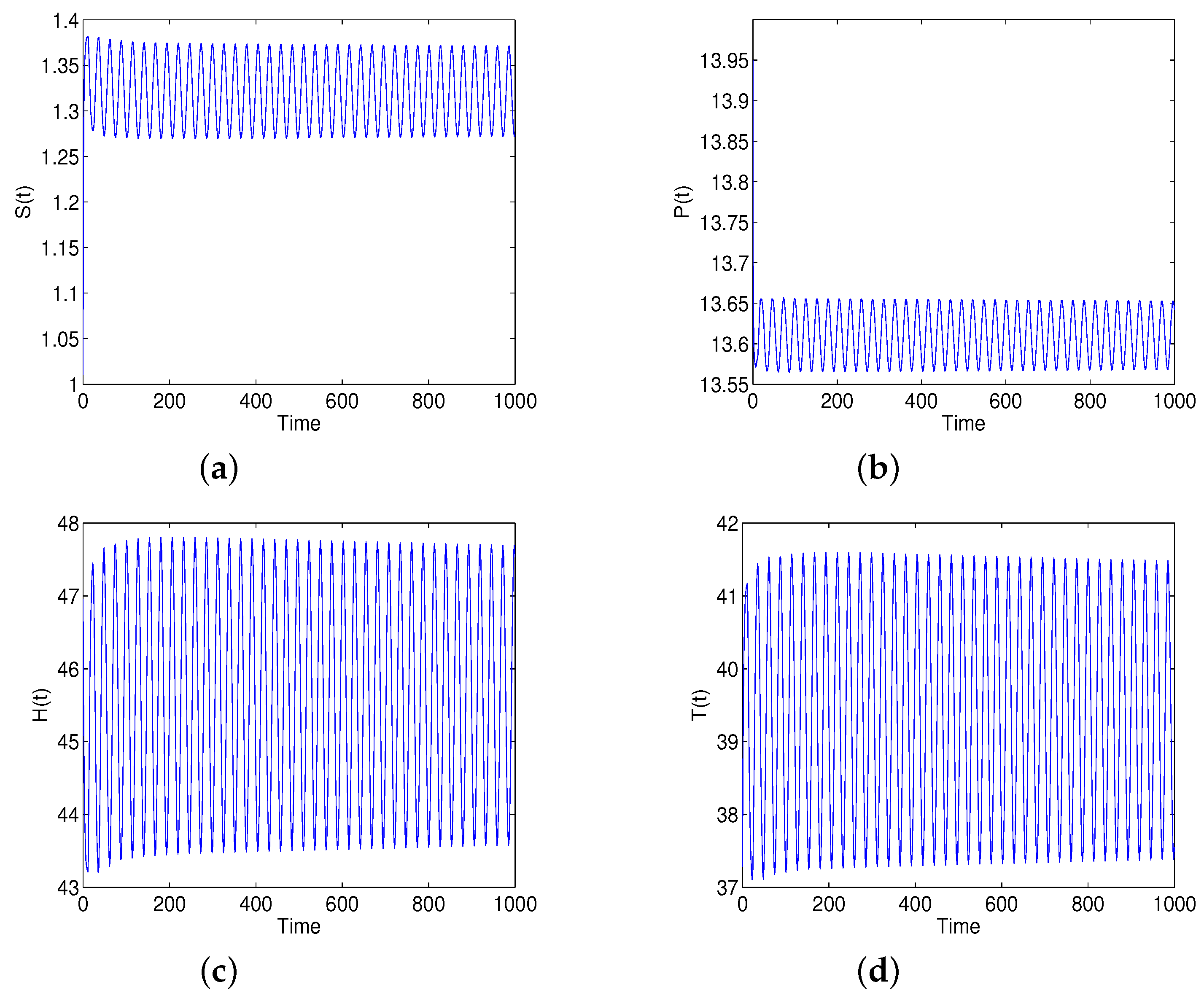
For the case when
and
, one has
and
. In line with Theorem 1,
is locally asymptotically stable in the interval
.
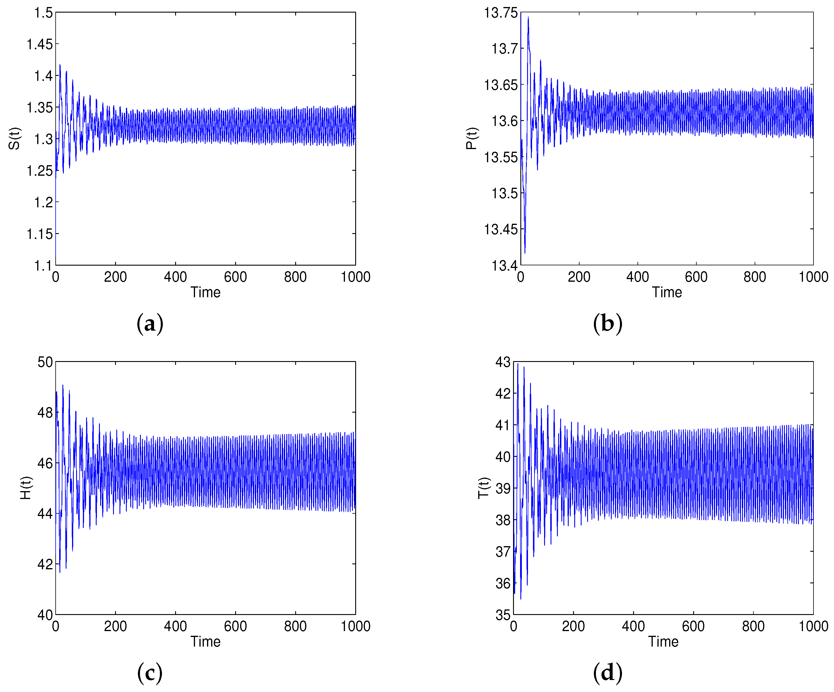
Figure 1 shows the local asymptotical stability of the model system (47). Whereas,
Figure 2 shows the exhibition of a Hopf bifurcation at
.
For
and
, we have
and
based on some calculations. It can be observed that the model system (47) is locally asymptotically stable around based on some calculations. It can be observed that the model system (47) is locally asymptotically stable around
when
, which is depicted in
Figure 3. Nevertheless,
loses its stability and the model system (47) experiences a Hopf bifurcation as the value of
crossed
. The loss of stability dynamics of
for
is shown in
Figure 4.
For
and
and supposing
as a parameter, we obtain
and
through some computations. In such a case, the model system (47) is locally asymptotically stable when
but as
passes through
the model system (47) exhibits a Hopf bifurcation and the model system (47) loses stability. This property is depicted in
Figure 5 and
Figure 6 for
and
, respectively.
For
and
and supposing
as a parameter, we get
and
. The model system (47) is locally asymptotically stable for
and unstable for
. Stability and instability behavior of the model system (47) is presented in
Figure 7 and
Figure 8 for different values of
, respectively.
In addition, for and , we obtain and . Thus, we have , and . Based on the Theorem 5, we can see that the Hopf bifurcation at is supercritical; the bifurcating periodic solutions showing around are stable, and the bifurcating periodic solutions showing around are decreasing.


