1. Introduction
A brain–computer interface (BCI) provides an alternate link to the external world for a subject using brain signals [
1]. BCIs are especially useful for patients with impaired peripheral nerve or muscle functions to rebuild connection to the real world. For healthy people, BCIs can also provide a new control dimension, such as in games [
2].
Motor imagery (MI)-based BCIs are the main type of BCIs. MI-BCIs are driven by neural signals modulated by users’ voluntary movement imagination [
3]. MI-related characteristic changes occur in some regions of the brain, especially the primary sensorimotor area and supplementary motor area [
4]. These changes can be acquired through electroencephalograms (EEG). MI information in EEG can be captured through spatial filtering methods, such as common spatial pattern (CSP) [
5], and then classified by machine learning methods to identify the intention of BCI users.
In machine learning theory, the data distributions of the training and test sets are supposed to be similar [
6]. However, the non-stationarity of EEG leads to high variability across different recording sessions [
7], which becomes a major obstacle to the accurate classification of EEG patterns. Studies indicate that the non-stationarity nature of EEG is induced by several factors, including physiological artifacts, state of subjects, and instrumental artifacts over different sessions [
8]. To overcome this problem, transfer learning methods are proposed [
9,
10].
Transfer learning is widely investigated, including inductive transfer learning, transductive transfer learning, and unsupervised transfer learning [
11]. Specifically, inductive transfer learning is employed when the source and target tasks are different [
12]. In this case, the source data is not labeled. Unsupervised transfer learning deals with the situation where the source and target tasks are similar, but labels of all data are unavailable. Transductive transfer learning deals with the situation in which the source data are labeled while the target data are unlabeled. Domain adaptation is related to transductive transfer learning, which is implemented based on the assumption that the source and target data are generated in the same task and distributed in different domains. Moreover, pre-trained models (with [
13] or without [
14] fine-tuning) are also introduced to search the shared feature patterns and reduce calibration with deep learning methods. Domain adaptation methods can easily learn the knowledge of labeled data in the source domain and transfer the knowledge to the target domain.
Recently, domain adaptation became a widely investigated approach to bridge the gap between the training set (i.e., the source domain) and the test set (i.e., the target domain) in the BCI field [
15]. This technology aims at reducing the distribution shifting of the source and target domains. [
16]. However, two issues arise, namely, the measurement of the discrepancy of different domains and the reduction of the discrepancy. Different measurement criteria are used to estimate the discrepancy between the source and target domains. Arithmetic mean, covariance, and correlation coefficients of data in source and target domains are frequently used as the statistical characteristics of distributions when performing alignment in data space [
17,
18,
19,
20]. Zheng et al. proposed a model based on transfer learning in which the mean and variance were used as the statistical characteristics shared across sessions [
21]. Liang et al. aligned the tangent space mapping features according to the Riemannian center to handle the instability of channel covariance across sessions [
22]. Azab et al. evaluated the distance between EEG data in the two domains using Kullback–Leibler (KL) divergence [
12]. The spatial projection filters were then weighted by the divergence. In the regularized common spatial pattern (RCSP) method, optimization was used to obtain the spatial project matrix of the source and target EEG data simultaneously to minimize the distance between them [
23]. The similarities between the two domains were also evaluated using other distance metrics, such as the Frobenius norm, Bhattacharyya distance, and cosine distance [
24,
25,
26].
The single statistical characteristic that was investigated in previous studies may not estimate the data distribution properly, which may further influence the discrepancy minimization between the source and target domains. Furthermore, the estimation of the data distribution of the unlabeled data in the target domain is difficult. Mean and covariance are two important characteristics of data distribution. Due to the non-stationarity of EEG, they may be quite different in the source and target domains of BCI [
7]. For this reason, a classifier trained with the source data may not perform well on the target data. Generally, the performance of classification depends on the similarity of the two domains [
27]. Thus, transferring the data distribution of the source domain to the target domain may result in a more accurate classification.
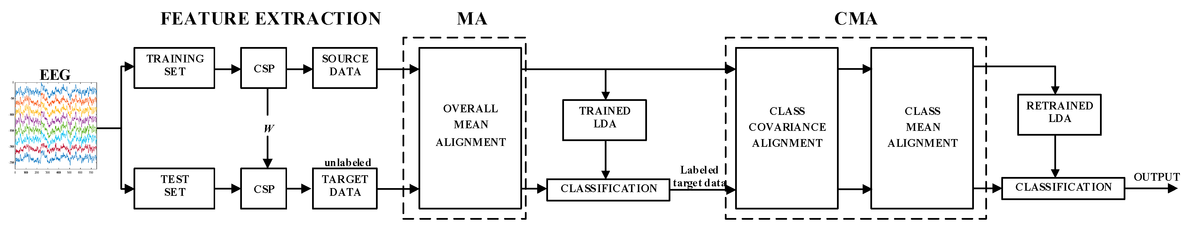
To minimize the discrepancy between the source and target domains, an unsupervised method based on the alignment in Euclidean space is proposed in this paper. There are two major contributions. First, the discrepancy of distribution between the two domains is removed completely using this method. Second, the mean alignment and covariance alignment for each class can be realized simultaneously. In this method, mean and covariance are used to represent the center and dispersion of the data distribution in the two domains. The alignment contains two stages, namely the mean alignment (MA) and the per-class covariance and mean alignment (CMA). In the MA stage, considering that the mean and covariance of each class in the source and target domains may vary enormously and the data in the target domain remain unlabeled, the mean of the source data is aligned with the data mean in the target domain. The data in the target domain remain unchanged. After MA, a linear discriminant analysis (LDA) classifier is trained using the source data. Then, the LDA classifier is used to classify the target data. According to the predicted labels estimated by the classifier, the per-class basis covariance (CA) of the target data is calculated. The covariance of the source data is then transformed to be the same as the covariance of target data for each class. After the covariance alignment, per-class basis MA is conducted again.
The remainder of this paper includes four sections.
Section 2 introduces the details of the proposed method. In
Section 3, the experimental datasets are introduced, and the experimental results are given.
Section 4 presents the discussions, and
Section 5 presents the conclusion.
3. Results
Two datasets were used to evaluate the proposed method. The first dataset (dataset 1) is the BCI competition III dataset IVa [
33]. Five subjects were guided to make the left hand, right hand, and right foot MI during EEG recording. For each subject, 280 EEG trials were obtained. The BCI competition IV dataset IIa [
34] was used as the second dataset (dataset 2). Nine subjects participated in MI EEG recording. The recorded EEG data correspond to four classes of MIs (i.e., left hand, right hand, both feet, and tongue MIs). There are two sessions in dataset 2. Each session is comprised of 144 trials. The two sessions were recorded on two days. In this study, only two-class MI data (left hand vs. right hand) for each dataset were selected for classification. The EEG data were preprocessed by a band-pass filter (8 Hz to 30 Hz). In addition, classification accuracy was calculated based on five-fold cross validation.
The proposed CSP-MA-CMA method was compared with three competing methods, namely CSP, CSP-MA, and CSP-MA-CA. In all four methods, CSP and LDA were used for MI feature extraction and classification, respectively. In the CSP-MA method, after feature extraction by CSP, overall mean alignment was conducted. As for CSP-MA-CA, overall mean alignment and per-class covariance alignment were performed sequentially after CSP feature extraction. All the methods were tested with MATLAB 2016b on a PC with a 3.5 GHz processor and 8.0 GB RAM.
Table 1 and
Table 2 show the classification accuracies of the four methods on the two datasets. As shown in
Table 1, compared with CSP, CSP-MA and CSP-MA-CMA improved the average accuracy by 1.3% and 2.3%, respectively, on dataset 1. As shown in
Table 2, CSP-MA and CSP-MA-CMA improved the average accuracy by 3.1% and 3.3%, respectively, on dataset 2 compared to CSP. However, the classification performances of CSP-MA-CA on both datasets only reached the chance level. Moreover, an additional public EEG dataset with two-class data (i.e., left hand and right hand MIs) from 52 subjects is used to evaluate the proposed method. For each subject, 200 trials were recorded during the experiment. More information on this dataset is provided in [
35]. The average accuracies of CSP and CSP-MA-CMA (the proposed method) are 56.32% and 58.46%, respectively.
To test the statistically significant differences between different alignment methods, a paired t-test was used. There were no significant differences in classification accuracy between CSP and CSP-MA on dataset 1 (p > 0.1) and dataset 2 (p = 0.09), although CSP-MA increased the average accuracy. The performance of CSP-MA-CMA increased significantly compared with CSP on dataset 1 (p = 0.03) and dataset 2 (p = 0.04), as well as the additional dataset (p = 0.02).
Datasets 1 and 2 are commonly used for MI EEG classification, whereas only a few methods not related to transfer learning are evaluated based on the above mentioned MI dataset from 52 subjects. Thus, the comparison between the proposed method and the methods in some previous studies was conducted only on datasets 1 and 2. As shown in
Table 3 and
Table 4, the best average accuracy was achieved by the proposed method.
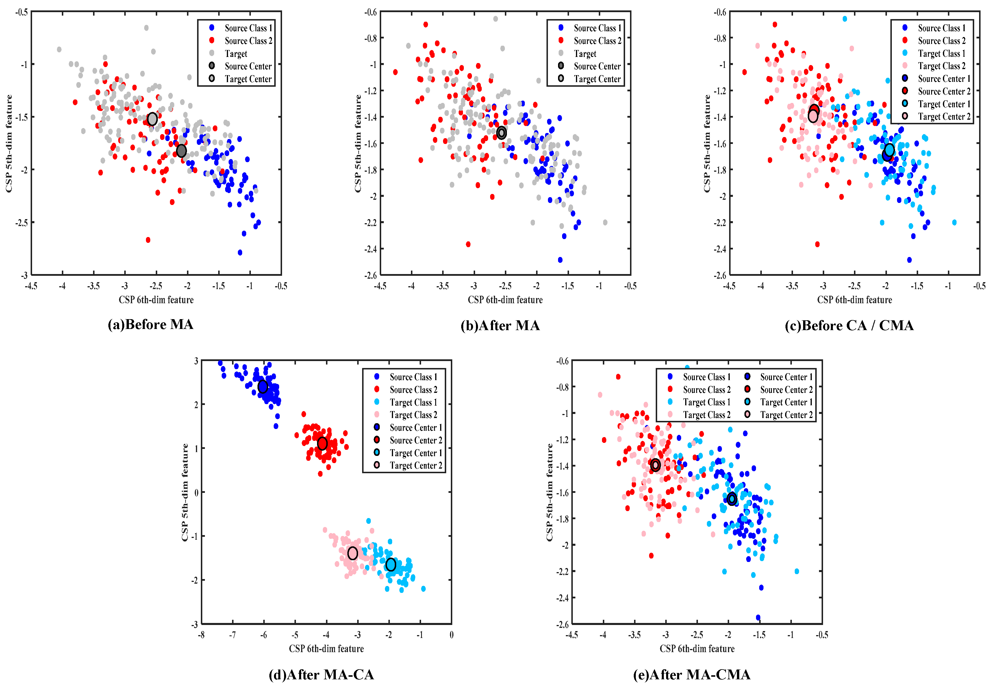
The visualization of data distribution during the alignment process clearly shows how the data distribution was modified by the proposed CSP-MA-CMA method. The distribution of original features before and after different kinds of alignments in the two domains for subject 3 in dataset 2 is shown in
Figure 2. To facilitate visualization, the last two dimensions of the EEG features, namely the sixth and fifth dimensions, were used for data distribution representation. The distribution before MA is shown in
Figure 2a. The dots in dark blue are the samples of class 1, and those in dark red are the samples of class 2 in the source domain. The grey dots represent the unlabeled samples in the target domain. Two larger dots in dark grey and light grey show the overall centers in the two domains, respectively. They are different from each other before MA.
The data distribution after MA is shown in
Figure 2b. The data in the source domain were aligned by MA to have the same center as the data in the target domain. The classifier was trained using the mean aligned data in the source domain and then used for data classification in the target domain. As shown in
Figure 2c, the target data were divided into different classes by the pre-trained classifier, which are represented as class 1 in light blue and class 2 in light red, respectively. For each class, the mean and covariance of the data in the two domains were different. The data distribution after MA-CA and MA-CMA is shown in
Figure 2d,e, respectively. In
Figure 2d, although the per-class covariance in the two domains was forced to be equal after MA-CA, the difference between the means of the data in the two domains increased, which may be the reason for the low classification accuracy of the CSP-MA-CA method shown in
Table 1 and
Table 2. Therefore, it is necessary to align the means of each class as the last step, which does not change the aligned class covariance in the two domains.
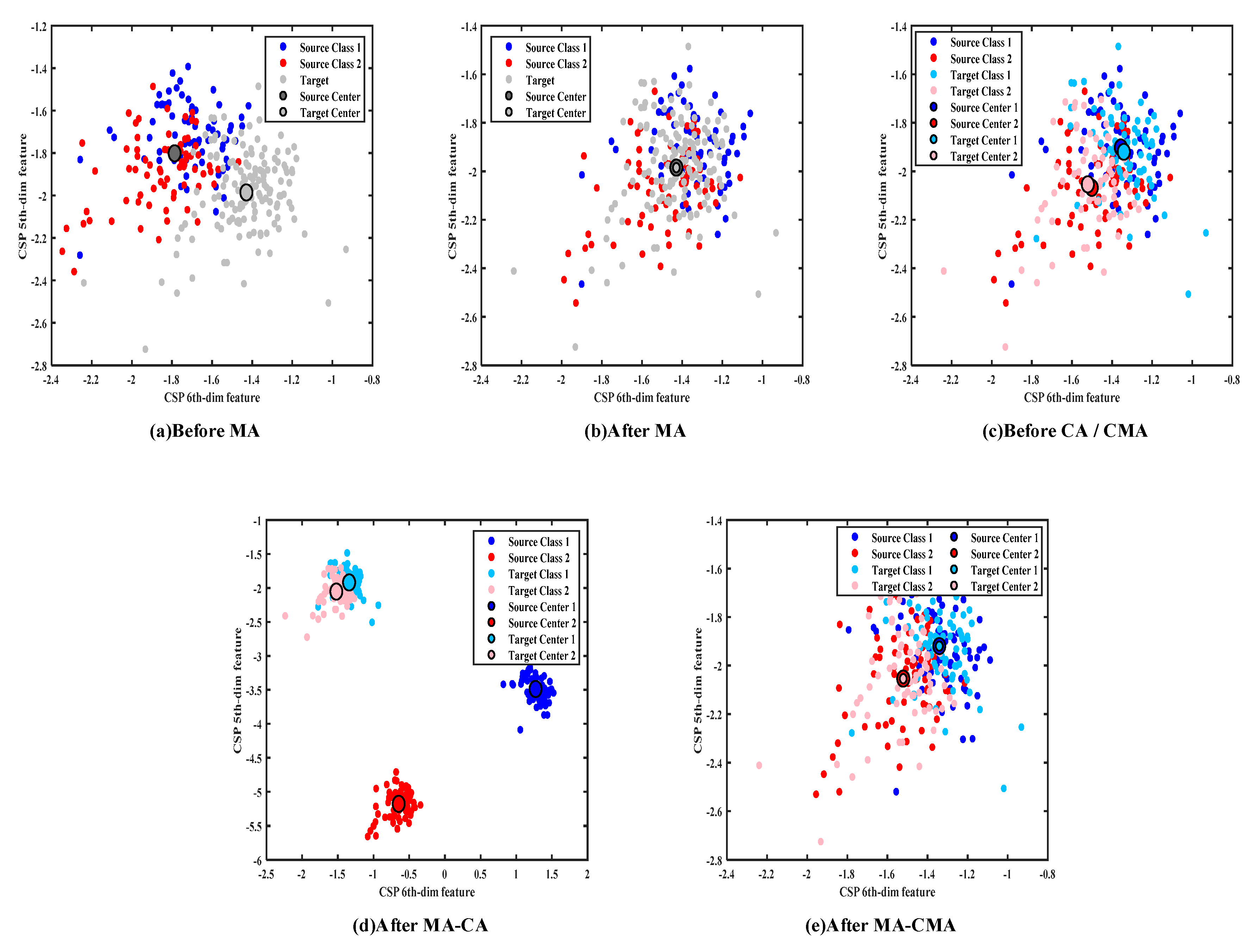
The data distribution of subject 5 in dataset 2 is shown in
Figure 3. Similar results after each alignment step can be observed.


