Three-Echelon Supply Chain Management with Deteriorated Products under the Effect of Inflation

Abstract

A business can be properly managed globally when it is under a supply chain. When it is a global supply chain, inflation has a huge effect on supply chain profit. Another important factor is the deterioration of products. Products can deteriorate during storage or transportation, which badly affects each supply chain player. This study develops a three-echelon supply chain model through which products can be delivered to customers easily. In this model, one producer and multiple buyers are considered, and each buyer has a separate group in which multiple suppliers have been taken. Inflation is also added to the model for inflationary fluctuations. To understand this model in real life, a numerical example is discussed and the total profit from the supply chain is extracted. Sensitivity analysis is also shown at the end of the model to find out the effect on the model due to changes in some parameters that affect this model highly. After developing this model, it was found that if the inflation rate falls, then the total profit will increase continuously. On the contrary, if the inflation rate increases, then, in this situation, the total profit will decrease continuously. At present, vaccine makers’ total profit can support the economy of any country, and in this model, the inflation rate decreases as profit increases.

1. Introduction

With the competition that has arisen in every trade at the present time, one thing is certain—it becomes more important for every business to reach its customers in maximum quantity at reasonable prices and at the time required by the customer. The three-echelon supply chain (TESC) system has played an important role in all these things because TESC management acts like an organization. It is the responsibility of all the members working in this organization to fulfill all the needs of the customer and to make every step of the supply chain system highly profitable from this trade. During the period of COVID-19, the worldwide lockdown affected the economies of many countries in such a way that they will feel the COVID effects for many years to come due to the work-from-home mandates in the lockdown and many other reasons. Many authors have discussed the impact of inventory management on economic conditions. Asghar et al. [1] developed a smart automatic inventory model (IM) based on an economic production policy that covers high-technology items such as mobile phones, computers, electronic devices, etc. Mallick et al. [2] formulated an IM with permissible delay in payment and time-dependent demand. Supply chain management acts like an organization, and it is the responsibility of all the members to fulfill all the needs of the customers and to make every step of the supply chain system highly profitable. Mashud et al. [3] investigated a sustainable IM under controllable emission for imperfect products. Bachar et al. [4] developed a sustainable IM with a flexible production system under carbon reduction technology. Sarkar et al. [5] formulated a sustainable production IM with a single type of item, where all the items are transported to the consumer by only one transportation mode with a shortage under the reduction of carbon emissions.

The contribution of this study can be illustrated as follows:

• A three-echelon supply chain model is considered with single-producer and multi-buyers, and each buyer deals with a separate group of multi-sellers. Each supply chain player has an individual cycle time.
• Products deteriorate at each supply chain player with different deterioration rates. The aim of each supply chain player is to sell the product to the customer at the right time and in good quality.
• Inflation has a very important effect on any global business. The product’s price and other costs vary with inflation. In this study, the effect of inflation on supply chain management is discussed elaborately.

The next part of the manuscript is arranged as follows: Section 2 describes the literature review, which shows the research gap with the proposed study. Assumptions, notation, and mathematical modeling are explained in Section 3. Section 4 represents the solution methodology, where the algorithm, numerical examples, and comparison with existing literature are included. Sensitivity analysis and managerial insights are included in Section 5. At the end, conclusions are discussed in Section 6.

2. Literature Review

In this part, a literature review of supply chain management (SCM), inflation, and deteriorating items are discussed, which is the base of this model.

2.1. Classical IM with Deteriorating Items

Inventory is a form of physical resource that keeps any business running efficiently. There are many types of products in the market that have their own period of survival or safe use. After this period, these products are seen to decline; these products are called deteriorating items. Many products in the market can be returned in the event of damage. However, many products are not returned after spoilage, such as dairy products and medicines. Many authors have developed several IMs for deteriorating products. Rau et al. [6] formulated the multi-echelon inventory model (MEIM) for bad goods. Rani et al. [7] formulated an IM by developing green SCM for deteriorating products. They took demand as a function of the credit period. Shaikh et al. [8] discussed an IM for deteriorating items under preservation technology and shortage. They used demand as a ramp type and policy of trade credit. Gupta et al. [9] introduced an IM with the help of storage problems and partial backlogging for deteriorating items and trade credit policy. Padiyar et al. [10] developed an IM with price-dependent demand for deteriorating items under an imprecise environment. Hasan [11] developed a production inventory model for deteriorating goods under COVID-19 disruption risks. Kumar et al. [12] formulated an inventory system for deteriorating products with a demand-dependent production rate under permissible delay payments.

2.2. Inventory Management in Supply Chain

The supply chain inventory model (SCIM) generally considers different sub-systems. Recently, due to changes in transmission and information technologies, the consolidations of these functions have appeared normal. Most researchers have discussed the inventory model with the help of producers, retailers, and buyers. Chou [13] developed an IM for deteriorating items. Rani and Kishan [14] described an MEIM for deteriorating items. Demand is variable in the model. Habib et al. [15] developed an SCIM with imperfect biodiesel production under a flexible approach. Jaggi et al. [16] developed an IM for deteriorating items in a fuzzy sense using time-varying demand. Barman et al. [17] formulated an integrated IM with fuzzy variables, variable holding cost, and a three-parameter Weibull deterioration rate. Rana et al. [18] developed an MEIM with two warehouses, imperfect production, and inflation. In that study, the demand was variable. Sarkar et al. [19] formulated an SCIM for damaged items and considered demand and production as fuzzy variables with preservation technology (PT) and shortages. Maihami et al. [20] discussed a TESCM with deteriorating items under a probabilistic environment. Sarkar et al. [21] introduced a joint IM for an online-to-offline closed-loop supply chain. Jiang et al. [22] formulated a sustainable SCIM under carbon footprint consideration. Sebatjane and Adetunji [23] developed an MEIM with price-dependent demand for an economically growing quantity model. Sana [24] introduced a structural model on MEIM. Lu et al. [25] developed a multistage sustainable production model with carbon reduction and a Stackelberg game. In that model, demand depended on price. Jauhari et al. [26] discussed a closed-loop SCIM under carbon emission. Pandiyar et al. [27] developed an inventory model for deteriorating items withprice-dependent consumption and shortages under a fuzzy environment. Karimi and Sadjadi [28] formulated an optimization technique for a multi-item inventory model for deteriorating goods under capacity constraints utilizing the approach of dynamic programming.

2.3. Inflation in Supply Chain Management

Inflation is measured as an annual percentage increase. Tiwari et al. [29] discussed an IM with quadratic demand for deteriorating goods with inflation and trade credits. Mukherjee et al. [30] discussed a lot size model for deteriorating items studied under inflation. Mahapatra et al. [31] investigated a model with inflation within a finite planning horizon. The subject of the paper was to find out the optimal replenishment schedule for an IM; demand was time-dependent, and a finite time planning horizon was assumed. Palanivel and Uthayakumar [32] proposed a two-warehouse IM for deteriorating items with a credit period, inflation, and partial backlogging. Singh et al. [33] formulated a two-warehouse IM for damaged items with variable demand and partial backlogging under inflation. Agarwal et al. [34] formulated an IM for deteriorating goods with an exponential demand rate under a partially backlogged shortage of items with inflation. Singh and Rana [35] formulated a model with inflation, lost sales, multi-variable demand, and variable holding costs. Alamri et al. [36] developed an EOQ model with carbon emissions and inflation for deteriorating imperfect quality items under the learning effect. Alfares and Attia [37] studied a vendor–buyer model with errors in a quality inspection under the effect of volume agility, whereas Jaggi et al. [38] proposed an optimal order policy for deteriorating items with inflation. Additionally, Padiyar et al. [39] developed an inventory model with a limited storage problem for perishable items in an uncertain environment.

2.4. Deterioration during Transportation

Transporting perishable items requires precise control and security operations due to their short rack life or specific capacity circumstances Aghighi et al. [40] developed a location-routing-inventory problem (LRIP) for perishable items under a stochastic demand consideration. They used the concept of price reneging for their model; however, instead of the supply chain, they considered the inventory problem. In a similar direction, a supply chain model for the healthcare system was formulated by Goli et al. [41]. Goli et al. [41] developed a possibilistic programming model for organ transplantation center location management. A sustainable supply chain under a fuzzy bi-level decision support system for a perishable product was developed by Trikolaee and Aydin [42]. Trikolaee and Aydin [42] formulated the model for multi-products, and a transportation network configuration was also presented in their study. A two-echelon supply chain under a location–allocation–routing transportation strategy for a sustainable product was developed by Trikolaee et al. [43]. They used the Grey Wolf Optimization (GWO) and Particle Swarm Optimization (PSO) techniques for their study and proved that the GWO technique provided a better result compared to PSO. Similarly, Alinezhad et al. [44] proposed a closed-loop sustainable supply chain system for food industries. Alinezhad et al. [44] used bi-objective fuzzy logic to optimize the total profit of the system under the consideration of carbon footprints.

In this study, we have mentioned all factors in a model to better match the problem with realistic situations. This model is a co-partnership of buyer, supplier, and vendor. Here, an effort is accomplished to formulate a TESCM for deteriorating items under inflation. Whenever the whole world is affected by a terrible disease such as COVID, it is suddenly seen that the entire economy is affected, and all the countries are very worried about their economy. Then, every country will want to strengthen its economy by manufacturing and supplying items to foreign countries as soon as possible for the various types of terrible diseases; with this thinking in mind, this model was developed for maximum benefit to the supply chain and the analysis was by manufacturing the different types of inventory and delivering it to the last member of the supply chain. The research gap with the existing literature is explained in

Table 1. Author(s) contribution table.

Authors	Model Type	Transportation Cost	Deterioration	Inflation
Karimi and Sadjadi [28]	Inventory	NC	Considered	NC
Alamri et al. [36]	Inventory	NC	Considered	Considered
Sarkar et al. [45]	SCM	Variable	NC	NC
Padiyar et al. [46]	SCM	NC	Considered	Considered
Mahapatra et al. [47]	Inventory	NC	Considered	Considered
Fallah and Nozari [48]	SCM	Considered	NC	NC
Sundararajan et al. [49]	Inventory	NC	Considered	Considered
Gupta et al. [50]	SCM	Variable	NC	NC
Khan et al. [51]	Inventory	NC	Considered	NC
Dey et al. [52]	SCM	Variable	NC	NC
Chakraborty et al. [53]	Inventory	Considered	Considered	Considered
Khan et al. [54]	Inventory	NC	Considered	NC
Duary et al. [55]	Inventory	Considered	Considered	NC
Shah and Naik [56]	Inventory	NC	Considered	NC
This study	SCM	Fixed and Variable	Considered	Considered

NC: Not considered for this study.

.

3. Mathematical Model

3.1. Assumptions

• A supply chain has been used to develop this model in which three members have been kept in the main roles, which are producer, supplier, and buyer, in which the producer is a company that manufactures the inventory and delivers it to each buyer; after that, the buyer delivers the items to the suppliers, which may vary in number for each buyer.
• Some inventory may become imperfect while being transported. Additionally, the total rate of this imperfect quality inventory is considered as the deteriorating items.

3.2. Notation

• $P$ production rate for the producer
• $D$ demand rate for the producer
• ${\theta }_1$ deterioration rate for the producer
• ${\psi }_{\alpha }$ selling price for the producer for the αth buyers $\alpha$= 1, 2, 3 … m
• $A_c$ setup cost of producer per setup
• $h_p$ holding cost for the producer
• $d_p$ deterioration cost for the producer
• $T_p$ fixed transport cost for the producer
• $t_{\alpha }$ variable transportation cost in transporting inventory from the producer to the αth buyer
• $L_{\alpha }$ demand rate for the αth buyer
• ${\theta }_2$ deteriorating rate for each buyer
• $J$ total number of shipments to the buyer from the producer
• $R$ total number of shipments to the supplier from the buyer
• ${\varphi }_{\alpha {\beta }_{\alpha }}$ selling price for the αth buyer to the suppliers
• $h_{\alpha }$ holding cost for the αth buyer
• $d_{\alpha }$ deterioration cost of the αth buyer
• $A_{\alpha }$ ordering cost of the αth buyer
• $T_{B\alpha }$ fixed transportation cost charged in carrying inventory from the αth buyer to the supplier.
• ${\gamma }_{\alpha {\beta }_{\alpha }}$ variable transportation cost charged in carrying inventory from the αth buyer to the supplier’s group
• $D_{\alpha {\beta }_{\alpha }}$ demand rate of the αth group of the suppliers
• ${\theta }_3$ deteriorating rate for each supplier.
• $h_{\alpha {\beta }_{\alpha }}$ supplier’s holding cost of the αth group
• $d_{\alpha {\beta }_{\alpha }}$ supplier’s deterioration cost of the αth group
• $A_{\alpha {\beta }_{\alpha }}$ supplier’s ordering cost of the αth group
• ${\sigma }_{\alpha {\beta }_{\alpha }}$ selling price for the αth group of suppliers

3.3. Model Formulation

The main objective of developing this model was to transport any product from the production house to the end consumer on time and safely. Therefore, a multi-echelon supply chain model has been created. It is important to manufacture different types of products and transport them at the right time to all the customers, and they should be of good quality. The supply chain model plays a very important role in this principle. This study has formulated a supply chain model at three levels, in which the company plays the role of the producer and other supply chain members are the buyers and the suppliers, which are divided into different groups. Here, each buyer orders the inventory according to their needs.

3.3.1. Model for Producer

In this proposed IM, one producer is considered. Here, the producer produces the inventory according to the needs of each buyer. The entire inventory cycle is classified into two parts, giving time intervals [0, $T_1]$ and [$T_1, T]$. In the time interval [0, $T_1],$ there is a mixed impact of production, deterioration, and demand on the quantity. In the time interval [$T_1, T],$ the inventory is only affected by the demand and deterioration. The following equations can represent the producer’s IM:

$$\frac{d{Q}_{P1}\left(t\right)}{dt}=P-D-{\theta }_1{Q}_{P1}\left(t\right), 0\le t\le T_1$$

(1)

$$\frac{d{Q}_{P2}\left(t\right)}{dt}=-D-{\theta }_1{Q}_{P2}\left(t\right), T_1\le t\le T$$

(2)

With the help of boundary conditions $Q_{P1}\left(0\right)$ = 0, $Q_{P2}$(T) = 0, the solutions of Equations (1) and (2) are

$$Q_{P1}\left(t\right)=\frac{\left(P-D\right)}{{\theta }_1}\left[1-e^{-{\theta }_{1}t}\right]$$

(3)

$$Q_{P2}\left(t\right)=\frac{D}{{\theta }_1}\left[e^{{\theta }_1\left(T-t\right)}-1\right]$$

(4)

Lemma 1.

Demand rate (D), production rate (P), cycle time length (T), and production time ($T_1)$must satisfy the relation

$$T_1=\frac{1}{{\theta }_1}log\left[\frac{D}{P}{e}^{{\theta }_{1}T}+1-\frac{D}{P}\right]$$

Proof. 

From Equation (3), we have

$$Q_{P1}\left(T_1\right) = \frac{\left(P-D\right)}{{\theta }_1}\left[1-e^{-{\theta }_1{T}_1}\right]$$

and from Equation (4), we have

$$Q_{P2}\left(T_1\right) = \frac{D}{{\theta }_1}\left[e^{{\theta }_1\left(T-T_1\right)}-1\right]$$

At point t =$T_1$ both $Q_{P1}$($T_1$) and $Q_{P2}$($T_1$) are equal, so

$$\frac{\left(P-D\right)}{{\theta }_1}\left[1-e^{-{\theta }_1{T}_1}\right]=\frac{D}{{\theta }_1}\left[e^{{\theta }_1\left(T-T_1\right)}-1\right]$$

$$P=e^{-{\theta }_1{T}_1}\left[D{e}^{{\theta }_{1}T}-D+P\right]$$

$$T_1=\frac{1}{{\theta }_1}log\left[\frac{D}{P}{e}^{{\theta }_{1}T}+1-\frac{D}{P}\right]$$

□

To calculate the producer’s total profit, one needs to calculate the following factors:

Sales Revenue

Sales revenue is the income created by offering and conveying items or administrations to buyers. The total sales revenue for the producer is:

$$SR{C}_P={{\displaystyle \sum }}_{\alpha =1}^m{\psi }_{\alpha }\left(Q_{B\alpha }\right)\left(\frac{1-e^{-jr{T}_2}}{1-e^{-r{T}_2}}\right)$$

(5)

Setup cost

To start any production system, the initial setup is essential. The cost is needed for each setup of production. If $A_c$ is the setup cost per setup, the setup cost of the producer per cycle can be written as

$$S_c={{\displaystyle \int }}_0^T{A}_c{e}^{-rt}dt$$

(6)

Holding cost

Holding fetched is included in the cautious capacity and support of stock, counting equipment hardware, and fabric dealing with equipment and IT computer program applications. Hence, the holding cost for the maker is:

$$H_P=h_p\left[{{\displaystyle \int }}_0^{T_1}{Q}_{P1i}\left(t\right)e^{-rt}dt+{{\displaystyle \int }}_{T_1}^T{Q}_{P2i}\left(t\right)e^{-rt}dt\right]$$

$$H_P=h_p\left[\begin{array}{c}\left(\frac{P-D}{{\theta }_1}\right)\left\{\left(\frac{1-e^{-r{T}_1}}{r}\right)+\left(\frac{e^{-\left({\theta }_1+r\right)T_1}-1}{{\theta }_1+r}\right)\right\}+\\ \frac{D}{{\theta }_1}\left\{e^{{\theta }_{1}T}\left(\frac{e^{-\left({\theta }_1+r\right)T_1}-e^{-\left({\theta }_1+r\right)T}}{{\theta }_1+r}\right)+\left(\frac{e^{-rT}-e^{-r{T}_1}}{r}\right)\right\}\end{array}\right]$$

(7)

Deterioration cost

Deterioration cost is included due to the weakening of things that end up being worthless. Therefore, one can calculate the deterioration fetched for the maker as follows:

$$D_P={\theta }_1{d}_p\left[{{\displaystyle \int }}_0^{T_1}{Q}_{P1i}\left(t\right)e^{-rt}dt+{{\displaystyle \int }}_{T_1}^T{Q}_{P2i}\left(t\right)e^{-rt}dt\right]$$

$$D_P={\theta }_1{d}_p\left[\begin{array}{c}\left(\frac{P-D}{{\theta }_1}\right)\left\{\left(\frac{1-e^{-r{T}_1}}{r}\right)+\left(\frac{e^{-\left({\theta }_1+r\right)T_1}-1}{{\theta }_1+r}\right)\right\}+\\ \frac{D}{{\theta }_1}\left\{e^{{\theta }_{1}T}\left(\frac{e^{-\left({\theta }_1+r\right)T_1}-e^{-\left({\theta }_1+r\right)T}}{{\theta }_1+r}\right)+\left(\frac{e^{-rT}-e^{-r{T}_1}}{r}\right)\right\}\end{array}\right]$$

(8)

Transportation cost

Transportation is one of the foremost crucial costs for a supply chain, and it cannot continuously be treated as settled. In this study, transportation cost is separated into two categories: one is settled, and the other is variable. Variable transportation fetched depends on the real development of traffic, which incorporates the fuel cost and cost of upkeep of the vehicle. It is totally subordinate to the conveyance of things, amount, and area. Fixed transportation costs incorporate the month-to-month installment of the vehicle, vehicle protection, driver’s compensation, and authoritative and administrative costs. Therefore, the transportation cost for the maker can be mathematically presented as:

$$TP{C}_P=T_P+{{\displaystyle \sum }}_{\alpha =1}^m\left(Q_{B\alpha }\right)t_{\alpha }\left(\frac{1-e^{-rj{T}_2}}{1-e^{-r{T}_2}}\right)$$

(9)

The total profit cost for the producer depends on all the above costs. The total profit cost for the producer is:

$${\prod }_P=\frac{1}{T}\left[SR{C}_P-S_c-H_P-D_P-TP{C}_P\right]$$

(10)

Lemma 2.

When the cycle length T is fixed, then the total profit function${\prod }_P\left(T,T_1\right)$is concave w.r.t the time length$T_1$if

$$T > \frac{1}{{\theta }_1}log\left[\frac{rP}{D\left({\theta }_1+r\right)}{e}^{{\theta }_1{T}_1}-\frac{P}{D}+1\right]$$

Proof. 

Using Equations (1)–(10);

All first- and second-order partial derivatives of the function ${\prod }_P\left(T,T_1\right)$ with respect to $T_1$ are

$$\frac{\partial {\prod }_p\left(T_1,T\right)}{\partial T_1}=-\frac{1}{T}\left[\left(h_p+{\theta }_1{d}_p\right)\left[\begin{array}{c}\left(\frac{P-D}{{\theta }_1}\right)\left[e^{-r{T}_1}-e^{-\left({\theta }_1+r\right)T_1}\right]\\ +\frac{D}{{\theta }_1}\left[e^{{\theta }_{1}T}\left(-e^{-\left({\theta }_1+r\right)T_1}\right)+e^{-r{T}_1}\right]\end{array}\right]\right]$$

and

$$\frac{{\partial }^2{\prod }_p\left(T_1,T\right)}{\partial T_1{}^2}=-\frac{1}{T}\left[\left(h_p+{\theta }_1{d}_p\right)\left[\begin{array}{c}\left(\frac{P-D}{{\theta }_1}+\frac{D}{{\theta }_1}{e}^{{\theta }_{1}T}\right)\left[\left({\theta }_1+r\right)e^{-\left({\theta }_1+r\right)T_1}\right]\\ -\left[\frac{P-D}{{\theta }_1}+\frac{D}{{\theta }_1}\right]\left[r{e}^{-r{T}_1}\right]\end{array}\right]\right]$$

Let $\frac{{\partial }^2{\prod }_p\left(T_1,T\right)}{\partial T_1{}^2}<0,$ then $\left[\begin{array}{c}\left(\frac{P-D}{{\theta }_1}+\frac{D}{{\theta }_1}{e}^{{\theta }_{1}T}\right)\left[\left({\theta }_1+r\right)e^{-\left({\theta }_1+r\right)T_1}\right]\\ -\left[\frac{P-D}{{\theta }_1}+\frac{D}{{\theta }_1}\right]\left[r{e}^{-r{T}_1}\right]\end{array}\right]>0$

$$D{e}^{{\theta }_{1}T}>\frac{rP}{{\theta }_1+r}{e}^{{\theta }_1{T}_1}-P+D$$

$$T_1>\frac{1}{{\theta }_1}log\left[\frac{rP}{D\left({\theta }_1+r\right)}{e}^{{\theta }_1{T}_1}-\frac{P}{D}+1\right]$$

□

3.3.2. Model for Buyers

There are total m buyers, but each buyer has their own separate supply chain, under which there are different numbers of suppliers. At the beginning of the cycle $\alpha$th, the buyer receives $Q_{B\alpha }$ units of inventory from the multi-producers, which are transported in R shipments to their own group of suppliers.

The buyer’s inventory model can be defined by the equation

$$\frac{d{Q}_{B\alpha }\left(t\right)}{dt} =-L_{\alpha }-{\theta }_2{Q}_{B\alpha }\left(t\right), 0\le t\le T_2,$$

(11)

where $\alpha$ = 1, 2, 3 … m, and $Q_{B\alpha }\left(T_2\right)=0$.

The solution to Equation (11) is

$$Q_{B\alpha }\left(t\right)=\frac{L_{\alpha }}{{\theta }_2}\left(e^{{\theta }_2\left(T_2-t\right)}-1\right),$$

(12)

To calculate the buyer’s total profit, one needs to calculate the following factors;

Sales Revenue

Sales revenue is income created by offering and conveying items or administrations to suppliers. The total sales revenue for the buyer is

$$SR{C}_B=\left[{{\displaystyle \sum }}_{\alpha =1}^m{{\displaystyle \sum }}_{{\beta }_{\alpha }=1}^{{\lambda }_{\alpha }}{\phi }_{\alpha {\beta }_{\alpha }}{Q}_{S_{\alpha {\beta }_{\alpha }}}\right]\left[\frac{1-e^{-rjR{T}_3}}{1-e^{-r{T}_3}}\right]$$

(13)

$$s.t R{{\displaystyle \sum }}_{{\beta }_{\alpha }=1}^{{\lambda }_{\alpha }}{Q}_{S_{\alpha {\beta }_{\alpha }}}\le Q_{B\alpha }$$

where $\alpha$= 1, 2, 3 … m

Holding cost

Holding fetched is included in the cautious capacity and support of stock, counting equipment hardware, and fabric dealing with equipment and IT computer program applications. Hence, the holding cost for the buyer is:

$$H_B={{\displaystyle \sum }}_{\alpha =1}^m{{\displaystyle \sum }}_{\chi =1}^j{h}_{\alpha }\left[{{\displaystyle \int }}_{\left(\chi -1\right)T_2}^{\chi T_2}{Q}_{B\alpha }\left(t\right)e^{-rt}dt\right]$$

$$H_B={{\displaystyle \sum }}_{\alpha =1}^m{{\displaystyle \sum }}_{\chi =1}^j{h}_{\alpha }\frac{L_{\alpha }}{{\theta }_2}\left[\begin{array}{c}{e}^{{\theta }_2{T}_2}\left(\frac{e^{-\left({\theta }_2+r\right)\left(\chi -1\right)T_2}-e^{-\left({\theta }_2+r\right)\chi T_2}}{{\theta }_2+r}\right)\\ +\left(\frac{e^{-r\chi T_2}-e^{-r\left(\chi -1\right)T_2}}{r}\right)\end{array}\right]$$

(14)

Deterioration cost

Deterioration cost is included due to the weakening of things that end up being worthless. Therefore, one can calculate the deterioration fetched for the buyer as follows:

$$D_B={{\displaystyle \sum }}_{\alpha =1}^m{{\displaystyle \sum }}_{\chi =1}^j{d}_{\alpha }{\theta }_2\left[{{\displaystyle \int }}_{\left(\chi -1\right)T_2}^{\chi T_2}{Q}_{B\alpha }\left(t\right)e^{-rt}dt\right]$$

$$D_B={{\displaystyle \sum }}_{\alpha =1}^m{{\displaystyle \sum }}_{\chi =1}^j{d}_{\alpha }{L}_{\alpha }\left[\begin{array}{c}{e}^{{\theta }_2{T}_2}\left(\frac{e^{-\left({\theta }_2+r\right)\left(\chi -1\right)T_2}-e^{-\left({\theta }_2+r\right)\chi T_2}}{{\theta }_2+r}\right)\\ +\left(\frac{e^{-r\chi T_2}-e^{-r\left(\chi -1\right)T_2}}{r}\right)\end{array}\right]$$

(15)

Ordering cost

Ordering cost is the full fetched included in requesting the items, counting the cost of finding the maker, and assessing the stock. Therefore, the total cost for orders can be mathematically presented as follows:

$$O_B={{\displaystyle \sum }}_{\alpha =1}^m{A}_{\alpha }$$

(16)

Transportation cost

Transportation is one of the foremost crucial costs for supply chains, and it cannot continuously be treated as settled. In this study, transportation cost is separated into two categories: one is settled, and the other is variable. Variable transportation fetched depends on the real development of traffic, which incorporates the fuel cost and cost of upkeep of the vehicle. It is totally subordinate to the conveyance of things, amount, and area. Fixed transportation costs incorporate the month-to-month installment of the vehicle, vehicle protection, driver’s compensation, and authoritative and administrative costs. Therefore, the transportation cost for the buyer can be mathematically presented as:

$$TP{C}_B={{\displaystyle \sum }}_{\alpha =1}^m{T}_{B\alpha }+\left[{{\displaystyle \sum }}_{\alpha =1}^m{{\displaystyle \sum }}_{{\beta }_{\alpha }=1}^{{\lambda }_{\alpha }}{\gamma }_{\alpha {\beta }_{\alpha }}{Q}_{S_{\alpha {\beta }_{\alpha }}}\right]\left[\frac{1-e^{-rjR{T}_3}}{1-e^{-r{T}_3}}\right]$$

(17)

Total profit for the buyers depends on sales revenue, ordering cost, holding cost, deterioration cost, and transportation cost, so the total profit cost for the buyer is:

$${\prod }_B=\frac{1}{T}\left[SR{C}_B-H_B-D_B-O_B-TP{C}_B-SR{C}_P\right]$$

(18)

3.3.3. Model for Suppliers

There is a total of ${{\displaystyle \sum }}_{\alpha =1}^m{\lambda }_{\alpha }$ suppliers, which are classified into different groups. The $\alpha$th group has a total of ${\lambda }_{\alpha }$ suppliers, which are completely dependent on the $\alpha$th buyer and located in different locations. The first shipment of the buyer is delivered to the supplier at the beginning of the cycle, and the next shipment is received every $T_3$ time.

The supplier’s inventory system is represented by the following first-order linear differential equation.

$$\frac{d{Q}_{S_{\alpha {\beta }_{\alpha }}}\left(t\right)}{dt} =-D_{\alpha {\beta }_{\alpha }}-{\theta }_3{Q}_{S_{\alpha {\beta }_{\alpha }}}\left(t\right), 0\le t\le T_3$$

(19)

$$A=1,2,3 \dots m \mathrm{and} {\beta }_{\alpha } =1,2,3\dots {\lambda }_{\alpha }$$

With $Q_{S_{\alpha {\beta }_{\alpha }}}\left(T_3\right)$ = 0, the solution of Equation (18) is

$$Q_{S_{\alpha {\beta }_{\alpha }}}\left(t\right)=\frac{D_{\alpha {\beta }_{\alpha }}}{{\theta }_3}\left(e^{{\theta }_3\left(T_3-t\right)}-1\right)$$

(20)

To calculate the supplier’s total profit, one needs to calculate the following factors;

Sales Revenue

Sales revenue is income created by offering and conveying items or administrations to buyers. Total sales revenue for the suppliers is

$$SR{C}_S={{\displaystyle \sum }}_{\chi =1}^{Rj}{{\displaystyle \sum }}_{\alpha =1}^m{{\displaystyle \sum }}_{{\beta }_{\alpha }}^{{\lambda }_{\alpha }}{\sigma }_{\alpha {\beta }_{\alpha }}\left[{{\displaystyle \int }}_{\left(\chi -1\right)T_3}^{\chi T_3}{D}_{\alpha {\beta }_{\alpha }}{e}^{-rt}dt\right]$$

$$SR{C}_S={{\displaystyle \sum }}_{\chi =1}^{Rj}{{\displaystyle \sum }}_{\alpha =1}^m{{\displaystyle \sum }}_{{\beta }_{\alpha }}^{{\lambda }_{\alpha }}{D}_{\alpha {\beta }_{\alpha }}{\sigma }_{\alpha {\beta }_{\alpha }}\left[\frac{e^{-r\left(\chi -1\right)T_3}-e^{-r\chi T_3}}{r}\right]$$

(21)

Holding cost

Holding fetched is included in the cautious capacity and support of stock, counting equipment hardware, and fabric dealing with equipment and IT computer program applications. Hence, the holding cost for the supplier is:

$$H{C}_S={{\displaystyle \sum }}_{\alpha =1}^m{{\displaystyle \sum }}_{{\beta }_{\alpha }=1}^{{\lambda }_{\alpha }}{{\displaystyle \sum }}_{\chi =1}^{Rj}{h}_{s_{\alpha {\beta }_{\alpha }}}\left[{{\displaystyle \int }}_{\left(\chi -1\right)T_3}^{\chi T_3}{Q}_{s_{\alpha {\beta }_{\alpha }}}\left(t\right)e^{-rt}dt\right]$$

$$H{C}_S={{\displaystyle \sum }}_{\alpha =1}^m{{\displaystyle \sum }}_{{\beta }_{\alpha }=1}^{{\lambda }_{\alpha }}{{\displaystyle \sum }}_{\chi =1}^{Rj}{h}_{s_{\alpha {\beta }_{\alpha }}}\frac{D_{\alpha {\beta }_{\alpha }}}{{\theta }_3}\left[\begin{array}{c}{e}^{{\theta }_3{T}_3}\left(\frac{e^{-\left({\theta }_3+r\right)\left(\chi -1\right)T_3}-e^{-\left({\theta }_3+r\right)\chi T_3}}{{\theta }_3+r}\right)\\ +\left(\frac{e^{-r\chi T_3}-e^{-r\left(\chi -1\right)T_3}}{r}\right)\end{array}\right]$$

(22)

Deterioration cost

Deterioration cost is included due to the weakening of things that end up being worthless. Therefore, one can calculate the deterioration fetched for the supplier as follows:

$$D{C}_S={{\displaystyle \sum }}_{\alpha =1}^m{{\displaystyle \sum }}_{{\beta }_{\alpha }=1}^{{\lambda }_{\alpha }}{{\displaystyle \sum }}_{\chi =1}^{Rj}{\theta }_3{d}_{s_{\alpha {\beta }_{\alpha }}}\left[{{\displaystyle \int }}_{\left(\chi -1\right)T_3}^{\chi T_3}{Q}_{s_{\alpha {\beta }_{\alpha }}}\left(t\right)e^{-rt}dt\right]$$

$$D{C}_S={{\displaystyle \sum }}_{\alpha =1}^m{{\displaystyle \sum }}_{{\beta }_{\alpha }=1}^{{\lambda }_{\alpha }}{{\displaystyle \sum }}_{\chi =1}^{Rj}{d}_{s_{\alpha {\beta }_{\alpha }}}{D}_{\alpha {\beta }_{\alpha }}\left[\begin{array}{c}{e}^{{\theta }_3{T}_3}\left(\frac{e^{-\left({\theta }_3+r\right)\left(\chi -1\right)T_3}-e^{-\left({\theta }_3+r\right)\chi T_3}}{{\theta }_3+r}\right)\\ +\left(\frac{e^{-r\chi T_3}-e^{-r\left(\chi -1\right)T_3}}{r}\right)\end{array}\right]$$

(23)

Ordering cost

Ordering cost is the full fetched included in requesting the items, counting the cost of finding the maker, and assessing the stock. Therefore, the total cost for orders can be mathematically presented as follows:

$$O{C}_S={{\displaystyle \sum }}_{\alpha =1}^m{{\displaystyle \sum }}_{{\beta }_{\alpha }=1}^{{\lambda }_{\alpha }}{A}_{\alpha {\beta }_{\alpha }}$$

(24)

Therefore, the supplier’s total profit is

$${\prod }_S=\frac{1}{T}\left[SR{C}_S-O_S-D_S-H_S-SR{C}_B\right]$$

(25)

The total profit of this supply chain is the sum of the profit function of the producer, buyer, and supplier.

$$\mathrm{TP}={\prod }_P+{\prod }_B+{\prod }_S$$

(26)

4. Solution Methodology

The research methodology is considered a classical optimization; however, due to high nonlinearity, the classical optimization cannot solve the problem. Thus, the model is solved with a numerical experiment. Therefore, to solve the mentioned optimization problem (25), the following algorithms were built in Mathematica 11.0 software:

4.1. Algorithm

To find the optimum values of (25), the following steps are performed in the computer tool Mathematica 11.0:

Step 1: Put the initial values of all the parameters.

Step 2: The objective function (10) is defined in Mathematica 11.0;

Step 3: To find the optimum value, one can use Maximize [objective, decision variables];

Step 4: Compile and execute;

Step 5: Check the result;

Step 6: If the program is convergent and the results are feasible, go to Step 8; otherwise, go to Step 7;

Step 7: Repeat Steps 1 to 6;

Step 8: Print the optimal results;

Step 9: Stop.

4.2. Numerical Examples

To understand this study’s applicability to reality, a numerical example is discussed. Here, only one company manufactures the inventory, and there are two buyers and different suppliers. Inventory is being supplied, and each buyer demands the inventory from its own supplier according to their estimated demand.

Here, T and $T_1$ are decision variables and $T_2=\frac{T}{J},T_3=\frac{T}{RJ}$, J = 2, r = 0.1, R = 2, m = 2. Using the software Mathematica—11.0 in a computer with Windows 11 operating system and 16 GB of RAM, to solve the problem, one can use the following parametric values $A_c=650$, $P=1800$cr-unit, $D=1500$cr-unit, ${\theta }_1=0.001$, ${\psi }_1=USD 10$/unit, $h_p=USD 2$/unit, $d_p=USD 0.5$/unit, $t_1=USD 0.35$/unit, $t_2=USD 0.67$/unit, $T_p=USD 1.5$, ${\theta }_2=0.1$, $L_1=1000$cr-unit, $L_2=1200$cr-unit, ${\phi }_{11}=USD 20$/unit, ${\phi }_{12}=USD 22$/unit, ${\phi }_{21}=USD 23$/unit, ${\phi }_{22}=USD 24$/unit, $h_1=USD 5$/unit, $h_2=USD 5.5$/unit, $d_1=USD 1.2$/unit, $d_2=USD 1.1$/unit, $A_1=USD 300$, $A_2=USD 350$, ${\gamma }_{11}=USD 0.4$/unit, ${\gamma }_{12}=USD 0.5$/unit, ${\gamma }_{21}=USD 0.6$/unit, ${\gamma }_{22}=USD 0.55$/unit, $T_{B1}=USD 1.3$, $T_{B2}=USD 1.4$, ${\theta }_3=0.2$, $D_{11}=40$cr-unit, $D_{12}=30$cr-unit, $D_{21}=20$cr-unit, $D_{22}=25$cr-unit, $h_{s_{11}}=USD 10$/unit, $h_{s_{12}}=USD 8$/unit, $h_{s_{21}}=USD 7$/unit, $h_{s_{22}}=USD 6$/unit, $d_{s_{11}}=USD 2$/unit, $d_{s_{12}}=USD 2.5$/unit, $d_{s_{21}}=USD 1.5$/unit, $d_{s_{22}}=USD 1.5$/unit, $A_{11}=USD 400$, $A_{12}=USD 420$, $A_{21}=USD 425$, $A_{22}=USD 430$, ${\sigma }_{11}=USD 50$/unit, ${\sigma }_{12}=USD 51$/unit, ${\sigma }_{21}=USD 54$/unit, ${\sigma }_{22}=USD 55$/unit, $j=2$, $R=2$, $r=0.35$.

One can obtain the optimal values of the decision variables along with the total profit of the supply chain as follows (see Figure 1 and Figure 2):

$TP=\mathrm{USD} 1741830$ per cycle, where $T=0.119377$ years, $T_1=0.0994812$ years, $T_2=0.0596885$ years, $T_3=0.02984425$ years.

With the variation of the deterioration rate of the producer, the changes in profits are enlisted in

Table 2. Profit of the producer corresponds to different deterioration rates.

		$\mathbf{Total} \mathbf{Profit} \mathbf{T}\mathbf{P} \left(\mathbf{U}\mathbf{S}\mathbf{D}/\mathbf{C}\mathbf{y}\mathbf{c}\mathbf{l}\mathbf{e}\right)$
${\theta }_1$	0.00095	1,848,520
	0.00098	1,783,150
	0.001	1,741,830
	0.0012	1,406,880
	0.0015	1,077,440

.

When the deterioration rate of the producer increases, the profit of the supply chain decreases. Thus, it can be said that the deterioration rate has an important impact on the profit of the supply chain.

4.3. Comparison with Existing Studies

It is impossible to directly compare with the existing literature as each study had a unique contribution; however, by neglecting some assumptions, the present study may be converged to those existing studies. Some comparison with existing studies is provided as follows:

• Instead of supply chain and transportation costs, if one considers only the inventory system for deteriorating products, the present study converges with Alamri et al. [36].
• Considering the delay in payments for the inventory system and ignoring transportation costs and inflation, the present study will merge with Khan et al. [49].
• Considering a single retailer and a single supplier instead of multi-retailers and multi-suppliers and ignoring variable transportation costs, the current study converges with the Sebatjane and Adetunji [23] model.
• Suppose one ignores the concept of a three-echelon supply chain, transportation cost, and inflation and considers multi-buyers and multi-suppliers. In that case, the present study converges with Shah and Naik [51].

5. Sensitivity Analysis and Managerial Insights

The sensitivity of key cost parameters and suggestions to the managers are discussed in this section.

5.1. Sensitivity Analysis

Many times, it was seen that the inventory was supplied according to the demand of the supplier and consumer, but the people were not there. Many of them were not able to live their lives and had migrated and settled in another country or state, where many irregularities were found in the supply of inventory and the cost of various methods of production fluctuated. This happens naturally, and keeping all this in view, we found that some of the costs may decline or increase slightly, due to which we tried to work out the profit cost by updating all the parameters.

Therefore, even if such a situation arises, we can still do an accurate analysis of our numerical parameters. Hence, sensitivity was included in this model (see

Table 3. Sensitivity analysis with respect to various parameters.

Parameters	% Change	${\mathit{T}}_1$	${\mathit{T}}_2$	${\mathit{T}}_3$	T	TP
${\sigma }_{11}$	20	0.0994734	0.059683	0.0298415	0.119366	$1.74337\times {10}^6$
	10	0.0994769	0.059685	0.0298427	0.119371	$1.7426\times {10}^6$
	−10	0.0994862	0.059691	0.0298455	0.119382	$1.74105\times {10}^6$
	−20	0.994907	0.059694	0.029847	0.119388	$1.74028\times {10}^6$
${\sigma }_{12}$	20	0.0994748	0.0596845	0.02984225	0.119369	$1.74301\times {10}^6$
	10	0.0994780	0.0596865	0.02984325	0.119373	$1.74242\times {10}^6$
	−10	0.0994852	0.0596905	0.02984525	0.119381	$1.74124\times {10}^6$
	−20	0.0994886	0.0596925	0.02984625	0.119385	$1.74065\times {10}^6$
${\sigma }_{21}$	20	0.0994762	0.0596855	0.02984275	0.119371	$1.7266\times {10}^6$
	10	0.0994804	0.059687	0.0298435	0.119374	$1.74224\times {10}^6$
	−10	0.0994841	0.05969	0.029845	0.11938	$1.74141\times {10}^6$
	−20	0.0994866	0.0596915	0.02984575	0.119383	$1.74099\times {10}^6$
${\sigma }_{22}$	20	0.0994755	0.0598195	0.02990975	0.1193	$1.74289\times {10}^6$
	10	0.0994784	0.0596865	0.02984325	0.119374	$1.74236\times {10}^6$
	−10	0.0994848	0.0596905	0.02984525	0.119381	$1.7413\times {10}^6$
	−20	0.0994879	0.059692	0.029846	0.119384	$1.74077\times {10}^6$
$r$	20	0.0933605	0.056016	0.028008	0.112032	$1.77205\times {10}^6$
	10	0.0963868	0.0577715	0.02888575	0.115543	$1.75766\times {10}^6$
	−10	0.10299	0.061793	0.0308965	0.123586	$1.72431\times {10}^6$
	−20	0.106866	0.0641185	0.03205925	0.128237	$1.740481\times {10}^6$
$h_p$	20	0.0994808	0.059688	0.029844	0.119376	$1.74182\times {10}^6$
	10	0.0994814	0.059688	0.029844	0.119376	$1.74182\times {10}^6$
	−10	0.0994822	0.0596885	0.02984425	0.119377	$1.74183\times {10}^6$
	−20	0.0994826	0.059689	0.0298445	0.119378	$1.74183\times {10}^6$
${\theta }_1$	20	0.108817	0.0652895	0.03264475	0.130579	$1.40688\times {10}^6$
	10	0.104262	0.062556	0.031278	0.125112	$1.5584\times {10}^6$
	−10	0.0944438	0.0472219	0.02361095	0.0944438	$1.96751\times {10}^6$
	−20	0.0891039	0.053462	0.026731	0.106924	$2.25183\times {10}^6$
${\theta }_2$	20	0.0912151	0.054729	0.0273645	0.109458	$2.15159\times {10}^6$
	10	0.0950794	0.057047	0.0285235	0.114094	$1.94609\times {10}^6$
	−10	0.104554	0.0627315	0.03136575	0.125463	$1.53893\times {10}^6$
	−20	0.110471	0.066282	0.033141	0.132564	$1.33756\times {10}^6$
${\theta }_3$	20	0.085553	0.0531325	0.02656625	0.106265	$1.80789\times {10}^6$
	10	0.0936292	0.0561765	0.02808825	0.112353	$1.77717\times {10}^6$
	−10	0.106323	0.063793	0.0318965	0.127586	$1.70063\times {10}^6$
	−20	0.11447	0.0686675	0.0343375	0.137335	$1.65187\times {10}^6$

and Figure 3, Figure 4, Figure 5, Figure 6, Figure 7, Figure 8, Figure 9, Figure 10 and Figure 11).

5.2. Managerial Insights

Based on the behavioral changes in the effective parameters in Table 2, the following managerial insights have been observed:

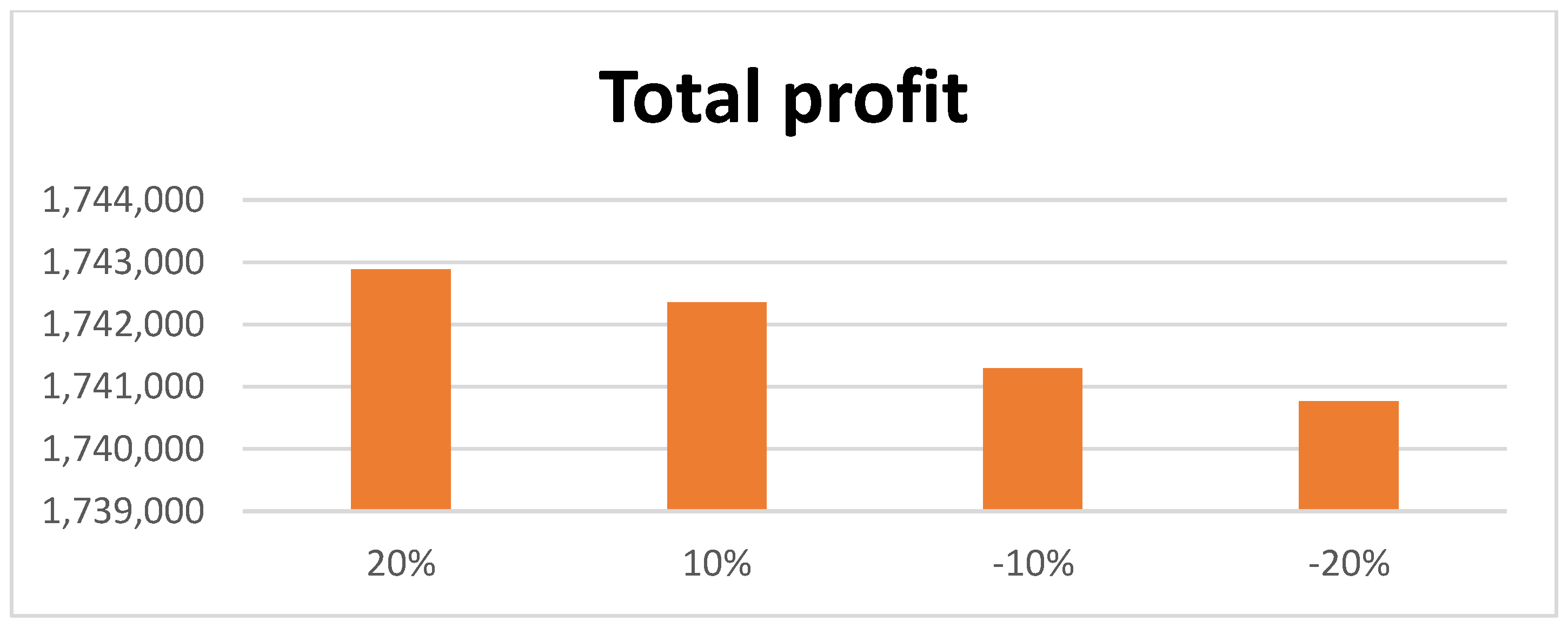
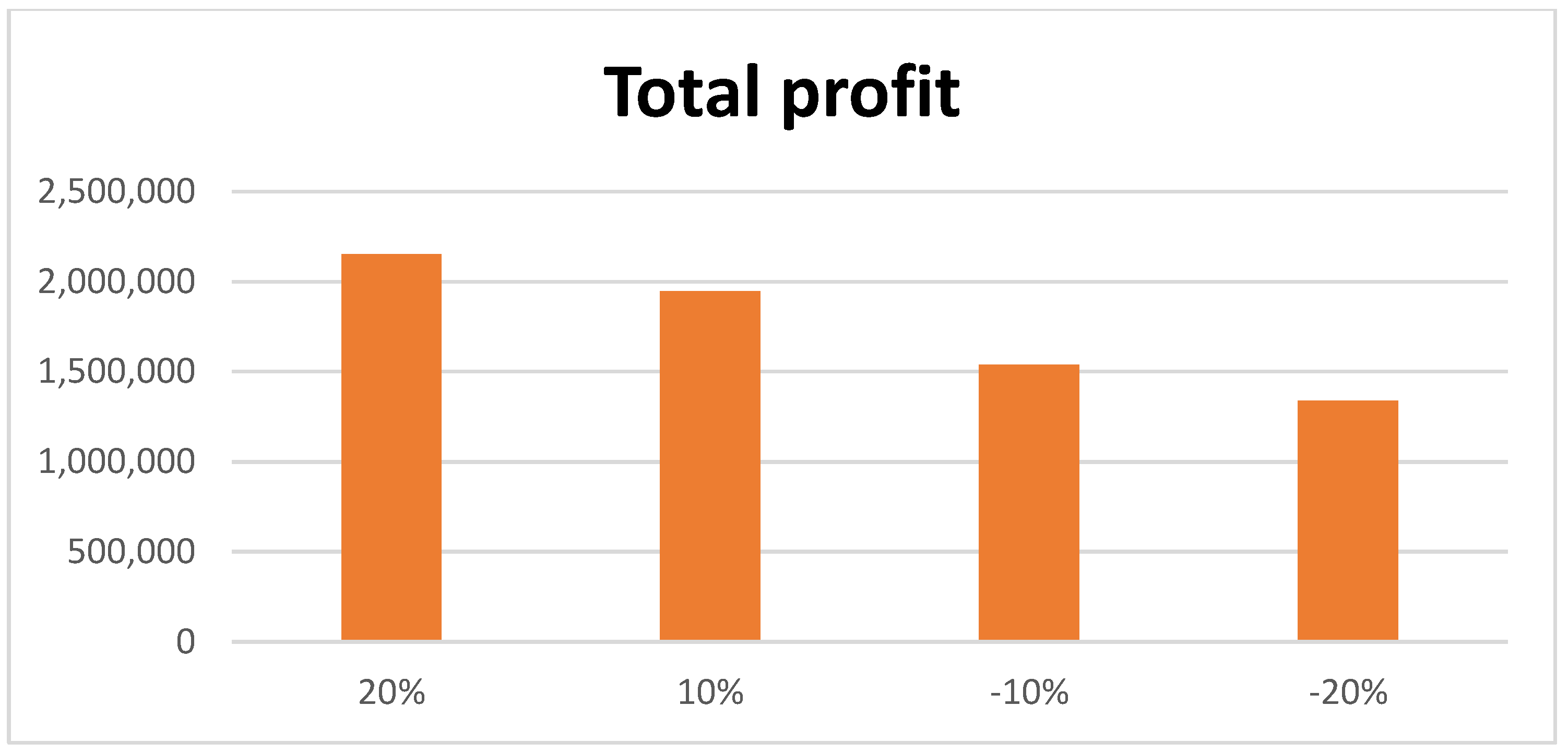
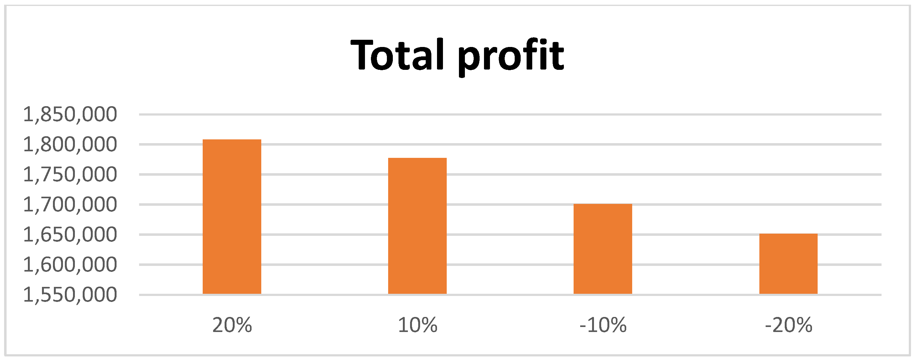
• In this model, only one company produces inventory and then supplies it to multiple buyers. Here, each buyer has a separate organization with a different number of possible suppliers. It was found through sensitivity analysis that, for the first supplier of the first group of buyers, if the value of the selling price is increased to a maximum of 20 percent, the production time is reduced. Additionally, the maximum profit of USD 233 is obtained by reducing the delivery time given to the buyer and the supplier. Conversely, by reducing the value of the selling price, all types of time periods increase, and a small amount of profit also increases.
• If the value of the selling price for the second supplier of the first group is increased slightly by about 20 percent, then it is observed that the total profit increases by USD 210 with a decline in the production time. Conversely, if the value of the selling price declines by about 20 percent, then the total profit is reduced by USD 210, increasing the production time to 16 days.
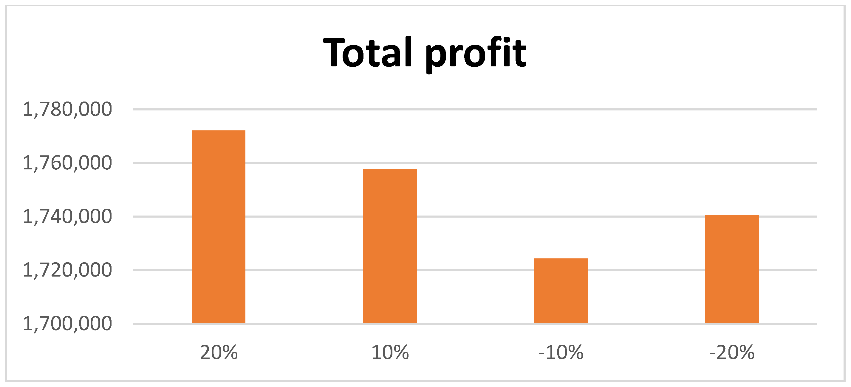
• A total reduction of 31 days in the production time upon increasing the selling price of the first supplier from the second group of suppliers and a decrease of 16 days in the first delivery time from producer to buyer, plus a USD 466 increase in total profit, were found. In addition, the increase in the selling price for another supplier in the second group resulted in an increase of 83 days in production time and an increase in total profit by USD 541. In contrast, for all suppliers in the other group, the selling price is reduced by about 20 percent; total profit also increases, along with an increase in working hours for all supply chain members, indicating lower profit.
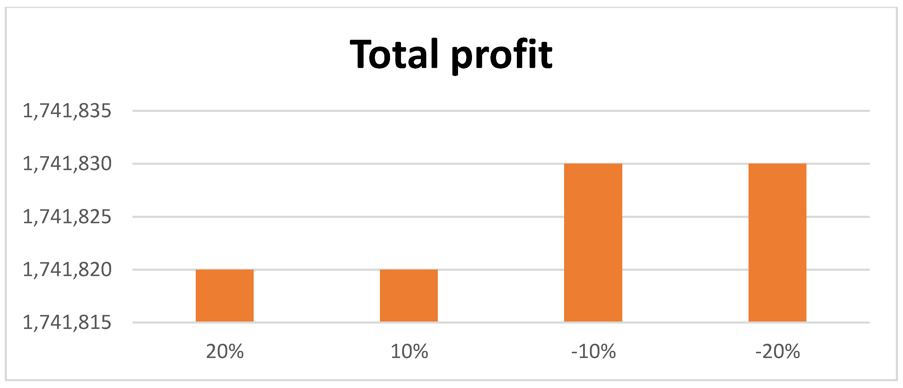
• When vaccines are manufactured and supplied to all the buyers from the production house, the job of the buyer is to deliver the vaccine to the supplier very quickly. This requires taking into account the total number of shipments delivered from the buyer to the supplier, and if the total number of shipments is increased to a maximum of 20 percent, then it is found that the production period is 93 days, with a deficiency of USD 131 in total profit. In addition, if the number of shipments is reduced by 20 percent, a profit of USD 164 is observed. It is concluded that if the total number of shipments in delivering the vaccine to the supplier is minimized, the maximum profit is obtained.
• When the vaccine is manufactured, special attention is given to the production plant to ensure that the minimum quantity of inventory becomes spoiled. In that case, it becomes the producer’s responsibility to maintain the inventory. To ensure that the lost quantity is minimized, he sees a slight variation in his holding cost in holding the inventory. If the holding cost is increased by 20 percent, then there is a very small difference in total profit, but if the holding cost is reduced by 20 percent, then there is a slight increase in total profit.
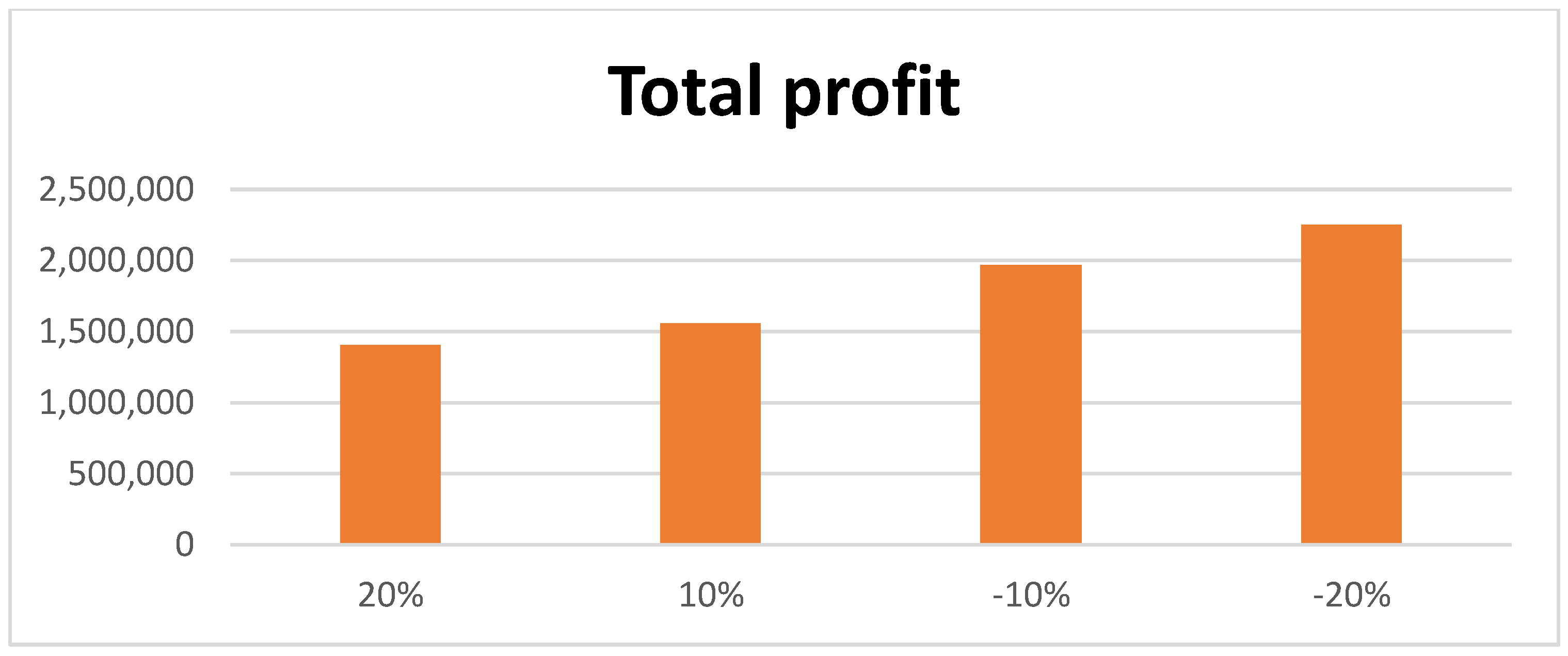
• Additionally, an examination of the sensitivity of the deteriorating rate of inventory for each member of the supply chain found that if the supplier’s deterioration rate increased by 20 percent, the overall profit declined. Conversely, increasing the deterioration rate of the buyer and supplier by 20 percent will see an increase of USD 65 and USD 114 in total profit.

6. Conclusions

This study has developed a supply chain model through which inventory can be delivered to every citizen as early as possible. Here, there is a producer and multiple buyers, and each buyer has their own separate group in which multiple suppliers have been taken. Inflation is also added to the model for inflationary fluctuations. To understand this model in real life, a numerical example has been discussed, and the total profit from the supply chain has been extracted. Through this study, it is concluded that the total profit is found to be at a maximum when the selling price of the producer, buyer, and supplier is increased by 20 percent. To achieve the maximum profit, the total number of shipments from the buyer to the supplier must be reduced. To reduce the transportation cost, the cost of the producer of keeping the inventory safe will also have to be reduced.

The important conclusions observed in this model are as follows: If a reduction in the inflation rate is assumed, then there is an increase in the total profit; conversely, if there is an increase in the inflation rate, then the total profit continuously decreases. The biggest advantage of this research is for those countries who are ready to complete vaccine manufacturing quickly and to reach the last member of the supply chain to improve their country’s economy.

This study was conducted for deteriorated items with multiple players. Thus, a non-deteriorating item is one of the limitations of this study. Instead of fixed ordering costs, one can extend this study by considering variable ordering costs. Fixed demand is another limitation of this study. In the future, one can extend this study by considering variable demand and flexible production rates with remanufacturing. Different carbon emission policies can be adopted to reduce carbon emissions, and some investments can be incorporated to enhance the product’s greenness, which will be an interesting research direction in the future. On the other hand, considering a fuzzy uncertain environment can extend this study.

References

1. Asghar, I.; Kim, J.S. An automated smart EPQ based inventory model for technology dependent product under stochastic failure and repair rate. Symmetry 2020, 12, 388. [Google Scholar] [CrossRef] [Green Version]
2. Mallick, R.K.; Patra, K.; Mondal, S.K. Mixture inventory model of lost sale and back order with stochastic lead time demand on permissible delay in payments. Ann. Oper. Res. 2020, 292, 341–369. [Google Scholar] [CrossRef]
3. Mashud, A.H.; Roy, D.; Daryanto, Y.; Ali, M.H. A sustainable inventory model with imperfect products, deterioration, and controllable emissions. Mathematics 2020, 8, 2049. [Google Scholar] [CrossRef]
4. Bachar, R.K.; Bhuniya, S.; Ghosh, S.K.; Sarkar, B. Controllable energy consumption in a sustainable smart manufacturing model considering superior service, flexible demand, and partial outsourcing. Mathematics 2022, 10, 4517. [Google Scholar] [CrossRef]
5. Sarkar, B.; Kar, S.; Basu, K.; Guchhait, R. A sustainable managerial decision-making problem for a substitutable product in a dual-channel under carbon tax policy. Comput. Ind. Eng. 2022, 172, 108635. [Google Scholar] [CrossRef]
6. Rau, H.; Wu, M.Y.; Wee, H.M. Integrated inventory model for deteriorating items under a multi-echelon supply chain environment. Int. J. Prod. Econ. 2003, 86, 155–168. [Google Scholar] [CrossRef]
7. Rani, S.; Ali, R.; Agarwal, A. Inventory model for deteriorating items in green supply chain with credit period dependent demand. Int. J. Appl. Eng. Res. 2020, 15, 157–172. [Google Scholar]
8. Shaikh, A.K.; Panda, G.C.; Khan, M.A.; Mashud, A.H.; Biswas, A. An inventory model for deteriorating items with preservation facility of ramp type demand and trade credit. Int. J. Oper. Res. 2020, 17, 514–551. [Google Scholar] [CrossRef]
9. Gupta, M.; Tiwari, S.; Jaggi, C.K. Retailer’s ordering policies for time varying deteriorating items with partial backlogging and permissible delay in payments in a two warehouse environment. Ann. Oper. Res. 2020, 295, 139–161. [Google Scholar] [CrossRef]
10. Padiyar, S.V.S.; Kuraie, V.; Bhagat, N.; Singh, S.R.; Dem, H. Green integrated model for imperfect production process under reliability. J. Math. Control Sci. Appl. 2022, 8, 1–13. [Google Scholar]
11. Hasan, K.W. A production inventory model for the deteriorating goods under COVID-19 disruption risk. World J. Adv. Res. Rev. 2022, 13, 355–368. [Google Scholar] [CrossRef]
12. Kumar, N.; Dahiya, S.; Kumar, S. An Inventory Model deteriorating items with Demand Dependent Production Rate under Permissible Delay Payment. Turk. J. Comput. Math. Educ. (TURCOMAT) 2022, 13, 226–253. [Google Scholar]
13. Chou, T.H. Integrated Two-Stage Inventory Model for Deteriorating Items. Master’s Thesis, Chung Yuan Christian University, Taoyuan City, Taiwan.
14. Rani, M.; Kishan, H. A multi echelon supply chain inventory model with variable demand rate for deteriorating items. Pure Appl. Math. Sci. 2011, LXXIV, 31–44. [Google Scholar]
15. Habib, M.S.; Omair, M.; Ramzan, M.B.; Chaudhary, T.N.; Farooq, M.; Sarkar, B. A robust possibilistic flexible programming approach toward a resilient and cost-efficient biodiesel supply chain. J. Clean Prod. 2022, 366, 132752. [Google Scholar] [CrossRef]
16. Jaggi, C.K.; Pareek, S.; Sharma, N.; Nidhi. Fuzzy inventory model for deteriorating items with time varying demand and shortage. Am. J. Oper. Res. 2012, 2, 81–92. [Google Scholar] [CrossRef]
17. Barman, H.; Parvin, M.; Roy, S.K.; Weber, G.W. Back-ordered inventory model with inflation in a cloudy-fuzzy environment. J. Ind. Manag. Optim. 2021, 17, 1913–1941. [Google Scholar] [CrossRef] [Green Version]
18. Rana, R.S.; Kumar, D.; Prasad, K. Two warehouse dispatching policies for perishable items with freshness efforts, inflationary conditions and partial backlogging. Oper. Manag. Res. 2022, 15, 28–45. [Google Scholar] [CrossRef]
19. Sarkar, B.; Joo, J.; Kim, Y.; Park, H.; Sarkar, M. Controlling defective items in a complex multi-phase manufacturing system. Rairo-Oper. Res. 2022, 56, 871–889. [Google Scholar] [CrossRef]
20. Maihami, R.; Govindan, K.; Fattahi, M. The inventory and pricing decisions in a three-echelon supply chain of deteriorating items under probabilistic environment. Transp. Res. Part E Logist. Transp. Rev. 2019, 131, 118–138. [Google Scholar] [CrossRef]
21. Sarkar, B.; Dey, B.K.; Sarkar, M.; Kim, S.J. A smart production system with an autonomation technology and dual channel retailing. Comput. Ind. Eng. 2022, 173, 108607. [Google Scholar] [CrossRef]
22. Jiang, Y.; Zhao, Y.; Dong, M.; Han, S. Sustainable supply chain network design with carbon footprint consideration: A case study in China. Math. Probl. Eng. 2019, 2019, 3162471. [Google Scholar] [CrossRef]
23. Sebatjane, M.; Adetunji, O. A three echelon supply chain for economic growing quantity model with Price and freshness dependent demand: Pricing, ordering, and shipment decisions. Oper. Res. Perspect. 2020, 7, 100153. [Google Scholar] [CrossRef]
24. Sana, S.S. A structural mathematical model on two echelon supply chain system. Ann. Oper. Res. 2021, 315, 1997–2025. [Google Scholar] [CrossRef]
25. Lu, C.J.; Lee, T.S.; Gu, M.; Yang, C.T. A multistage sustainable production inventory model with carbon emission reduction and Price dependent demand under Stackelberg game. Appl. Sci. 2020, 10, 4878. [Google Scholar] [CrossRef]
26. Jauhari, W.M.; Adam, N.A.F.P.; Rosyidi, C.N.; Pujawan, N.; Shah, N.H. A closed loop supply chain model with rework, waste disposal, and carbon emissions. Oper. Res. Perspect. 2020, 7, 100155. [Google Scholar] [CrossRef]
27. Padiyar, S.V.S.; Singh, S.R.; Punetha, N. Inventory system with price dependent consumption for deteriorating items with shortages under fuzzy environment. Int. J. Sustain. Manag. Inform. 2021, 7, 218–231. [Google Scholar] [CrossRef]
28. Karimi, M.; Sadjadi, S.J. Optimization of a multi-item inventory model for deteriorating items with capacity constraint using dynamic programming. J. Ind. Manag. Optim. 2022, 18, 1145. [Google Scholar] [CrossRef]
29. Tiwari, S.; Cárdenas-Barrón, L.E.; Khanna, A.; Jaggi, C.K. Impact of trade credit and inflation on retailer’s ordering policies for non-instantaneous deteriorating items in a two-warehouse environment. Int. J. Prod. Econ. 2016, 176, 154–169. [Google Scholar] [CrossRef]
30. Mukherjee, T.; Sangal, I.; Sarkar, B.; Alkadash, T.M. Mathematical estimation for maximum flow of goods within a cross-dock to reduce inventory. Math. Biosci. Eng. 2022, 19, 13710–13731. [Google Scholar] [CrossRef]
31. Mahapatra, A.S.; Dasgupta, A.; Shaw, A.K.; Sarkar, B. An inventory model with uncertain demand under preservation strategy for deteriorating items. Rairo-Oper. Res. 2022; in press. [Google Scholar] [CrossRef]
32. Palanivel, M.; Uthayakumar, R. Two-warehouse inventory model for non–instantaneous deteriorating items with optimal credit period and partial backlogging under inflation. J. Control Decis. 2016, 3, 132–150. [Google Scholar] [CrossRef]
33. Singh, S.; Sharma, S.; Pundir, S.R. Two-warehouse inventory model for deteriorating items with time dependent demand and partial backlogging under inflation. Int. J. Math. Model. Comput. 2018, 08, 73–88. [Google Scholar]
34. Agarwal, A.; Sangal, I.; Singh, S.R.; Rani, S. Two warehouse inventory model for lifetime deterioration and inflation with exponential demand and partial lost sales. Int. J. Pure Appl. Math. 2018, 118, 1253–1265. [Google Scholar]
35. Singh, S.R.; Rana, K. Effect of inflation and variable holding cost on life time inventory model with multi variable demand and lost sales. Int. J. Recent Technol. Eng. 2020, 8, 5513–5519. [Google Scholar] [CrossRef]
36. Alamri, O.A.; Jayaswal, M.K.; Khan, F.A.; Mittal, M. An EOQ Model with Carbon Emissions and Inflation for Deteriorating Imperfect Quality Items under Learning Effect. Sustainability 2022, 14, 1365. [Google Scholar] [CrossRef]
37. Alfares, H.K.; Attia, A.M. A supply chain model with vendor-managed inventory, consignment, and quality inspection errors. Int. J. Prod. Res. 2017, 55, 5706–5727. [Google Scholar] [CrossRef]
38. Jaggi, C.K.; Aggarwal, K.K.; Goel, S.K. Optimal order policy for deteriorating items with inflation induced demand. Int. J. Prod. Econ. 2006, 103, 707–714. [Google Scholar] [CrossRef]
39. Padiyar, S.V.S.; Kuraie, V.C.; Rajput, N.; Padiyar, N.B.; Joshi, D.; Adhikari, M. Production inventory model with limited storage problem for perishable items under learning and inspection with fuzzy parameters. Des. Eng. 2021, 9, 12821–12839. [Google Scholar]
40. Aghighi, A.; Goli, A.; Malmir, B.; Trikolaee, E.B. The stochastic location-routing-inventory problem of perishable products with reneging and balking. J. Ambient Intell. Hum. Comput. 2021, in press. [CrossRef]
41. Goli, A.; Ala, A.; Mirjalili, S. A robust possibilistic programming framework for designing an organ transplant supply chain under uncertainty. Ann. Oper. Res. 2022, in press. [CrossRef]
42. Tirkolaee, E.B.; Aydin, N.S. Integrated design of sustainable supply chain and transportation network using a fuzzy bi-level decision support system for perishable products. Expert Syst. Appl. 2022, 195, 116628. [Google Scholar] [CrossRef]
43. Tirkolaee, E.B.; Goli, A.; Mardani, A. A novel two-echelon hierarchical location-allocation-routing optimization for green energy-efficient logistics systems. Ann. Oper Res. 2021, in press. [CrossRef]
44. Alinezhad, M.; Mahdavi, I.; Hematian, M.; Trikolaee, E.B. A fuzzy multi-objective optimization model for sustainable closed-loop supply chain network design in food industries. Environ. Dev. Sustain. 2022, 24, 8779–8806. [Google Scholar] [CrossRef]
45. Sarkar, B.; Ganguly, B.; Pareek, S.; Cárdenas-Barrón, L.E. A three-echelon green supply chain management for biodegradable products with three transportation modes. Comput. Ind. Eng. 2022, 174, 108727. [Google Scholar] [CrossRef]
46. Padiyar, S.V.S.; Vandana, V.; Bhagat, N.; Singh, S.R.; Sarkar, B. Joint replenishment strategy for deteriorating multi-item through multi-echelon supply chain model with imperfect production under imprecise and inflationary environment. Rairo-Oper. Res. 2022, 56, 3071–3096. [Google Scholar] [CrossRef]
47. Mahapatra, A.S.; Mahapatra, M.S.; Sarkar, B.; Majumder, S.K. Benefit of preservation technology with promotion and time-dependent deterioration under fuzzy learning. Expert Syst. Appl. 2022, 201, 117169. [Google Scholar] [CrossRef]
48. Fallah, M.; Nozari, H. Neutrosophic mathematical programming for optimization of multi-objective sustainable biomass supply chain network design. CMES-Comp. Model. Eng. Sci. 2021, 129, 927–951. [Google Scholar] [CrossRef]
49. Sundararajan, S.; Vaithyasubramanian, S.; Rajinikannan, M. Price determination of a non-instantaneous deteriorating EOQ model with shortage and inflation under delay in payment. Int. J. Syst. Sci.-Oper. Logist. 2022, 9, 384–404. [Google Scholar] [CrossRef]
50. Gupta, S.; Vijaygargy, L.; Sarkar, B. A bi-objective integrated transportation and inventory management under a supply chain network considering multiple distribution networks. Rairo-Oper. Res. 2022, 56, 3991–4022. [Google Scholar] [CrossRef]
51. Khan, M.A.A.; Shaikh, A.A.; Cárdenas-Barrón, L.E.; Mashud, A.H.M.; Treviño-Garza, G.; Céspedes-Mota, A. An Inventory Model for Non-Instantaneously Deteriorating Items with Nonlinear Stock-Dependent Demand, Hybrid Payment Scheme and Partially Backlogged Shortages. Mathematics 2022, 10, 434. [Google Scholar] [CrossRef]
52. Dey, B.K.; Yilmaz, I.; Seok, H. A sustainable supply chain integrated with autonomated inspection, flexible eco-production, and smart transportation. Processes 2022, 10, 1775. [Google Scholar] [CrossRef]
53. Chakraborty, D.; Jana, D.K.; Roy, T.K. Multi-warehouse partial backlogging inventory system with inflation for non-instantaneous deteriorating multi-item under imprecise environment. Soft Comput. 2020, 24, 14471–14490. [Google Scholar] [CrossRef]
54. Khan, M.A.A.; Halim, M.A.; AlArjani, A.; Shaikh, A.A.; Uddin, M.S. Advance and delay in payments with the price-discount inventory model for deteriorating items under capacity constraint and partially backlogged shortages. Alex. Eng. J. 2022, 61, 1735–1745. [Google Scholar]
55. Duary, A.; Das, S.; Arif, M.G.; Abualnaja, K.M.; Khan, M.A.A.; Zakarya, M.; Shaikh, A.A. Inventory management with hybrid cash-advance payment for time-dependent demand, time-varying holding cost and non-instantaneous deterioration under backordering and non-terminating situations. Alex. Eng. J. 2022, 61, 8469–8486. [Google Scholar]
56. Shah, N.H.; Naik, M.K. Inventory policies for deteriorating items with time-price backlog dependent demand. Int. J. Syst. Sci.-Oper. Logist. 2020, 7, 76–89. [Google Scholar] [CrossRef]
Figure 1. Concavity of the total profit function with respect to time T1.
Mathematics 11 00104 g001
Figure 2. Concavity of the total profit function with respect to time T.
Mathematics 11 00104 g002
Figure 3. Total profit versus σ 11 .
Mathematics 11 00104 g003
Figure 4. Total profit versus σ 12 .
Mathematics 11 00104 g004
Figure 5. Total profit versus σ 21 .
Mathematics 11 00104 g005
Figure 6. Total profit versus σ 22 .
Mathematics 11 00104 g006
Figure 7. Total profit versus r.
Mathematics 11 00104 g007
Figure 8. Total profit versus hp.
Mathematics 11 00104 g008
Figure 9. Total profit versus θ 1 .
Mathematics 11 00104 g009
Figure 10. Total profit versus θ 2 .
Mathematics 11 00104 g010
Figure 11. Total profit versus θ 3 .
Mathematics 11 00104 g011