Abstract
Cell-like P systems with channel states and symport/antiport rules (CCS P systems) are a type of nondeterministic parallel biological computing model, where there exists a channel between adjacent regions and there is a state on each channel to control the execution of symport/antiport rules. In this work, a synchronization rule is introduced into CCS P systems, a variant of CCS P systems called CCS P systems with synchronization rule (CCSs P systems) is proposed. The universality of CCSs P systems with only uniport (symport or antiport) rules is investigated. By simulating the register machine, we proved that CCSs P systems have the ability to simulate any Turing machine in the following three cases: having two membranes, two channel states and using symport rules of length at most 2; having one membrane, three channel states and using symport rules of length at most 2; and having one membrane, two channel states and using antiport rules of length at most 3.
Keywords:
bio-inspired computing; membrane computing; cell-like P systems; channel states; synchronization rule; universality MSC:
68Q05; 68Q10; 68Q85
1. Introduction
In recent years, with the development of science and technology, computer science plays an important role in our contemporary life. However, in the area of computer science, biology has had a significant effect on the course of its development. Many computing ideas, models and methods are inspired by biological phenomena, such as membrane computing [1], genetic algorithm (evolutionary computing) [2] and neural computing [3], which are familiar to everyone in natural computing.
Since membrane computing was proposed by Păun in the late 1990s, a kind of computational model has been abstracted from the structure and function of living cells, and these computing models are called membrane systems (also known as P systems). After more than twenty years of development, many variants of P systems have been proposed and investigated, which involve theoretical research [4,5,6,7] and application [8,9,10]. According to the structure of membranes, there are three main computing models that have been extensively studied: cell -like membrane systems [11] (consisting of main membrane and the membranes arranged in hierarchical structure within the main membrane); tissue-like membrane systems [12] (having several single-membrane cells in a tissue, inspired by the communication between cells in the tissue) and neural-like membrane systems (a neural network, inspired by the way that neurons send short electrical pulses at precise times and other neurons communicate with each other) [13]. The readers can visit the website of P systems http://ppage.psystems.eu (accessed on 3 September 2022) to obtain some information about membrane computing.
Cell-like P systems are composed of the main membrane and some inner membranes arranged according to the hierarchical structure. These membranes divide the interior of a cell into several regions. Each region contains multiple sets of objects and rules. Objects can be evolved according to the rules in the region. Supposing that there are no other membranes in a membrane, it is called an elementary membrane, otherwise, it is called a non-elementary membrane. The outermost main membrane is called the skin membrane (also known as the superficial membrane), and the space beyond the skin membrane is called the environment. The structure of cell-like P systems is shown in Figure 1. The forms of rules include rewriting (evolutionary) rules [14], communication (symport/antiport) rules [15], a symport rule is (u, in) or (u, out), which means that object u can enter or leave the current membrane. An antiport rule is (u, in; v, out), which means that object u enters the membrane and object v is sent out of the membrane. The length of a communication rule is the total number of objects participating in rules.
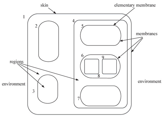
Figure 1.
A cell-like P system structure.
Inspired by a variety of biological phenomena, many variants of cell-like P systems have been proposed and investigated. For example, the concept of channel states was put forward in the literature [16], introducing this concept to cell-like P systems. Thus, a variant of the cell-like systems, called cell-like P systems with channel states and symport/antiport (CCS P systems, for short) was proposed. There is a channel between two cells or cell and the environment, each channel corresponds to a state, which is used to control the use of communication rules. During the use of rules, the state may change or may not change. In addition, objects can change when moving from one region to another. Readers can refer to [17,18,19] for more detailed information about channel states and evolution symport/antiport rules; according to [20], it can be known that proteins can exist on cells, and the computational power of cell-like P systems with one protein on membranes was obtained [21].
It is well known that membrane systems can work in different ways, for instance, Maximal parallelism [22,23] is the most common working mode for P systems. In each step of evolution, as long as the objects that can evolve must complete evolution, there is no limit to the number of times the rules can be used; Minimal parallelism [24], it means that at least one rule is used in each step of computation as long as there are applicable rules on each membrane (more rules are used, but we do not care how many rules are used); Flat maximum parallelism [25,26,27] is that in every step of computation, we must select the maximum set of an effective rule, and each rule in this rule set can only be used exactly once; asynchronous mode [28], it means that any number of rules associated with a region can be applied in one derivation step; synchronization rule is an interesting rule application strategy, which was first put forward in [29]. In synchronization rule mode, we first give some synchronization sets of rules [30], a rule in a synchronization set of rules can be used only if the synchronization rule set is enabled. In other words, all rules in the synchronization set are enabled, it is impossible to use one rule in the synchronization set alone.
The computational power of CCS P systems has been proved in [17], however, it is a motivation whether CCS P systems with synchronization sets of rules, working in a maximally parallel manner, are Turing universal. In this paper, a control mechanism of rules, synchronization sets of symport/antiport rules are considered. We propose a variant of cell-like P systems, called cell-like P systems with channel states and synchronization rule (CCSs P systems, for short), and investigate the computational power of CCSs P systems. The main contributions of this article are as follows.
- (1)
- Synchronization symport/antiport rule modes are introduced into cell-like P systems with channel states, based on sets of synchronization rule, cell-like P systems with channel state working in synchronization rule mode are proposed.
- (2)
- The computational power of CCSs P systems is investigated, we prove that CCSs P systems are as powerful as Turing machines in the following three cases: CCSs P systems with two membranes, two channel states and the length of symport rules is at most 2; CCSs P systems consist of only one membrane, two channel states and antiport rules of length at most 3; CCSs P systems with one membrane, three channel states and symport rules of length at most 2.
- (3)
- It is known that cell-like P systems with at least two channel states and using uniport rules are able to compute only finite sets of non-negative integers. If cell-like P systems with two membranes and only using symport rules of length at most 2, at least four channel states must be included for such P systems to be Turing universal. In addition, cell-like P systems with one membranes, only if using both symport rules of length at most 1 and antiport rules of length at most 2, are Turing universal. However, the results obtained in this work show that synchronization rule can increase the computational power of CCSs P systems.
2. Preliminaries
Firstly, some of basic concepts and symbols of formal language related with CCSs P systems are introduced in this section. The reader can also refer to [31,32] for more detailed information.
An alphabet V contains a finite non-empty set of objects, represents the set of all strings that are made up of objects from V, in other words, is called the free monoid produced by the join operation on V (the unit of the free monoid is ). The empty string is represented by , the set of non-empty strings over V, i.e., , is denoted by .
In mathematics, for a given set, if the same object in the set appears more than once, the number of each object in the set is defined as the of the object, and the set is called a . For example, a denoted by can be defined as a two-tuples , where , is the set of natural numbers, f is a mapping from V on the set of natural numbers N. For an object , we use to denote this object, where is the number of object a. Assuming that the alphabet , then the can be represented as . We use to represent the set of all finite non-empty over V.
A register machine is a tuple , where:
- m is the number of register machine;
- H is the set of instruction labels;
- are different instruction labels, where is the initial instruction label, and is the halt instruction label;
- I is the set of program instruction label, and follows the following form (Each label in H marks only one instruction in I to accurately identify it):
- −
- (add 1 to register machine r, then nondeterministically select either instruction or instruction );
- −
- (If register r is non-empty, then register r minus 1 to instruction label , otherwise to instruction label );
- −
- : the halt label instruction.
Initially, all registers in the register machine M are empty, that is, each register stores the number 0. When the register machine starts working, the initial instruction is executed first, then the other instructions (ADD instructions and SUB instructions) are executed successively. At some point, if the halt instruction is executed, the computation stops. The number computed by M stored in the first register is regarded as the computing result and output, a set of all numbers computed by the register machine M is denoted by .
It is well known that a register machine is a kind of abstract machine used in formal logic and theoretical computer science, which is equivalent to a Turing machine. The family of all recursively enumerable natural numbers calculated by Turing machines is represented by , so both register machines and Turing machines can characterize . More information and theories related to Turing machines and register machines, readers can refer to [33].
3. The Model Description of CCSs P Systems
In this section, we give the definition of cell-like P systems with channel states and synchronization rule.
A cell-like P system with channel states and sets of synchronization rules, of degree , is a tuple. where
- V is a finite non-empty set, called alphabet of objects;
- K is an alphabet of channel states, it is disjoint of V;
- is a multiple set of objects, each object of is initially stored in the environment;
- represents the membrane structure of the system , it has q membranes that are related to each other, and labeled by ;
- (), initially placed in every membrane, are finite of objects over V;
- () represent initial channel states of region i;
- () are finite sets of rules exist in region i, which cover the following forms:
- −
- Symport rules: or , for , , ;
- −
- Antiport rules: , for , , , ;
- , where is a set of all rules in the system , is the set of all subsets of , is the set of synchronization rules, which is also composed of some rules in ;
- is the output region.
According to the above definition, the system consists of q membranes, the region between each two membranes is represented by different label i (), and the environment is labeled by 0. Each membrane of this system has its membrane and membrane, for instance, the membrane of the skin membrane 1 is the environment and the membrane is membrane 2, and so on. The length of a symport rule or is defined as , and the length of an antiport rule is defined as .
A symport rule of () or is applied-that means the object u is moved into its inner membrane i from the parent membrane ( represents object u is moved from the environment to membrane 1) or moved into the parent membrane from the present membrane i ( represents object u is sent out of membrane 1 and into the environment), as well as the state between parent membrane and membrane i is changed from s to .
An antiport rule of () is used. This means the object u is moved into membrane i from its parent membrane, meanwhile the object v is sent out of membrane i and into its parent membrane, represents object u is moved into membrane 1 from the environment and object v is sent out of membrane 1 and into the environment, as well as the state between parent membrane and membrane i is changed from s to .
In this paper, the set of synchronization symport/antiport rules are considered, that is, for a finite set of rules in a region, some of symport/antiport rules in the set are grouped into some new sets of rules, these new sets are referred to as synchronous sets. At some step, a rule in a synchronous set can be available only if all rules in the set are used synchronously, as long as one rule is unavailable, all rules including available rules in the set cannot be used. In addition, all available rules in a finite set of rules and in a synchronous set are chosen and applied as many times as possible in a maximally parallel mode.
A configuration of cell-like P systems with channel states and synchronization rules can be defined at any time as multiple sets of all objects over V in each region, and channel states associated with each membrane. The multiple sets of objects over at any time in the environment. Assume that the multiple set of objects in the environment has an infinite number of copies and can not be changed through the computation, then the initial configuration of the system is .
The computation of system includes a sequence of consecutive configurations, starting from the initial configuration and ending with the halting configuration (no applicable rules are enabled at some step in the system), a transition means the computation from one configuration to another. A computation stops when the system reaches the halting configuration, a result computed by the system is given, which refers to the number of copies of objects located in region .
All results computed by a CCSs P system are represented with . The family of all sets of numbers computed by such a P system can be represented with , where indicate natural number, m refers to the number of membranes in this system , refers to the number of channel states required is k, refers to the maximum length of symport rules is and refers to the maximum length of antiport rules is , indicates that the system works in synchronization rule mode. Note that if only one of symport rules or antiport rules is applied, we replace with or . If any one of the parameters m, k, and is not bounded, it is replaced with ∗.
4. An Example
In this section, we give an example to illustrate how a CCSs P system works in a maximal parallel way and the synchronization rule model, respectively.
Let , where , , .
If the system works in a maximal parallel way, the computing process needs two steps. In the first step, since there are two objects a in membrane 2, two objects a are sent to membrane 1 by using , hence, membrane 1 contains two objects a. After that, the use of rules in the system has the following three cases: (1) only using two times; (2) using and once; (3) only using two times. After two steps, no other rules can be applied and the computing halts. Therefore, the result (the number of object a in membrane 3) calculated by is .
If , that means rules and belong to a synchronization rule set, so and should only be used together, not separately. In this case, at step 1, since there are two objects a in membrane 2, two copies of object a are sent to membrane 1 by using , hence, membrane 1 contains two a. Because and are in the synchronization set of rules, they must be used at the same time at step 2. After two steps, no other rules can be applied amd the computing halts. Therefore, the result (the number of object a in membrane 3) calculated by is only 1.
5. The Computational Power of CCSs P Systems
The universality of cell-like P systems with channel states and symport/antiport rules was studied in [17]. It was proved that channel states can improve the computational power of CCS P systems. In this section, we investigate the computational power of cell-like P systems with channel states and synchronization symport/antiport rules, and prove that the use of synchronization rules sets can also increase the universality of cell-like P systems with channel states.
The Church–Turing thesis states that any computation or algorithm can be performed by a Turing machine. A computer program written in any regular programming language can be translated into a Turing machine, and any Turing machine can be translated into programs in most programming languages [34]. Thus, in the following work, we only need to prove that CCSs P systems can simulate a register machine, and the opposite conclusion can be obtained by Church–Turing thesis.
Theorem 1.
.
Proof.
Here, we only need to prove the inclusion , the reverse inclusion relation can be directly derived from the Church–Turing thesis.
A cell-like P system with channel states and synchronization rules is constructed to simulate the register machine M, which has two membranes, two channel states and only use symport rules of length at most 2, simultaneously, three sets of synchronization rule sets are adopted.
where
- ;
- ;
- ;
- ;
- , and , are described as follows.
- For each ADD instruction of M, we construct the following rules in :;;;;.
The system simulates an ADD instruction in four steps. At step 1, the rule is applied, objects are sent to the environment from membrane 1 and the state does not change between membrane 1 and environment. At step 2, as appears in the environment, by using rule , are brought into membrane 1 from the environment, and the state from s to . At step 3, because the state between the environment and membrane 1 becomes , is once again sent to the environment and the state remains the same. In the fourth step, or is a non-deterministic choice, or are sent to membrane 1 and the state returns to s. Hence, the system can correctly simulate the ADD instruction of M.
- For each SUB instruction of M,
- −
- we construct the following rules in :;;;;;;;;;;;;where ,,.
- −
- we construct the following rules in :;;;.
The system simulates a SUB instruction in up to seven steps. At step 1, and are sent to environment by using rule , and the state remains the same. At step 2, as appears in the environment, are sent into membrane 1 by using , and the state is changed to between membrane 1 and environment. At step 3, under the influence of state between membrane 1 and the environment, are sent to environment, meanwhile, rule is enabled and used, are sent to membrane 2. At step 4, are sent to membrane 1 and the state also is , simultaneous, is sent to membrane 1 and the state between membrane 2 and membrane 1 is changed to . Then, according to whether there is or not in membrane 1, the following two cases are checked.
- At least one copy of is stored in membrane 1, in this case, it means that the register r is non-empty. At step 5, both rules in membrane 1 and rule in membrane 2 are chosen and used in parallel, objects are sent to membrane 1 by using and the state is changed to s between membrane 1 and environment, at the same time, objects are sent to membrane 1 by using and the state between membrane 1 and membrane 2 is unchanged. At step 6, rule and rule belong to a set of synchronization rule, are sent to the environment from membrane 1 by using , and object is sent to membrane 1 by using rule . Meanwhile, rule is used, object is sent to membrane 2 and the corresponding state is changed to s. At step 7, object presents in the environment, both and are back to membrane 1. After the above simulation process, one copy of object in membrane 1 is reduced by one, and the system will begin to emulate the next instruction (see Table 1).
 Table 1. The application of rules in and , the evolution of channel states and , and the rewriting of multisets and in membrane 1 and 2, respectively. During the simulation of a instruction :() with register r not empty.
 - There is no copy of in membrane 1, that is, the register r is empty. In this case, at step 5, only rule in membrane 2 is enabled, both and are sent to membrane 1. Due to rules and belong to the synchronization rule set, rule cannot be used at step 5, so rule can not be used either. At step 6, both and are applied, objects , and are sent to the environment and the corresponding state is unchanged. Meanwhile, by using rule in , object is sent from membrane 1 to membrane 2, and the state between membrane 1 and membrane 2 is changed to s. At step 7, as exists in the environment, rule is enabled. Since rule and rule in the set of synchronization rule, rule can also be used at this step. Therefore, objects , and are brought back to membrane 1, and the state between membrane 1 and the environment is changed to s, the system will begin to simulate the instruction (see Table 2).
Table 2. The application of rules in and , the evolution of channel states and , and the rewriting of multisets and in membrane 1 and 2, respectively. During the simulation of a instruction :() with register r empty.
Accordingly, the SUB instruction of M is correctly simulated by the system .
The computation stops only when the object appears in the membrane 1 at some point, and there are no rules can be used. The number of copies of object in membrane 1 is regarded as the result calculated by the system , i.e. , which is the end of the proof. □
Theorem 2.
.
Proof.
The inclusion needs to be proved. The reverse inclusion relation can be directly derived from the Church–Turing thesis.
We construct a cell-like P system with channel states and synchronization rules , which consists of only one membrane, two channel states and uses two sets of synchronization antiport rules, to simulate the register machine M.
where
- ;
- ;
- ;
- ;
- , and is described as follows.
- For each ADD instruction of M, we construct the following rules in :;;;;;where .
From the given rules, the system can simply simulate an ADD instruction , which requires three steps. At step 1, rule is applied, both and are sent to the environment from membrane 1, and object is brought into membrane 1 from the environment without changing the state s. Since rule and rule exist in the same set of synchronization rule set, thus rule cannot be used at step 1. At step 2, as object appears in the environment, object brings one copy of object into membrane 1 from the environment by using rule , object is sent back to membrane 1, and the state between membrane 1 and the environment remains s. Synchronously, rule is applied too, object is sent to the environment and object is brought into membrane 1. At step 3, rule or rule is a non-deterministic choice and used, so object brings object or back into membrane 1, and is sent back into the environment. Hence, the next instruction or will be simulated by the system .
- For each SUB instruction of M, we construct the following rules in :;;;;;;;.where .
That the system simulates the SUB instruction is very clear. At step 1, rule is enabled, objects are sent to the environment and object is brought into membrane 1, the corresponding state remains the same. As rule is synchronous with rule , hence, rule can not be applied in the first step. At step 2, as object exists in membrane 1, rules are enabled simultaneously, objects are sent out of membrane 1 and objects are moved into membrane 1 from the environment. Then, we will check if object exists in membrane 1, there are the following two cases.
- If membrane 1 includes at least one copy of , four steps are required to simulate the SUB instruction. At step 3, rule and rule are used in parallel, objects are sent to the environment with one copy of object and objects are brought into membrane 1 and the state is changed from s to between membrane 1 and environment. At step 4, by using rule , objects are brought into membrane 1 and object is sent back into the environment, the state returns to its original state s. In this process, the copy of in membrane 1 is reduced by one, corresponding to the value stored in register 1 is reduced by one. Then the system will begin to simulate the next instruction (see Table 3).
Table 3. The application of rules in , the evolution of channel states , and the rewriting of multisets in membrane 1. During the simulation of a instruction :() with register r not empty.
- If there is no copy of in membrane 1 at this moment, it takes five steps to simulate the SUB instruction. Only rule is enabled at step 3, object in membrane 1 is exchanged with object in the environment and the state becomes between membrane 1 and environment. At step 4, rule is selected and used, and move in opposite directions between membrane 1 and the environment, and the state is changed back to s. At step 5, rule is applied, object is brought into membrane 1 with , and object is released into the environment. Therefore, the system will begin to simulate the next instruction (see Table 4).
Table 4. The application of rules in , the evolution of channel states , and the rewriting of multisets in membrane 1. During the simulation of a instruction :() with register r empty.
Therefore, the SUB instruction of M is correctly simulated by the system .
The computation stops only when the object appears in the membrane 1 at some point, and there are no rules can be used. The number of copies of object in membrane 1 is regarded as the result calculated by the system , i.e. , which is the end of the proof. □
Theorem 3.
.
Proof.
The inclusion needs to be proved. The reverse inclusion relation can be directly derived from the Church–Turing thesis. We construct a cell-like P system with channel states and synchronization rules , which consists of only one membrane, three channel states and uses three sets of synchronization symport rule set, to simulate the register machine M.
where
- ;
- ;
- ;
- ;
- , and is described as follows.
- For each ADD instruction of M, we construct the following rules in :;;;;;
From the given rules, the system can simply simulate an ADD instruction , which requires four steps. At the first step, rule is enabled, objects , are both sent to the environment and the state between the environment and membrane 1 remains constant. At the second step, object is sent back to membrane 1 with one copy of object , and the corresponding state is changed to . At the third step, object is sent to the environment again because rule is available. At the fourth step, both rules and are available, one of them is chosen nondeterministically and used, is sent back to membrane 1 with or , and the state between environment and membrane 1 returns to s. Then, the system will simulate the next instruction or at the next step.
- For each SUB instruction of M, we construct the following rules in :;;;;;;;;;.where ,,.
That the system simulates the SUB instruction is apparent. At step 1, rule is available, objects , are sent out of membrane 1 to the environment and the state between membrane 1 and the environment is still s. Since rule and rule are the same set of synchronization rules, cannot be used at step 1. At step 2, object is sent back to membrane 1 with by using , at the same time, object is sent to the environment by using , and the state between membrane 1 and the environment is changed from s to . Then, we will check if object exists in membrane 1. There are the following two cases:
- If there is at least one copy of object in membrane 1, the process of simulating a SUB instruction requires the following four steps. At step 3, since rule and rule are used in parallel, objects and are sent from membrane 1 to the environment by using . At the same step, object is also sent to the environment by using , and the state between membrane 1 and the environment is changed from to . At step 4, rule and rule are enabled because they belong to the same synchronization rule set, objects , are sent back to membrane 1 with , and the state between membrane 1 and the environment is changed to the original state s. In this case, one copy of object is consumed in membrane 1, corresponding to the register 1 is reduced by one, the system will simulate the next instruction (see Table 5).
Table 5. The application of rules in , the evolution of channel states , and the rewriting of multisets in membrane 1. During the simulation of a instruction :() with register r not empty.
- If there is no copy of object in membrane 1, the simulation of a SUB instruction takes five steps as follows. At step 3, only is used, object is sent to the environment, the state between membrane 1 and the environment is changed to . At step 4, only rule is used, object is sent to the environment and the state between membrane 1 and the environment is changed to . At step 5, since rule and rule are synchronous rule, they are applied at the same time, objects , are brought back to membrane 1 with , as well as the state between membrane 1 and the environment is changed to the original state s. Hence, the system will begin to simulate the next instruction (see Table 6).
Table 6. The application of rules in , the evolution of channel states , and the rewriting of multisets in membrane 1. During the simulation of a instruction :() with register r empty.
Therefore, the SUB instruction of M is correctly simulated by the system .
Only if the object appears in the membrane 1 at some point, there are no rules that can be used and the computation stops. The number of copies of object in membrane 1 is regarded as the result calculated by the system , i.e. , which is the end of the proof. □
6. Conclusions and Future Works
In this paper, sets of synchronization rules are considered in cell-like P systems with channel states. We constructed cell-like P systems with channel states and synchronization rule, and the computational power of such P systems was studied. It is worth mentioning that we proved that cell-like P systems with channel states and using synchronization rules in some cases are Turing universal. For CCS P systems, the number of cells, the number of channel states, and the length of symport/antiport rules are used to describe the complexity of systems. Compared with literature [17], we designed sets of synchronization rules in CCS P systems, the results show that the computational power of CCSs P systems is improved, using synchronization rule sets can increase the computational power of CCS P systems.
There are many variants of membrane systems [35,36,37,38], which are working in a maximally parallel. Considering adding synchronization rule sets to these systems, it is interesting to study the computational power of such P systems.
In addition, it is challenging to solve some NP-complete problems with CCSs P systems by introducing cell division [39,40] or cell separation [41]. For example, SAT problem [42], SUBSET problem [43], Vertex Cover problem [44,45], 3-coloring problem [46] and etc. Some other research topics are to consider synchronization rules in these P systems mentioned above, and to study their computational efficiency.
Author Contributions
Conceptualization, S.J.; writing—original draft preparation, T.L.; material preparation, data collection and analysis were performed by B.X., Z.S. and X.Z.; writing—review and editing, Y.W. All authors have read and agreed to the published version of the manuscript.
Funding
This work was supported by National Natural Science Foundation of China (61902360), the Foundation of Young Key Teachers from University of Henan Province (2019GGJS131), and the Joint Funds of the National Natural Science Foundation of China (U1804262).
Institutional Review Board Statement
Not applicable.
Informed Consent Statement
All authors have checked the manuscript and have agreed to the submission.
Data Availability Statement
Not applicable.
Conflicts of Interest
The authors declare that they have no known competing financial interests or personal relationships that could have appeared to influence the work reported in this paper.
References
- Păun, G. Computing with membranes. J. Comput. Syst. Sci. 2000, 61, 108–143. [Google Scholar] [CrossRef]
- Eiben, A.E.; Schoenauer, M. Evolutionary computing. Inf. Process. Lett. 2002, 82, 1–6. [Google Scholar] [CrossRef]
- Beale, R.; Jackson, T. Neural Computing: An Introduction; CRC Press: Boca Raton, FL, USA, 1990. [Google Scholar]
- Pérez-Jiménez, M.J.; Sosík, P. An optimal frontier of the efficiency of tissue P systems with cell separation. Fundam. Inform. 2015, 138, 45–60. [Google Scholar] [CrossRef]
- Song, B.; Li, K.; Orellana-Martín, D.; Pérez-Jiménez, M.J.; PéRez-Hurtado, I. A survey of nature-inspired computing: Membrane computing. ACM Comput. Surv. 2021, 54, 22. [Google Scholar] [CrossRef]
- Song, T.; Pan, L. Spiking neural P systems with request rules. Neurocomputing 2016, 193, 193–200. [Google Scholar] [CrossRef]
- Wu, T.; Zhang, Z.; Păun, G.; Pan, L. Cell-like spiking neural P systems. Theor. Comput. Sci. 2016, 623, 180–189. [Google Scholar] [CrossRef]
- Peng, H.; Wang, J.; Pérez-Jiménez, M.J.; Wang, H.; Wang, T. Fuzzy reasoning spiking neural P system for fault diagnosis. Inf. Sci. 2013, 235, 106–116. [Google Scholar] [CrossRef]
- Peng, H.; Wang, J.; Pérez-Jiménez, M.J.; Riscos-Núñez, A. An unsupervised learning algorithm for membrane computing. Inf. Sci. 2015, 304, 80–91. [Google Scholar] [CrossRef]
- Zhang, G.; Gheorghe, M.; Pan, L.; Pérez-Jiménez, M.J. Evolutionary membrane computing: A comprehensive survey and new results. Inf. Sci. 2014, 279, 528–551. [Google Scholar] [CrossRef]
- Zandron, C. Bounding the space in P systems with active membranes. J. Membr. Comput. 2020, 2, 137–145. [Google Scholar] [CrossRef]
- Pan, L.; Song, B.; Valencia-Cabrera, L.; Pérez-Jiménez, M.J. The computational complexity of tissue P systems with evolutional symport/antiport rules. Complexity 2018, 2018, 3745210. [Google Scholar] [CrossRef]
- Song, T.; Pan, L. Spiking neural P systems with rules on synapses working in maximum spiking strategy. IEEE Trans. Nanobiosci. 2015, 14, 465–477. [Google Scholar] [CrossRef] [PubMed]
- Păun, A.; Păun, G.; Rozenberg, G. Computing by communication in networks of membranes. Int. J. Found. Comput. Sci. 2002, 13, 779–798. [Google Scholar] [CrossRef]
- Păun, A.; Păun, G. The power of communication: P systems with symport/antiport. New Gener. Comput. 2002, 20, 295–305. [Google Scholar] [CrossRef]
- Freund, R.; Păun, G.; Pérez-Jiménez, M.J. Tissue P systems with channel states. Theor. Comput. Sci. 2005, 330, 101–116. [Google Scholar] [CrossRef]
- Song, B.; Pan, L.; Pérez-Jiménez, M.J. Cell-like P systems with channel states and symport/antiport rules. IEEE Trans. NanoBiosci. 2016, 15, 555–566. [Google Scholar] [CrossRef]
- Song, B.; Pérez-Jiménez, M.J.; Păun, G.; Pan, L. Tissue P systems with channel states working in the flat maximally parallel way. IEEE Trans. NanoBiosci. 2016, 15, 645–656. [Google Scholar] [CrossRef]
- Song, B.; Li, K.; Orellana-Martín, D.; Valencia-Cabrera, L.; Pérez-Jiménez, M.J. Cell-like P systems with evolutional symport/antiport rules and membrane creation. Inf. Comput. 2020, 275, 104542. [Google Scholar] [CrossRef]
- Păun, A.; Păun, M.; Rodríguez-Patón, A.; Sidoroff, M. P systems with proteins on membranes: A survey. Int. J. Found. Comp. Sci. 2011, 22, 39–53. [Google Scholar] [CrossRef]
- Song, B.; Luo, X.; Valencia-Cabrera, L.; Zeng, X. The computational power of cell-like P systems with one protein on membrane. J. Membr. Comp. 2020, 2, 332–340. [Google Scholar] [CrossRef]
- Sburlan, D.Ş. Further results on P systems with promoters/inhibitors. Int. J. Found. Comp. Sci. 2006, 17, 205–221. [Google Scholar] [CrossRef]
- Sburlan, D.Ş. Membrane Computing Insights. In Permitting and Forbidding Contexts; Ovidius University Press: Constanta, Romania, 2012. [Google Scholar]
- Ciobanu, G.; Pan, L.; Păun, G.; Pérez-Jiménez, M.J. P systems with minimal parallelism. Theor. Comput. Sci. 2007, 378, 117–130. [Google Scholar] [CrossRef][Green Version]
- Jiang, S.; Wang, Y.; Xu, F.; Junli, D. Communication P Systems with Channel States Working in Flat Maximally Parallel Manner. Fundam. Informaticae 2019, 168, 1–24. [Google Scholar] [CrossRef]
- Pan, L.; Păun, G.; Song, B. Flat maximal parallelism in P systems with promoters. Theor. Comput. Sci. 2016, 623, 83–91. [Google Scholar] [CrossRef]
- Wu, T.; Jiang, S. Spiking neural P systems with a flat maximally parallel use of rules. J. Membr. Comp. 2021, 3, 221–231. [Google Scholar] [CrossRef]
- Frisco, P.; Govan, G.; Leporati, A. Asynchronous P systems with active membranes. Theor. Comput. Sci. 2012, 429, 74–86. [Google Scholar] [CrossRef][Green Version]
- Aman, B.; Ciobanu, G. Synchronization of rules in membrane computing. J. Membr. Comp. 2019, 1, 233–240. [Google Scholar] [CrossRef]
- Song, B.; Pan, L. Rule synchronization for tissue P systems. Inf. Comp. 2021, 281, 104685. [Google Scholar] [CrossRef]
- Păun, G. Membrane computing. Scholarpedia 2010, 5, 9259. [Google Scholar] [CrossRef]
- Rozenberg, G.; Salomaa, A. (Eds.) Handbook of Formal Languages: Volume 3 Beyond Words; Springer Science & Business Media: Berlin/Heidelberg, Germany, 2012. [Google Scholar]
- Freund, R.; Ibarra, O.H.; Paun, G.; Yen, H.-C. Matrix Languages, Register Machines, Vector Addition Systems; Fénix Editora; Universidad de Sevilla: Sevilla, Spain, 2005. [Google Scholar]
- Clarke, D.A. Computation: Finite and Infinite Machines; Prentice-Hall, Inc.: Englewood Cliffs, NJ, USA, 1968. [Google Scholar]
- Alhazov, A.; Freund, R.; Ivanov, S. Variants of P systems with activation and blocking of rules. Nat. Comp. 2019, 18, 593–608. [Google Scholar] [CrossRef]
- Freund, R.; Rogojin, V.; Verlan, S. Variants of networks of evolutionary processors with polarizations and a small number of processors. Int. J. Found. Comput. Sci. 2019, 30, 1005–1027. [Google Scholar] [CrossRef]
- Orellana-Martín, D.; Valencia-Cabrera, L.; Riscos-Núñez, A.; Pérez-Jiménez, M.J. Minimal cooperation as a way to achieve the efficiency in cell-like membrane systems. J. Membr. Comp. 2019, 1, 85–92. [Google Scholar] [CrossRef]
- Peng, H.; Li, B.; Wang, J.; Song, X.; Wang, T.; Valencia-Cabrera, L.; Pérez-Hurtado, I.; Riscos-Núñez, A.; Pérez-Jiménez, M.J. Spiking neural P systems with inhibitory rules. Knowl.-Based Syst. 2020, 188, 105064. [Google Scholar] [CrossRef]
- Song, B.; Pérez-Jiménez, M.J.; Pan, L. Efficient solutions to hard computational problems by P systems with symport/antiport rules and membrane division. Biosystems 2015, 130, 51–58. [Google Scholar] [CrossRef] [PubMed]
- Song, B.; Li, K.; Zeng, X. Monodirectional evolutional symport tissue P systems with promoters and cell division. IEEE Trans. Parallel Distrib. Syst. 2021, 33, 332–342. [Google Scholar] [CrossRef]
- Jiang, Y.; Zhang, X.; Zhang, Z. A Uniform Solution to Subset Sum by Tissue P Systems with Cell Separation. J. Comput. Theor. Nanosci. 2010, 7, 1507–1513. [Google Scholar] [CrossRef]
- Zandron, C.; Leporati, A.; Ferretti, C.; Mauri, G.; Pérez-Jiménez, M.J. On the computational efficiency of polarizationless recognizer P systems with strong division and dissolution. Fundam. Informaticae 2008, 87, 79–91. [Google Scholar]
- Pérez Jiménez, M.J.; Riscos Núñez, A. Solving the subset-sum problem by P systems with active membranes. New Gener. Comput. 2005, 23, 339–356. [Google Scholar] [CrossRef]
- Díaz Pernil, D.; Pérez Jiménez, M.J.; Riscos Núñez, A.; Romero Jiménez, A. Computational efficiency of cellular division in tissue-like membrane systems. Rom. J. Inf. Sci. Technol. 2008, 11, 229–241. [Google Scholar]
- Krishna, S.N.; Rama, R. A variant of P systems with active membranes: Solving NP-complete problems. Rom. J. Inf. Sci. Technol. 1999, 2, 357–367. [Google Scholar]
- Díaz-Pernil, D.; Gutiérrez-Naranjo, M.A.; Pérez-Jiménez, M.J.; Riscos-Núñez, A. A uniform family of tissue P systems with cell division solving 3-COL in a linear time. Theor. Comput. Sci. 2008, 404, 76–87. [Google Scholar] [CrossRef]

Disclaimer/Publisher’s Note: The statements, opinions and data contained in all publications are solely those of the individual author(s) and contributor(s) and not of MDPI and/or the editor(s). MDPI and/or the editor(s) disclaim responsibility for any injury to people or property resulting from any ideas, methods, instructions or products referred to in the content. |
© 2022 by the authors. Licensee MDPI, Basel, Switzerland. This article is an open access article distributed under the terms and conditions of the Creative Commons Attribution (CC BY) license (https://creativecommons.org/licenses/by/4.0/).