Control of a Hydraulic Generator Regulating System Using Chebyshev-Neural-Network-Based Non-Singular Fast Terminal Sliding Mode Method

Abstract

A hydraulic generator regulating system with electrical, mechanical, and hydraulic constitution is a complex nonlinear system, which is analyzed in this research. In the present study, the dynamical behavior of this system is investigated. Afterward, the input/output feedback linearization theory is exerted to derive the controllable model of the system. Then, the chaotic behavior of the system is controlled using a robust controller that uses a Chebyshev neural network as a disturbance observer in combination with a non-singular robust terminal sliding mode control method. Moreover, the convergence of the system response to the desired output in the presence of uncertainty and unexpected disturbances is demonstrated through the Lyapunov stability theorem. Finally, the effectiveness and appropriate performance of the proposed control scheme in terms of robustness against uncertainty and unexpected disturbances are demonstrated through numerical simulations.

1. Introduction

A hydro-turbine governing system (HTGS) is a nonlinear, non-minimum phase, and time-dependent system that is working in typically different statuses such as starting, outage, and operating in parallel with power networks, etc., [1,2]. The HTGS plays a key role in hydropower stations by engendering stable operation [3,4]. Nowadays, thermal systems and especially hydropower stations are receiving more attention as world energy strategies are going toward sustainable energy generation [5,6]. Therefore, modeling, stability analysis, and control of the HTGS become necessary and vital subjects of research. In this regard, Yu et al. [7] have compared the stability of the HTGS in several operating conditions. Moreover, the effects of the surge tank area on a stable region have been analyzed in their study. The stability of a hydro-governing system in the presence of hydraulic excitation has been addressed in [3]. Li et al. [8] have controlled the HTGS via a fuzzy and proportional–integral–derivative (PID) control method. Furthermore, the hydro-structure of hydropower stations is studied in [9,10,11].

Nowadays, control and identification of the complex systems are important research subjects [12]. Various nonlinear controllers have been used for systems with nonlinear characteristics [13]. Among the stated control methods, sliding mode control (SMC), because of its outstanding properties such as low computational complexity and robustness, has received considerable attention [14]. Nonetheless, the SMC has some weaknesses, such as producing chattering in the systems [15,16]. Moreover, it may not guarantee finite-time convergence of the entire closed-loop signals [17,18]. Thus, these issues have been addressed through fast terminal sliding mode control (FTSMC), which has been elaborated by several research studies [19].

Many research studies have applied disturbance estimators to observe the unexpected disturbances and uncertainties in the nonlinear systems [20,21,22,23]. Lu [24] has proposed an observer based on SMC, which possesses a switching gain adaptation law for nonlinear systems. Chen et al. [25] have developed a disturbance observer-based FTSMC for the nonlinear systems in the presence of external disturbances and input saturation. Furthermore, several research studies have shown that the neural network estimators are a promising solution to make the controller robust against uncertainties of the dynamic model of systems [26]. Neural network estimators can estimate unknown continuous nonlinear functions; as a result, those are a good choice to deal with complex systems without any knowledge of the system [27].

Hydropower provides extremely flexible, low-carbon energy that may be utilized to balance electricity systems. As the energy transition progresses, hydropower will become increasingly interesting. However, hydropower generation confronts various challenges when employed in a flexible, quick way and under part load, overload, or transient situations [28]. The presence of unexpected disturbances and dynamic uncertainty causes nonlinear dynamics for the HTGS. The parameters in most HTGS are unknown, and there are unmodeled dynamic disturbances. Hence, it is advantageous to design a control scheme that is robust to unmodeled dynamics and external disturbances. In addition, the singularity problem for these systems can lead to a large control input for any system. Therefore, to achieve appropriate performance in the control of complex systems, more studies on robust control methods are of crucial importance. In the latest years, SMC controllers were used in the HTGS. In [29,30], the first-order SMC controller and second-order SMC controller are employed to tune the response of hydropower plant load frequency, respectively. The results of both studies have proven the superiority of SMC controllers. However, it should be noted the most hydropower systems investigated in the literature are modeled linearly, which have not considered any uncertain elements, and the robustness of a hydropower station system with an SMC controller has not been proven. In practical application, due to the model errors and the structural variations of the hydropower station system, such as the electrical–mechanical coupled noise, the mechanical–hydraulic coupled noise, and the hammer action of the water head, the unmodeled system uncertainties should not be neglected. Moreover, the convergence time of the closed-loop systems is not investigated in most research on these systems. To this end, to reach the high-performance for SMC-based techniques used in the nonlinear uncertain HTGS in the presence of external disturbances, further research is needed.

The current work is motivated by the abovementioned issues. To the best of our knowledge, no study proposes a neural-network-based finite time control for HTGS. To this end, the hydraulic generator regulating system has been considered in the presence of disturbance and dynamic uncertainties. The Chebyshev neural network (ChNN)-based FTSMC is offered for tracking control and suppressing of the chaotic system in the presence of external disturbance and uncertainties.

The main contributions of the current study can be summarized as follows: First, the complex dynamic of the HTGS has been studied. Then, a new control scheme has been proposed to regulate its performance effectively and efficiently. The ChNN is applied in an online manner to compensate for the unknown dynamic of the system. Consequently, the ChNN will reduce the level of uncertainties and helps the controller to regulate the system efficiently and quickly. In addition, in the proposed control algorithm, the singularity problem, which can be a significant challenge in real systems, is taken into account, and by the proposed mechanism it is avoided. Not only does the designed control scheme guarantee fast convergence of the closed-loop system even when there are uncertainties and disturbances, but also this controller averts the singularity problem. Ultimately, the effectiveness of the designed control scheme has been demonstrated through numerical simulations.

The layout of the current study is as follows: Section 2 describes the mathematical model of the HTGS in state-space form. In addition, phase diagrams of the systems with different initial conditions have been illustrated, and chaotic behavior of the system has been demonstrated. The control scheme is explained in Section 3. In this section, firstly, the structure of the ChNN is presented. Then, the structure of the proposed ChNN-based non-singular FTSMC is described, and proof of finite time convergence is given. In Section 4, numerical simulations of the HTGS are presented. Section 4.1 shows the response of the HTGS to the fixed-point input. In Section 4.2 and Section 4.3, respectively, the numerical results of the HTGS for periodic orbit tracking and under random noise are shown. Finally, conclusions and future suggestions are described in Section 5.

2. Mathematical Modeling

The state-space equation of a hydraulic generator can be written as follows [31]:

$$\{\begin{array}{l} {\dot{\delta }}_1\left(t\right)={\omega }_0\omega +d_1\\ \dot{\omega }\left(t\right)=\frac{1}{T_a}\left(m_t-D\omega -\frac{E_d^{\text{'}}{V}_s}{x_{d\mathrm{x}}^{\text{'}}}\sin \delta -\frac{V_s^2}{2}\frac{x_{d\mathrm{x}}^{\text{'}}-x_{q\mathrm{x}}}{x_{d\mathrm{x}}^{\text{'}}{x}_{q\mathrm{x}}}\sin 2\delta \right)+d_2\\ {\dot{m}}_t\left(t\right)=\frac{1}{e_{qh}{T}_w}\left(-m_t-e_{y}y-\frac{e_m{e}_y{T}_w}{T_y}\left(u-y\right)\right)+d_3\\ \dot{y}\left(t\right)=\frac{1}{T_y}\left(u-y\right)+d_4\end{array}$$

(1)

where $\delta \left(t\right),\omega \left(t\right),m_t\left(t\right),$ and $y\left(t\right)$ are generator rotor angle relative deviation, generator speed relative deviation, turbine mechanical torque relative deviation, and guide vane relative deviation, respectively. In addition, $T_a,D,E_d^{\prime },V_s,x_{d\mathrm{x}}^{\prime },x_{q\mathrm{x}},e_{qh},T_w,e_y$, and $T_y$ are generator mechanical time constant, generator damping constant, generator transient voltage of d’s axis, generator voltage of infinite bus system, generator transient direct axis reactance, generator quadrature axis reactance, partial derivatives of turbine flow with respect to water head, water starting time, partial derivative of turbine torque with respect to turbine guide vane, and major servo motor response time, respectively. Moreover, $e_m$ is defined as $e_m=\frac{eqy\times e_h}{e_y}-e_{qh}$, where $eqy$ is partial derivatives of turbine flow with respect to guide vane, $e_h$ is the partial derivative of turbine torque with respect to turbine water head, and $eqh$ are partial derivatives of turbine flow with respect to turbine water head. Finally, $d_1$,$d_2$,$d_3$, and $d_4$ are the perturbation of the HTGS part, and $u$ is the output of the controller. Figure 1 depicts the phase diagrams of the HTGS for different initial conditions. The parameters of the HTGS have been considered as ${\omega }_0=314$; $T_w=0.8$; $T_a=9$; $T_y=0.1$; $D=2$; $E_d^{\prime }=1.35$; $V_s=1$; $x_{dx}^{\prime }=1.15$; $x_{qx}=1.474$; $e_{qh}=0.5$; $e_y=1$; $e_m=0.7$. Figure 1a illustrates the phase diagrams of the system of t ∈ [0, 350], while Figure 1b depicts the phase diagrams of $t$ ∈ [350, 500].

The red color curves are obtained with initial conditions of [δ₁(t₀), ω(t₀), m_t(t₀), y(t)] = [1, 0.10, 0.10, 0.10], the green color curves are obtained with initial conditions of [δ₁(t₀), ω(t₀), m_t(t₀), y(t)] = [20, 0.10, 0.10, 0.10], the blue color curves are obtained with initial conditions of $\left[{\delta }_1\left(t_0\right), \omega \left(t_0\right), m_t\left(t_0\right), y\left(t\right)\left]=\right[30, 0.10, 0.10, 0.10\right]$, and the cyan color curves are obtained with initial conditions of $\left[{\delta }_1\left(t_0\right), \omega \left(t_0\right), m_t\left(t_0\right), y\left(t\right)\right]$ = [40, 0.10, 0.10, 0.10]. As a matter of fact, the transient chaos is found in the system, which means that the system is chaotic at the beginning and becomes periodic finally. Moreover, Figure 2 shows the Lyapunov exponent spectrum of the system with respect to time. The maximum Lyapunov exponent is positive, which confirms that the given system will show chaotic behavior.

Using the same parameters as above, a bifurcation diagram of the system with the variation of ${\delta }_1\left(t_0\right)$ is shown in Figure 3a, and the mean value of ${\delta }_1$ is given in Figure 3b. Here, ${\delta }_1\left(t_0\right)$ varies from −500 to 500 with a step size of four. It is shown in Figure 3 that the value of variable δ1 increases with the increase of ${\delta }_1\left(t_0\right)$ on the whole. The position of attractors is changed with the initial conditions. According to reference [32], this phenomenon satisfies the concept of offset boosting. Thus, multi-stability is found in the system.

3. Control Design

In the HTGS, the main purpose is to control the value of output $Y\left(t\right)$, by considering the output of the HTGS as $Y\left(t\right)=x_2\left(t\right)$. Therefore, to accomplish this goal, a robust controller should be designed. However, as it is obvious, the output is not an explicit function of control signal $u\left(t\right)$; therefore, the input/output feedback linearization theory is used to form the L&D model of the HTGS nonlinear system.

For applying input/output feedback linearization theory to the HTGS, the speed of the output $\dot{Y}\left(t\right)$ is differentiated until it becomes an explicit function of controller output; the results are the following equations:

$$\dot{Y}\left(t\right)={\dot{x}}_2\left(t\right)=\frac{1}{T_a}\left(x_3-D{x}_2-\frac{E_d^{\prime }{V}_s}{x_{d\mathsf{\Sigma }}^{\prime }}\sin x_1-\frac{V_s^2}{2}\frac{x_{d\mathrm{x}}^{\prime }-x_{q\mathrm{x}}}{x_{d\mathrm{x}}^{\prime }{x}_{q\mathrm{x}}}\sin 2x_1\right)+d_2,$$

(2)

$$\begin{gathered} \ddot{Y}\left(t\right)={\ddot{x}}_2\left(t\right)=\frac{1}{T_a}\left({\dot{x}}_3-D{\dot{x}}_2-\frac{E_d^{\prime }{V}_s}{x_{d\mathsf{\Sigma }}^{\prime }}{\dot{x}}_1\cos x_1-\frac{V_s^2}{2}\frac{x_{d\mathrm{x}}^{\prime }-x_{q\mathrm{x}}}{x_{d\mathrm{x}}^{\prime }{x}_{q\mathrm{x}}}2{\dot{x}}_1\cos 2x_1\right)+{\dot{d}}_2= \\ \frac{1}{T_a}(\frac{1}{eqh\ast T_w}\left(-x_3+ey\ast x_4+\frac{e_m\ast e_y\ast T_w}{T_y}{x}_4\right)-\frac{e_m\ast e_y}{e_{qh}\ast T_y}u \\ -\frac{D}{T_a}\left(x_3-D{x}_2-\frac{E_d^{\prime }{V}_s}{x_{d\mathsf{\Sigma }}^{\prime }}\sin x_1-\frac{V_s^2}{2}\frac{x_{d\mathrm{x}}^{\prime }-x_{q\mathrm{x}}}{x_{d\mathrm{x}}^{\prime }{x}_{q\mathrm{x}}}\sin 2x_1\right)-\left(\frac{E_d^{\prime }{V}_s}{x_{d\mathsf{\Sigma }}^{\prime }}\cos x_1+\frac{x_{d\mathrm{x}}^{\prime }-x_{q\mathrm{x}}}{x_{d\mathrm{x}}^{\prime }{x}_{q\mathrm{x}}}{V}_s^2\cos 2x_1\right)\ast {\omega }_0{x}_2) \\ +d_3-D{d}_2-\left(\frac{E_d^{\prime }{V}_s}{x_{d\mathsf{\Sigma }}^{\prime }}\cos x_1+\frac{x_{d\mathrm{x}}^{\prime }-x_{q\mathrm{x}}}{x_{d\mathrm{x}}^{\prime }{x}_{q\mathrm{x}}}{V}_s^2\cos 2x_1\right)d_1+{\dot{d}}_2=F\left(x\right)-Gu+D, \end{gathered}$$

(3)

where $F\left(x\right)$, $G$, and $D\left(x·d\right)$ are defined as follows:

$$\begin{gathered} F\left(x\right)=\frac{1}{T_a}\left(\frac{D^2}{T_a}-\left(\frac{E_d^{\prime }{V}_s}{x_{d\mathsf{\Sigma }}^{\prime }}\cos x_1+\frac{x_{d\mathrm{x}}^{\prime }-x_{q\mathrm{x}}}{x_{d\mathrm{x}}^{\prime }{x}_{q\mathrm{x}}}{V}_s^2\cos 2x_1\right){\omega }_0\right)x_2-\frac{1}{T_a}\left(\frac{D}{T_a}+\frac{1}{e_{qh}\ast T_w}\right)x_3 \\ +\frac{1}{T_a}\left(\frac{e_y}{e_{qh}\ast T_y}+\frac{e_m\ast e_y}{e_{qh}\ast T_y}\right)x_4+\frac{D}{T_a{}^2}\left(\frac{E_d^{\prime }{V}_s}{x_{d\mathsf{\Sigma }}^{\prime }}\sin x_1+\frac{V_s^2}{2}\frac{x_{d\mathrm{x}}^{\prime }-x_{q\mathrm{x}}}{x_{d\mathrm{x}}^{\prime }{x}_{q\mathrm{x}}}\sin 2x_1\right), \\ G=\frac{e_m\ast e_y}{e_{qh}\ast T_y}, D=\frac{1}{T_a}\left(d_3-D{d}_2-\left(\frac{E_d^{\prime }{V}_s}{x_{d\mathsf{\Sigma }}^{\prime }}\cos x_1+\frac{x_{d\mathrm{x}}^{\prime }-x_{q\mathrm{x}}}{x_{d\mathrm{x}}^{\prime }{x}_{q\mathrm{x}}}{V}_s^2\cos 2x_1\right)d_1+{\dot{d}}_2\right), \end{gathered}$$

(4)

3.1. Structure of ChNN

In this section, ChNN’s structure is described. ChNN is one type of neural network which uses Chebyshev polynomials [33]. Figure 4 shows the structure of a single-layer ChNN with two input blocks, an expansion block which is based on Chebyshev polynomials. The output of this ChNN is going to be an approximation of the model uncertainties of the system, and it is implemented in the proposed control method in this study. The neural network architecture is divided into two parts; the first part is numerical transformation, and the second part is learning algorithms that are used to find the best values of the network weights. By considering inputs of ChNN as $x_1$ and $x_2$, which, respectively, are error and its time derivative, Chebyshev polynomials can be calculated using the following well-known recursive formula:

$${\mathsf{\Phi }}_{i+1}\left(x_i\right)=2x_i{\mathsf{\Phi }}_i\left(x_i\right)-{\mathsf{\Phi }}_{i-1}\left(x_i\right),$$

(5)

where the first Chebyshev polynomial is defined by ${\mathsf{\Phi }}_0\left(x_i\right)=1$, and the second one has different definitions such as $x_i$,$2x_i$,$2x_i+1$ and $2x_i-1$. In this research, its value is considered as ${\mathsf{\Phi }}_1\left(x_i\right)=x_i$. The Chebyshev polynomial basis function for inputs is considered as:

$$\begin{gathered} H=[{\mathsf{\Phi }}_0\left(x_1\right)·{\mathsf{\Phi }}_1\left(x_1\right)·{\mathsf{\Phi }}_2\left(x_1\right)·\dots ·{\mathsf{\Phi }}_n\left(x_1\right)·\dots \\ ·{\mathsf{\Phi }}_1\left(x_m\right)·{\mathsf{\Phi }}_2\left(x_m\right)·\dots ·{\mathsf{\Phi }}_n\left(x_m\right)], \end{gathered}$$

(6)

where n is the order of Chebyshev polynomials, and m is the number of inputs of the neural network. One application of neural networks is to approximate nonlinear functions. Using the following formula, a continuous nonlinear function $G\left(x\right)\in {ℝ}^m$ can be estimated by a ChNN:

$$\widehat{F}\left(x\right)=W^{\ast }H\left(x\right)+\epsilon$$

(7)

in which $W^{\ast }$ is the best weight matrix of the ChNN, and $\epsilon$ stands for the bounded approximation error of the ChNN.

In the current study, using ChNN, the performance of the controller has been improved in terms of dealing with dynamic uncertainties and unexpected disturbances.

3.2. ChNN-Based FTSMC

Defining errors and sliding mode manifold as:

$$\{\begin{array}{l}{e}_1=x_2-x_{2d}\\ e_2={\dot{x}}_2-{\dot{x}}_{2d}\\ s=e_1+k_1{\left|e_1\right|}^{\alpha }sign\left(e_1\right)+k_2{\left|e_2\right|}^{\beta }sign\left(e_2\right)\end{array}$$

(8)

where $k_1$ and $k_2$ are positive parameters and $1<\beta <2,\mathrm{also}\alpha >\beta$. In each step, $e_1$, $e_2$, and $s$ are considered as inputs of ChNN. The error dynamic of the system can be derived as Equation (8):

$$\{\begin{array}{c}{\dot{e}}_1={\dot{x}}_2-{\dot{x}}_{2d}\\ {\dot{e}}_2={\ddot{x}}_2-{\ddot{x}}_{2d}\end{array},$$

(9)

Assuming that uncertain parts of the system model are estimated by ChNN, the control output can be designed as follows:

$$u=\frac{1}{G}\left(-\widehat{F}-\frac{1}{\beta k_2}{\left|e_2\right|}^{2-\beta }\left(1+k_1\alpha {\left|e_1\right|}^{\alpha -1}\right)sign\left(e_2\right)-\gamma s-\left(\varphi +\eta +{\delta }^{\prime }\right)sign\left(s\right)\right),$$

(10)

where $\tau$, $\eta$, and ${\delta }^{\prime }$ $\varphi$ are positive design parameters which $\varphi >\left|D\right|$ and ${\delta }^{\prime }>{\epsilon }_F$, and also $\gamma$ is a switching gain.

Assumption 1. 

Uncertainties in the system model are not varying during the time, or they are varying slightly in a way that their time-derivatives are near to zero.

Theorem 1. 

The output control defined in Equation (9) leads to the convergence of the HTGS output into the desired output exponentially in finite time.

Proof. 

The Lyapunov function is chosen as follows:

$$V=\frac{1}{2}{s}^{T}s+\frac{1}{2\Gamma }{\tilde{W}}^T\tilde{W},$$

(11)

where $\tilde{W}$ is given by

$$\tilde{W}=W^{\ast }-\widehat{W},$$

(12)

The time-derivative of the defined Lyapunov function is as follows:

$$\dot{V}=s^T\dot{s}+\frac{1}{\Gamma }{\tilde{W}}^T\tilde{\dot{W}}=s\left({\dot{e}}_1+k_1\alpha {\left|e_1\right|}^{\alpha -1}{e}_2+k_2\beta {\left|e_2\right|}^{\beta -1}{\dot{e}}_2\right)+\frac{1}{\Gamma }{\tilde{W}}^T\tilde{\dot{W}},$$

(13)

Substituting variable ${\dot{e}}_2$ into Equation (13) yields:

$$\dot{V}=s\left({\dot{e}}_1+k_1\alpha {\left|e_1\right|}^{\alpha -1}{e}_2+k_2\beta {\left|e_2\right|}^{\beta -1}\left(A_x+Gu+D\right)\right)+\frac{1}{\Gamma }{\tilde{W}}^T\tilde{\dot{W}},$$

(14)

Substituting control output from Equation (8) in Equation (14) gives:

$$\dot{V}=s\left(k_2\beta {\left|e_2\right|}^{\beta -1}\left(F\left(x\right)-\widehat{F}\left(x\right)+D\right)-k_2\beta {\left|e_2\right|}^{\beta -1}\gamma s-k_2\beta {\left|e_2\right|}^{\beta -1}\left(\varphi +\eta +\delta \right)sign\left(s\right)\right)+\frac{1}{\Gamma }{\tilde{W}}^T\tilde{\dot{W}},$$

(15)

We know that $F\left(x\right)-\widehat{F}\left(x\right)={\tilde{W}}^{T}H+{\epsilon }_F$, where $H$ is Chebyshev polynomials basis functions.

Considering $\tilde{\dot{W}}$ as:

$$\tilde{\dot{W}}=-\Gamma k_2\beta {\left|e_2\right|}^{\beta -1}Hs,$$

(16)

By taking Equation (16) into account, Equation (15) becomes:

$$\begin{array}{cc}\dot{V}=& s\left(k_2\beta {\left|e_2\right|}^{\beta -1}({\tilde{W}}^{T}H+{\epsilon }_A+D)-k_2\beta {\left|e_2\right|}^{\beta -1}\gamma s-k_2\beta {\left|e_2\right|}^{\beta -1}\left(\varphi +\eta +{\delta }^{\prime }\right)sign\left(s\right)\right)\\ & -\frac{1}{\Gamma }{\tilde{W}}^T\Gamma k_2\beta {\left|e_2\right|}^{\beta -1}Hs=-k_2\beta {\left|e_2\right|}^{\beta -1}\left(\gamma s^2+\eta sgn\left(s\right)s-{\epsilon }_{A}s+{\delta }^{\prime }\left|s\right|+D+\varphi \left|s\right|\right),\end{array}$$

(17)

According to the fact that $\varphi >\left|D\right|$ and ${\delta }^{\prime }>{\epsilon }_F$, we have:

$$\begin{gathered} \dot{V}\le -k_2\beta {\left|e_2\right|}^{\beta -1}\left(\gamma s^2+\eta sgn\left(s\right)s-\left|{\epsilon }_A\right|\left|s\right|+{\delta }^{\prime }\left|s\right|+D+\varphi \left|s\right|\right) \\ \le -k_2\beta {\left|e_2\right|}^{\beta -1}\left(\gamma s^2+\eta sgn\left(s\right)s+D\right)\le 0 \end{gathered}$$

(18)

By updating the rule for the neural network, weights can be obtained by considering Assumption 1 and Equation (16) as follows:

$$\widehat{\dot{W}}=+\Gamma k_2\beta {\left|e_2\right|}^{\beta -1}Hs.$$

(19)

Remark 1. 

Based on Theorem 1, using the proposed control scheme, all signals of the closed-loop system are bounded, and the error of the system is convergent to zero. Now, we use the method, which is proposed in reference [34], to avert the control singularity problem. The control input calculated in Equation (20) could be used to avert the control singularity problem.

$$u=\frac{G}{G^2+\tau }\left(-\widehat{F}-\frac{1}{\beta k_2}{\left|e_2\right|}^{2-\beta }\left(1+k_1\alpha {\left|e_1\right|}^{\alpha -1}\right)sign\left(e_2\right)-\gamma s-\left(\varphi +\eta +{\delta }^{\prime }\right)sign\left(s\right)\right),$$

(20)

Term $\frac{G}{G^2+\tau }$ has been used for control input instead of $G$ to prevent the singularity problem, and the error of this method will be compensated by the neural network estimator. Actually, using control law (20), all of the compound disturbances are

$$D_{com}=D+\tau {\left(G^2+\tau \right)}^{-1}\left(\begin{array}{c}(-\widehat{F}-\frac{1}{\beta k_2}{\left|e_2\right|}^{2-\beta }\left(1+k_1\alpha {\left|e_1\right|}^{\alpha -1}\right)sign\left(e_2\right)-\gamma s\\ -\left(\varphi +\eta +{\delta }^{\prime }\right)sign\left(s\right))\end{array}\right),$$

(21)

and in this situation, design parameter $\varphi$ should be designed to be $\varphi >\left|D_{com}\right|$. In the following, it has been proven that the output of the system converges to its desired value in finite time. Keeping Theorem 1 in mind, it is conspicuous that the sliding surface ultimately is uniformly bounded.

Theorem 2. 

Based on the proposed control law (10), all states of the system in finite time converge to their desired value.

Proof. 

Considering a new Lyapunov function as follows:

$$V^{\prime }=\frac{1}{2}{s}^{T}s,$$

(22)

Time-derivative of the new Lyapunov function is calculated as:

$${\dot{V}}^{\prime }=s^T\dot{s}=s\left({\dot{e}}_1+k_1\alpha {\left|e_1\right|}^{\alpha -1}{e}_2+k_2\beta {\left|e_2\right|}^{\beta -1}{\dot{e}}_2\right),$$

(23)

By substituting control output from Equation (9) in Equation (8), Equation (23) becomes:

$$\begin{gathered} {\dot{V}}^{\prime }=s\left(k_2\beta {\left|e_2\right|}^{\beta -1}\left(F\left(x\right)-\widehat{F}\left(x\right)\right)-k_2\beta {\left|e_2\right|}^{\beta -1}\gamma s-k_2\left(\eta +\delta \right)\beta {\left|e_2\right|}^{\beta -1}sign\left(s\right)\right) \\ {\dot{V}}^{\prime }=k_2\beta {\left|e_2\right|}^{\beta -1}\left({\epsilon }_{F}s-\gamma s^2-\left(\eta +{\delta }^{\prime }\right)\left|s\right|\right) \\ {\dot{V}}^{\prime }\le k_2\beta {\left|e_2\right|}^{\beta -1}\left(\left|{\epsilon }_F\right|\left|s\right|-\gamma s^2-\left(\eta +{\delta }^{\prime }\right)\left|s\right|\right)\le k_2\beta {\left|e_2\right|}^{\beta -1}\left(-\gamma s^2-\eta \left|s\right|\right), \end{gathered}$$

(24)

Using Equation (21), Equation (24) can be written as:

$${\dot{V}}^{\prime }\le -2k_2\gamma \beta {\left|e_2\right|}^{\beta -1}{V}^{\prime }-k_2\eta \beta {\left|e_2\right|}^{\beta -1}\sqrt{2}{\left|e_2\right|}^{\beta -1}{V^{\prime }}^{\frac{1}{2}}$$

(25)

Based on Equation (25), we have:

$$dt\le \frac{-d{V}^{\prime }}{2k_2\gamma \beta {\left|e_2\right|}^{\beta -1}{V}^{\prime }+k_2\eta \beta {\left|e_2\right|}^{\beta -1}\sqrt{2}{V^{\prime }}^{\frac{1}{2}}}=-2\frac{d{V^{\prime }}^{\frac{1}{2}}}{2k_2\gamma \beta {\left|e_2\right|}^{\beta -1}{V^{\prime }}^{\frac{1}{2}}+k_2\eta \beta {\left|e_2\right|}^{\beta -1}\sqrt{2}}$$

(26)

Assuming that rising time ($t_r)$ is the time for reaching to the final error state $e_1=0$, the upper bound of $t_r$ could be calculated as:

$$\begin{array}{cc}{{\displaystyle \int }}_0^{t_r}dt\le & -2{{\displaystyle \int }}_{V^{\prime }\left(0\right)}^{V^{\prime }\left(t_r\right)}\frac{d{V^{\prime }}^{\frac{1}{2}}}{2k_2\gamma \beta {\left|e_2\right|}^{\beta -1}{V^{\prime }}^{\frac{1}{2}}+k_2\eta \beta {\left|e_2\right|}^{\beta -1}\sqrt{2}}\hfill \\ & ={\left[-\frac{1}{k_2\gamma \beta {\left|e_2\right|}^{\beta -1}}\ln \left(2k_2\gamma \beta {\left|e_2\right|}^{\beta -1}{V^{\prime }}^{\frac{1}{2}}+k_2\eta \beta {\left|e_2\right|}^{\beta -1}\sqrt{2}\right)\right]}_{V^{\prime }\left(0\right)}^{V^{\prime }\left(t_r\right)}\\ & t_r\le \frac{1}{k_2\gamma \beta {\left|e_2\right|}^{\beta -1}}\ln \left(2k_2\gamma \beta {\left|e_2\right|}^{\beta -1}{V}^{\prime }{\left(0\right)}^{\frac{1}{2}}+k_2\eta \beta {\left|e_2\right|}^{\beta -1}\sqrt{2}\right).\end{array}$$

(27)

Therefore, according to Theorems 1 and 2, the sliding manifold Equation (8) will converge to the desired value in finite time.

The procedure of the proposed controller has been illustrated in Figure 5. The ChNN observer, in combination with the non-singular FTSMC, is implemented to deal with the effects of unknown external disturbances and dynamic uncertainties. In the following section, the proposed control method is applied to control the HTGS.

Remark 2. 

In this study, the neural network is combined with the controller in an online manner, so there are not several iterations, and in each time step we have only one iteration. Actually, the weight and biases are updated in each time step based on the value of error, its dravite, and defined sliding surface.

Remark 3. 

Due to the complexity of the controller, sometimes applying it to real-world systems can be challenging. However, considering the fact that the accuracy of the controller in some systems such as a hydraulic generator plays a vital role in their efficient performance, applying a naïve controller such as PID is not recommended. Consequently, despite the complexities of applying a sophisticated controller, what is proposed here is rational for these systems.

4. Numerical Results

Herein, the proposed ChNN-based non-singular FTSMC was applied to the hydraulic generator regulating the system to control the orbit of generator speed relative deviation $\omega$. The simulations were conducted in MATLAB 2020a [35] environment. Furthermore, the sliding mode controller developed by [36] was applied to the HTGS. The simulation results of both controllers are compared to show the effectiveness of the proposed controller over SMC developed by [36]. For all simulations, the dimensionless equations were used. Consequently, all variables are dimensionless. Without loss of generality, disturbance in the HTGS Equation (1) has been considered as $\left[d_1·d_2·d_3·d_4\right]=\left[0.02\sin \left(t\right)·-0.02\sin \left(2t\right)·0.05\cos \left(t\right)·-0.025\right]$. The initial values of the HTGS Equation (1) are chosen as $\left[x_1\left(0\right);x_2\left(0\right);x_3\left(0\right);x_4\left(0\right)\right]=\left[0.1;0.1;0.1;0.1\right]$. The performance of the presented controller has been evaluated in following cases.

4.1. Fixed Point Stabilization

The proposed control method can be used to stabilize the HTGS to an arbitrary fixed point. In this case, the desired value is considered to be as ${\omega }_d=1\left(t\right)$; to accomplish this purpose, SMC [36] and the developed controller in this work are implemented. The parameters of the SMC are the same as [36], and the parameters of the proposed controller are set as $k_1=0.5,k_2=0.045, \alpha =2, \beta =\frac{5}{3},\gamma =30, \mathrm{and}\eta =15$. It is noteworthy that some parameters such as $\gamma$ $\mathrm{significantly}$ affect the performance of the system, and here they are determined by trial and error. Generally, to assure the best performance under the proposed controller, some evolutionary algorithms can be used to design the parameters of the system. For instance, considering the convergence time and the value of control input as objective functions of the genetic algorithm, through an offline process the parameters can be designed, and after that, the obtained parameters can be fixed for the online applications.

The step response of HTGS using SMC and the proposed controller is demonstrated in Figure 6. Moreover, Figure 7 illustrates the error of HTGS using SMC and the proposed controller. As it is evident from Figure 6 and Figure 7, the proposed controller has shown superior performance over SMC in terms of rising time, the oscillations of the system response around the desired output, and the error amplitude of the HTGS in fixed point tracking.

4.2. Periodic Orbit Tracking

The proposed controller can also be used for tracking purposes. Without losing generality, ${\omega }_d=1+sin\left(t\right)$ is taken. SMC and the proposed controller are implemented to control the response of HTGS. The parameters of the proposed controller are kept unchanged. Figure 8 and Figure 9 show the performance of HTGS to periodic desired output using SMC and the proposed controller.

According to Figure 8 and Figure 9, the amplitude of the HTGS error using the proposed controller is less than the SMC. Furthermore, using the proposed controller for controlling the HTGS results in a shorter rise time. Therefore, it can be concluded that regardless of the reference output of the chaotic HTGS, the proposed controller has a superior performance over the SMC method.

Table 1. Results of SMC and NNNFTSMC for periodic response.

Periodic Response	Var	MSE	ITAE
SMC	0.0093	0.0094	2178.2
NNNFTSMC	0.0026	0.0027	200.7

and

Table 2. Results of SMC and NNNFTSMC for step response.

Step Response	Var	MSE	ITAE
SMC	0.0072	0.0074	314.1
NNNFTSMC	0.0026	0.0027	126.5

list more details of both control methods in which there is ITAE, integral of time-multiplied absolute value of error, and MSE, mean squared error. Both of these tables clearly confirm the superiority of the proposed method.

Additionally, to investigate the performance of the neural network estimator, its results for both cases are shown in Figure 10 and Figure 11. As it is observed in Figure 12, the ChNN approximates the function of the system. After t = 25, the estimated and actual values are approximately equal. In addition, for periodic input, the ChNN has a proper performance, resulting in more effective control results.

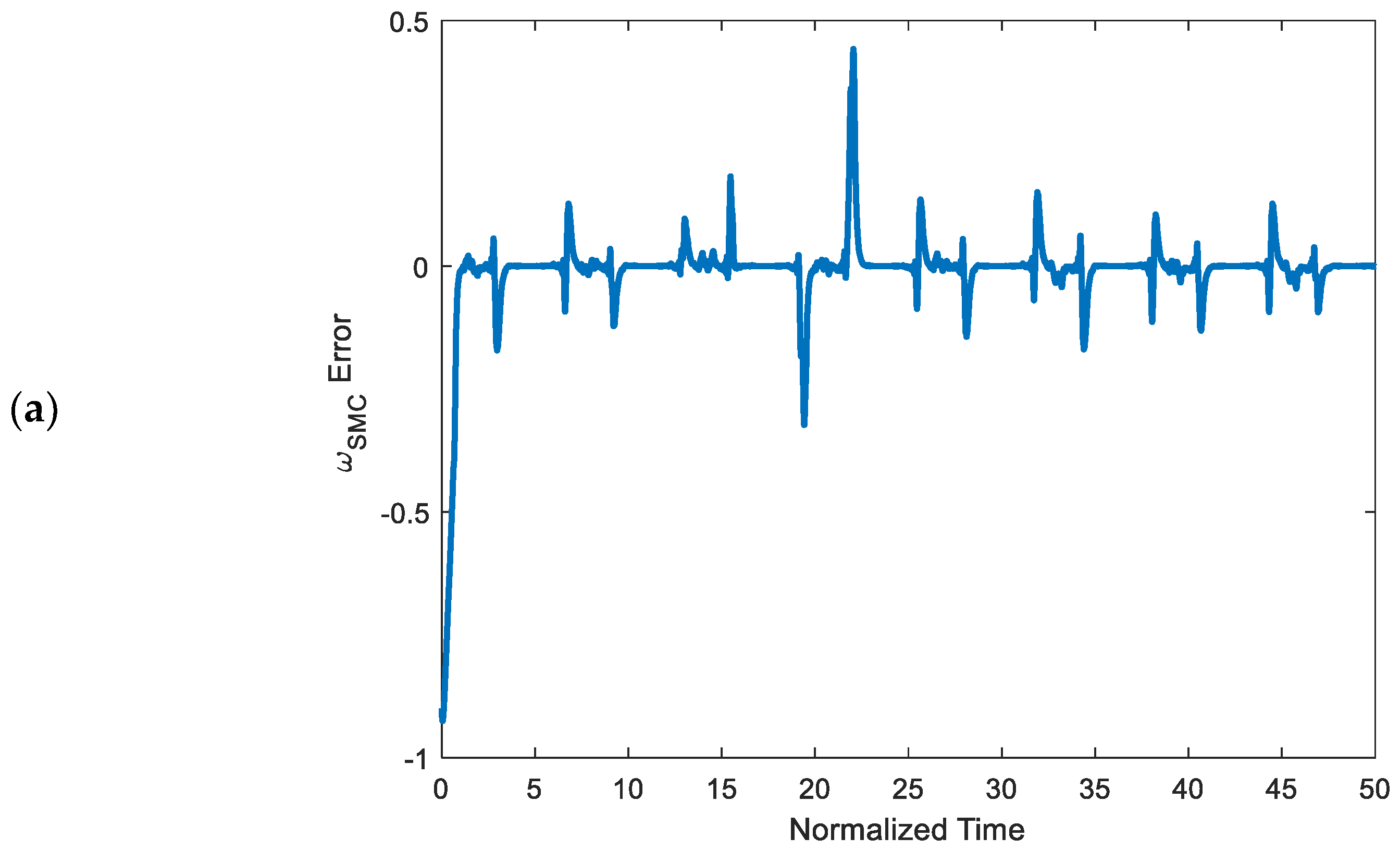
4.3. Robustness Test against Random Noise

HTGS is a complex system which is operating in a wide range of conditions; for this reason, it is arduous to model the system precisely. One of the critical factors of performance evaluation of a controller is its ability to seeking desire performance under uncertainties and external disturbances that impose on the system. In this part, the performance of SMC is compared with the proposed control method. During the simulation, the random noises that are imposed on the system are the same as [36]. The parameters of both controllers are kept unchanged in this simulation.

As it is shown in Figure 12 and Figure 13, when the HTGS is under random noises, the proposed controller has a smaller error amplitude and system rise time in comparison with SMC. Moreover, it is evident that the proposed control scheme has the acceptable ability to control the output of the system under random noises, and these noises could not have a noticeable influence on the performance of the proposed controller.

5. Conclusions

In this research, the dynamical behavior of a hydraulic generator regulating system was studied. Based on numerical tools such as phase diagrams, time series of the system with different initial conditions, and bifurcation diagram, dynamics of the system were investigated. It was illustrated that the maximum Lyapunov exponent is positive, which confirms the chaotic behavior of the given system. After that, a robust control method was proposed for the control of the HTGS in the presence of external disturbances and dynamic uncertainties. The ChNN was combined with a non-singular FTSMC in order to guarantee the appropriate performance of the controller in the presence of external disturbances and dynamic uncertainties. Finally, using numerical simulation, the performance of the proposed controller was investigated. Numerical results show the superiority of the proposed control strategy over the conventional sliding controller for the HTGS in terms of robustness and convergence time. It was demonstrated that although the dynamic of the systems is very complicated with high frequency, the ChNN estimates the unknown function of the system with proper accuracy (see Figure 9 and Figure 10), which confirmed the positive effects of the ChNN on the performance of the controller. It is noteworthy that the stability of the system under the proposed control method is limited to the case in which the time derivative of $W^{\ast }$ is approximately equal to zero. Hence, as a future work suggestion, some research can be conducted to use a deep reinforcement learning algorithm with the control scheme while the parameters of the system vary faster. Moreover, deep reinforcement learning algorithms can be applied in order to perform fault diagnostics of this system. Moreover, the presented ChNN-based non-singular fast terminal sliding mode method could be extended for fractional-order systems.

References

1. Qu, F.; Guo, W. Robust H control for hydro-turbine governing system of hydropower plant with super long headrace tunnel. Int. J. Electr. Power Energy Syst. 2020, 124, 106336. [Google Scholar] [CrossRef]
2. Li, R.; Arzaghi, E.; Abbassi, R.; Chen, D.; Li, C.; Li, H.; Xu, B. Dynamic maintenance planning of a hydro-turbine in operational life cycle. Reliab. Eng. Syst. Saf. 2020, 204, 107129. [Google Scholar] [CrossRef]
3. Xu, B.; Chen, D.; Tolo, S.; Patelli, E.; Jiang, Y. Model validation and stochastic stability of a hydro-turbine governing system under hydraulic excitations. Int. J. Electr. Power Energy Syst. 2018, 95, 156–165. [Google Scholar] [CrossRef] [Green Version]
4. Xu, B.; Chen, D.; Zhang, H.; Wang, F.; Zhang, X.; Wu, Y. Hamiltonian model and dynamic analyses for a hydro-turbine governing system with fractional item and time-lag. Commun. Nonlinear Sci. Numer. Simul. 2017, 47, 35–47. [Google Scholar] [CrossRef] [Green Version]
5. Yang, X.-J. A new integral transform operator for solving the heat-diffusion problem. Appl. Math. Lett. 2017, 64, 193–197. [Google Scholar] [CrossRef]
6. Yang, X.-J.; Abdel-Aty, M.; Cattani, C. A new general fractional-order derivataive with Rabotnov fractional-exponential kernel applied to model the anomalous heat transfer. Therm. Sci. 2019, 23, 1677–1681. [Google Scholar] [CrossRef] [Green Version]
7. Yu, X.; Yang, X.; Zhang, J. Stability analysis of hydro-turbine governing system including surge tanks under interconnected operation during small load disturbance. Renew. Energy 2018, 133, 1426–1435. [Google Scholar] [CrossRef]
8. Li, C.; Mao, Y.; Zhou, J.; Zhang, N.; An, X. Design of a fuzzy-PID controller for a nonlinear hydraulic turbine governing system by using a novel gravitational search algorithm based on Cauchy mutation and mass weighting. Appl. Soft Comput. 2017, 52, 290–305. [Google Scholar] [CrossRef]
9. Zeng, Y.; Zhang, L.; Guo, Y.; Qian, J.; Zhang, C. The generalized Hamiltonian model for the shafting transient analysis of the hydro turbine generating sets. Nonlinear Dyn. 2014, 76, 1921–1933. [Google Scholar] [CrossRef] [Green Version]
10. Trivedi, C.; Gandhi, B.K.; Cervantes, M.J.; Dahlhaug, O.G. Experimental investigations of a model Francis turbine during shutdown at synchronous speed. Renew. Energy 2015, 83, 828–836. [Google Scholar] [CrossRef]
11. Garcia, F.J.; Uemori, M.K.I.; Echeverria, J.J.R.; da Costa Bortoni, E. Design Requirements of Generators Applied to Low-Head Hydro Power Plants. IEEE Trans. Energy Convers. 2015, 30, 1630–1638. [Google Scholar] [CrossRef]
12. Jahanshahi, H.; Yousefpour, A.; Munoz-Pacheco, J.M.; Kacar, S.; Pham, V.-T.; Alsaadi, F.E. A new fractional-order hyperchaotic memristor oscillator: Dynamic analysis, robust adaptive synchronization, and its application to voice encryption. Appl. Math. Comput. 2020, 383, 125310. [Google Scholar] [CrossRef]
13. Iqbal, J.; Ullah, M.; Khan, S.G.; Khelifa, B.; Ćuković, S. Nonlinear Control Systems-A Brief Overview of Historical and Recent Advances. Nonlinear Eng. 2017, 6, 301–312. [Google Scholar] [CrossRef]
14. Jahanshahi, H.; Sari, N.N.; Pham, V.-T.; Alsaadi, F.E.; Hayat, T. Optimal adaptive higher order controllers subject to sliding modes for a carrier system. Int. J. Adv. Robot. Syst. 2018, 15. [Google Scholar] [CrossRef]
15. Jahanshahi, H.; Yousefpour, A.; Wei, Z.; Alcaraz, R.; Bekiros, S. A financial hyperchaotic system with coexisting attractors: Dynamic investigation, entropy analysis, control and synchronization. Chaos Solitons Fractals 2019, 126, 66–77. [Google Scholar] [CrossRef]
16. Jahanshahi, H.; Yousefpour, A.; Munoz-Pacheco, J.M.; Moroz, I.; Wei, Z.; Castillo, O. A new multi-stable fractional-order four-dimensional system with self-excited and hidden chaotic attractors: Dynamic analysis and adaptive synchronization using a novel fuzzy adaptive sliding mode control method. Appl. Soft Comput. 2019, 87, 105943. [Google Scholar] [CrossRef]
17. Yousefpour, A.; Vahidi-Moghaddam, A.; Rajaei, A.; Ayati, M. Stabilization of nonlinear vibrations of carbon nanotubes using observer-based terminal sliding mode control. Trans. Inst. Meas. Control. 2019, 42, 1047–1058. [Google Scholar] [CrossRef]
18. Yousefpour, A.; Jahanshahi, H.; Munoz-Pacheco, J.M.; Bekiros, S.; Wei, Z. A fractional-order hyper-chaotic economic system with transient chaos. Chaos Solitons Fractals 2019, 130, 109400. [Google Scholar] [CrossRef]
19. Asl, R.M.; Hagh, Y.S.; Palm, R. Robust control by adaptive Non-singular Terminal Sliding Mode. Eng. Appl. Artif. Intell. 2017, 59, 205–217. [Google Scholar] [CrossRef]
20. Yao, Q.; Jahanshahi, H.; Batrancea, L.M.; Alotaibi, N.D.; Rus, M.-I. Fixed-Time Output-Constrained Synchronization of Unknown Chaotic Financial Systems Using Neural Learning. Mathematics 2022, 10, 3682. [Google Scholar] [CrossRef]
21. Jahanshahi, H.; Yao, Q.; Khan, M.I.; Moroz, I. Unified neural output-constrained control for space manipulator using tan-type barrier Lyapunov function. Adv. Space Res. 2022, in press. [Google Scholar] [CrossRef]
22. Alsaade, F.W.; Yao, Q.; Bekiros, S.; Al-Zahrani, M.S.; Alzahrani, A.S.; Jahanshahi, H. Chaotic attitude synchronization and anti-synchronization of master-slave satellites using a robust fixed-time adaptive controller. Chaos Solitons Fractals 2022, 165, 112883. [Google Scholar] [CrossRef]
23. Yao, Q.; Jahanshahi, H.; Moroz, I.; Bekiros, S.; Alassafi, M.O. Indirect neural-based finite-time integral sliding mode control for trajectory tracking guidance of Mars entry vehicle. Adv. Space Res. 2022, in press. [Google Scholar] [CrossRef]
24. Lu, Y.-S. Sliding-Mode Disturbance Observer with Switching-Gain Adaptation and Its Application to Optical Disk Drives. IEEE Trans. Ind. Electron. 2009, 56, 3743–3750. [Google Scholar] [CrossRef]
25. Chen, M.; Chen, W.-H. Sliding mode control for a class of uncertain nonlinear system based on disturbance observer. Int. J. Adapt. Control Signal Process. 2009, 24, 51–64. [Google Scholar] [CrossRef]
26. Yousefpour, A.; Jahanshahi, H.; Castillo, O. Application of Variable-Order Fractional Calculus in Neural Networks: Where Do We Stand? Eur. Phys. J. Spec. Top. 2022, 231, 1–4. [Google Scholar] [CrossRef]
27. Li, Y.; Wei, X.; Li, Y.; Dong, Z.; Shahidehpour, M. Detection of False Data Injection Attacks in Smart Grid: A Secure Federated Deep Learning Approach. IEEE Trans. Smart Grid 2022, 13, 4862–4872. [Google Scholar] [CrossRef]
28. Xu, B.; Zhang, J.; Egusquiza, M.; Chen, D.; Li, F.; Behrens, P.; Egusquiza, E. A review of dynamic models and stability analysis for a hydro-turbine governing system. Renew. Sustain. Energy Rev. 2021, 144, 110880. [Google Scholar] [CrossRef]
29. Ding, X.; Sinha, A. Hydropower Plant Frequency Control Via Feedback Linearization and Sliding Mode Control. J. Dyn. Syst. Meas. Control 2016, 138, 074501. [Google Scholar] [CrossRef]
30. Ding, X.; Sinha, A. Hydropower Plant Load Frequency Control Via Second-Order Sliding Mode. J. Dyn. Syst. Meas. Control 2017, 139, 074503. [Google Scholar] [CrossRef]
31. Ling, D.J. Bifurcation and Chaos of Hydraulic Turbine Governor; Nanjing Hohai University: Nanjing, China, 2007. [Google Scholar]
32. Li, C.; Sprott, J.C.; Mei, Y. An infinite 2-D lattice of strange attractors. Nonlinear Dyn. 2017, 89, 2629–2639. [Google Scholar] [CrossRef]
33. Vyas, B.Y.; Das, B.; Maheshwari, R.P. Improved Fault Classification in Series Compensated Transmission Line: Comparative Evaluation of Chebyshev Neural Network Training Algorithms. IEEE Trans. Neural Netw. Learn. Syst. 2014, 27, 1631–1642. [Google Scholar] [CrossRef] [PubMed]
34. Chen, M.; Wu, Q.-X.; Cui, R. Terminal sliding mode tracking control for a class of SISO uncertain nonlinear systems. ISA Trans. 2012, 52, 198–206. [Google Scholar] [CrossRef]
35. The Math Works, Inc. MATLAB, Version 2020a; The Math Works, Inc.: Natick, MA, USA, 2020; Available online: Https://Www.Mathworks.Com/ (accessed on 28 May 2020).
36. Yuan, X.; Chen, Z.; Yuan, Y.; Huang, Y.; Li, X.; Li, W. Sliding mode controller of hydraulic generator regulating system based on the input/output feedback linearization method. Math. Comput. Simul. 2016, 119, 18–34. [Google Scholar] [CrossRef]
Figure 1. Phase diagrams of the system with increase initial value of δ 1 ( t 0 ) (a) t [ 0 ,     350 ] and (b) t [ 350 ,     500 ] .
Mathematics 11 00168 g001
Figure 2. Lyapunov exponents of system (1).
Mathematics 11 00168 g002
Figure 3. (a) Bifurcation diagram of the system with the variation of δ1(t0) and (b) the mean value of δ 1 .
Mathematics 11 00168 g003
Figure 4. The ChNN structure.
Mathematics 11 00168 g004
Figure 5. Scheme of ChNN-based non-singular FTSMC.
Mathematics 11 00168 g005
Figure 6. Step response of HTGS using (a) SMC and (b) proposed controller.
Mathematics 11 00168 g006
Figure 7. Position error of HTGS using (a) SMC and (b) proposed controller.
Mathematics 11 00168 g007
Figure 8. Periodic response of HTGS using (a) SMC and (b) proposed controller.
Mathematics 11 00168 g008
Figure 9. Position error of HTGS using (a) SMC and (b) proposed controller.
Mathematics 11 00168 g009aMathematics 11 00168 g009b
Figure 10. Output of the ChNN for step input.
Mathematics 11 00168 g010
Figure 11. Output of the neural network for periodic input.
Mathematics 11 00168 g011
Figure 12. Periodic response of HTGS under random noise (a) SMC and (b) proposed controller.
Mathematics 11 00168 g012
Figure 13. Periodic response of HTGS under random noise (a) SMC and (b) proposed controller.
Mathematics 11 00168 g013