Abstract
The intelligent driver (ID) model characterizes traffic behavior with a constant acceleration exponent and does not follow traffic physics. This results in unrealistic traffic behavior. In this paper, a new microscopic heterogeneous traffic flow model is proposed which improves the performance of the ID model. The forward and lateral distance headways are used to characterize traffic behavior. The stability of the ID and proposed models is examined over a 1000 m circular road with a traffic disturbance after 30 s. The results obtained show that the proposed model is more stable than the ID model. The performance of the proposed and ID models is evaluated over an 1800 m circular road for 150 s with a platoon of 51 vehicles. Results are presented which indicate that traffic evolves realistically with the proposed model. This is because it is based on the lateral distance headway.
1. Introduction
Urban traffic congestion is a major concern in developing countries [1]. Congestion causes traffic delays, excessive fuel consumption, pollution, and safety problems [2,3,4,5]. As urban populations increase, so does the number of vehicles [6]. In these areas, vehicles utilize vacant road space and lane discipline is often ignored, resulting in heterogeneous traffic [7]. The distance covered by a vehicle to align to forward vehicles in a lane is known as the forward distance headway, and the lateral distance between vehicles is called the lateral distance headway. These headways affect driver response and cause traffic flow variations [8]. Vehicles in heterogeneous traffic adjust their position and speed based on the lateral distance headway. Thus, the realistic characterization of heterogeneous traffic requires a model that considers this headway and lane-changing behavior.
Three types of models are employed for traffic flow characterization: microscopic, macroscopic, and mesoscopic. Microscopic models consider individual vehicle behavior and are often based on driver physical and psychological responses [9]. These models employ parameters such as vehicle position, velocity, and time and distance headways [10]. They are used to predict vehicle dynamics [6]. Macroscopic models consider aggregate vehicle behavior [11], whereas mesoscopic models take into account both individual and aggregate behavior [12].
Gazis et al. [13] developed a microscopic model which considers driver response to forward traffic conditions based on the velocity difference. Drivers adjust their speed with a constant delay of s, so driver behavior due to traffic conditions is ignored. Newell [14] proposed a model for vehicle behavior in dense traffic. Velocity is based on the distance headway, so a larger distance headway results in a lower density and, hence, a greater velocity. However, this relationship results in high acceleration, which is not realistic [15]. Moreover, this model neglects variations in driver behavior as a constant time headway is employed [16].
Bando et al. [17] improved the Newell model but neglected velocity differences resulting in unstable behavior. Moreover, deviations from the equilibrium velocity result in high acceleration, which is not realistic. Further, small distances between vehicles occur, which can result in accidents. Helbing and Tilch [18] developed a model which considers the reaction to velocity differences and, thus, accurately characterizes the time headway and velocity during congestion. However, acceleration occurs over a short time, which is typical of an aggressive driver, so slow and average driver behavior is neglected. Gipps [19] proposed a model based on driver response to forward traffic with realistic acceleration. However, this model is only suitable for a small range of parameters.
Treiber, Henneck, and Helbing [15] developed the intelligent driver (ID) model based on driver response. With this model, driver behavior is based on the velocity and distance headway of forward vehicles, and typical traffic parameters are employed [20,21,22]. However, the acceleration exponent, , in the ID model is a constant and so cannot characterize driver behavior under different traffic conditions. To improve the ID model for intersections, driver response based on deceleration has been incorporated [23]. However, the distance between vehicles is small at high velocities, which can result in accidents. This distance can be adjusted using parameters based on velocity [24]. The ID model has been used to characterize connected and autonomous vehicles (CAVs) [25,26]. However, this model does not provide realistic CAV behavior for real traffic conditions [27].
A model integrating psychoticism, extraversion, and neuroticism (PEN) was proposed in [28] for heterogeneous traffic. However, this model ignores traffic physics, so the results can be unrealistic. A microscopic car-following model for CAVs in heterogeneous traffic was proposed in [29] to mitigate oscillations and improve traffic flow. However, this model is complex and so is difficult to implement. A traffic model based on distance headway was developed in [30], but a constant lateral distance headway is used, which is unrealistic [7].
Gunay [31] proposed a model which characterizes non-lane-based traffic considering the positions of leading vehicles. However, heterogeneous traffic and lane discipline are ignored [32]. In heterogeneous traffic, vehicles interact both longitudinally and laterally and are strongly correlated [7]. Moreover, the road capacity is higher with heterogeneous traffic due to the gap-filling behavior [33] as shown in Figure 1. Lane changes increase acceleration and deceleration and can result in stop-and-go traffic behavior [34] and increase the probability of accidents [35].

Figure 1.
(a) Lane-based homogenous traffic. (b) Non-lane-based heterogeneous traffic with gap-filling behavior.
In this paper, a new microscopic heterogeneous traffic model is proposed which characterizes traffic behavior based on the forward and lateral distance headways. The performance of the ID and proposed models is evaluated over an m circular road for s, and the stability is examined over a m circular road for s. A shorter duration is used for the stability analysis as this is sufficient to evaluate model behavior. The results obtained indicate that traffic behavior with the proposed model is more realistic.
2. Traffic Flow Models
The ID model is a microscopic model that presumes forward traffic conditions [36]. It characterizes acceleration based on driver response, the distance between vehicles, and the time required to align to forward vehicles. According to this model, driver response is based on the ratio of average velocity to maximum velocity. Acceleration depends on this ratio and traffic flow is smooth when this ratio is .
The ID model acceleration is given by [15]:
where is the maximum acceleration, is the maximum velocity, is the average velocity, and is the bumper-to-bumper distance between vehicles. is the distance headway covered during traffic alignment, which can be expressed as [15]:
where is the traffic jam spacing, is the time headway, is the maximum acceleration, and is the difference in velocity between the following and leading vehicles.
The ID model characterizes driver response based on an acceleration exponent, , which is a constant. This constant must represent driver behavior for a variety of traffic conditions. However, it does not follow traffic flow physics and, thus, can result in unrealistic behavior. Therefore, an acceleration exponent based on heterogeneous traffic is proposed to better characterize traffic.
In heterogeneous traffic, driver response is based on the forward and lateral distance headways as well as lane-changing behavior and is given by:
where is the difference in velocity between the following and leading vehicles, which characterizes lane changes and traffic alignment during these changes. is the traffic density, is the distance headway between the following and leading vehicles as shown in Figure 2, and is the lateral distance headway. A driver reacts to perceived conditions and aligns with the forward and adjacent vehicles. The reaction is quick for a small distance headway as alignment occurs over a short distance and vice versa for a longer distance headway. In other words, vehicle movement is greater with a larger distance headway.
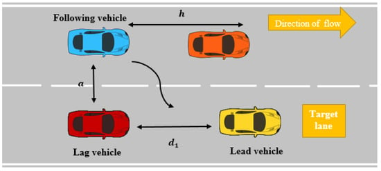
Figure 2.
Heterogeneous traffic with lane changing.
In heterogeneous traffic, the lateral distance headway varies and is small during congestion. Further, when the traffic density is large, the forward distance headway, , is small, so:
Substituting (4) in (3) we have:
and replacing in (1) with this expression gives the proposed model:
This model characterizes heterogeneous traffic based on the forward and lateral distance headways. It is better than the ID model because it is based on traffic conditions rather than on a number, which is a compromise to fit all conditions.
For microscopic models, traffic density is given by [37] where is the distance headway at equilibrium. At equilibrium, , so from (2):
For the proposed model, the equilibrium distance headway is:
Equation (7) shows that the equilibrium distance headway for the ID model is based on a constant exponent which is the same for all traffic conditions. Conversely, this headway for the proposed model (8) is based on heterogeneous traffic parameters and is not a constant.
Traffic flow is the product of velocity and density, [20], so the flow for the ID model is:
Substituting the proposed acceleration exponent term, the traffic flow for the proposed model is:
This flow is based on heterogeneous traffic parameters and so is more realistic than the flow for the ID model.
3. Stability Analysis
The stability of the ID and proposed models is evaluated over a m circular road for s. The value of the acceleration exponent ranges from to and is typically [15]. Typical values of the lateral distance headway are in the range of m to m [38]. Hence, the ID model is evaluated for , and and the proposed model for , and m. The leading vehicle velocity is m/s and the following vehicle velocity is 30 m/s, so m/s. The distance headway, , varies between m and m [39], and here it is set to m. The initial equilibrium velocity is m/s and the number of vehicles on the road is . The disturbance is induced at s at the maximum acceleration of 1.67 m/s2. The stability analysis parameters are given in Table 1.

Table 1.
Stability analysis parameters.
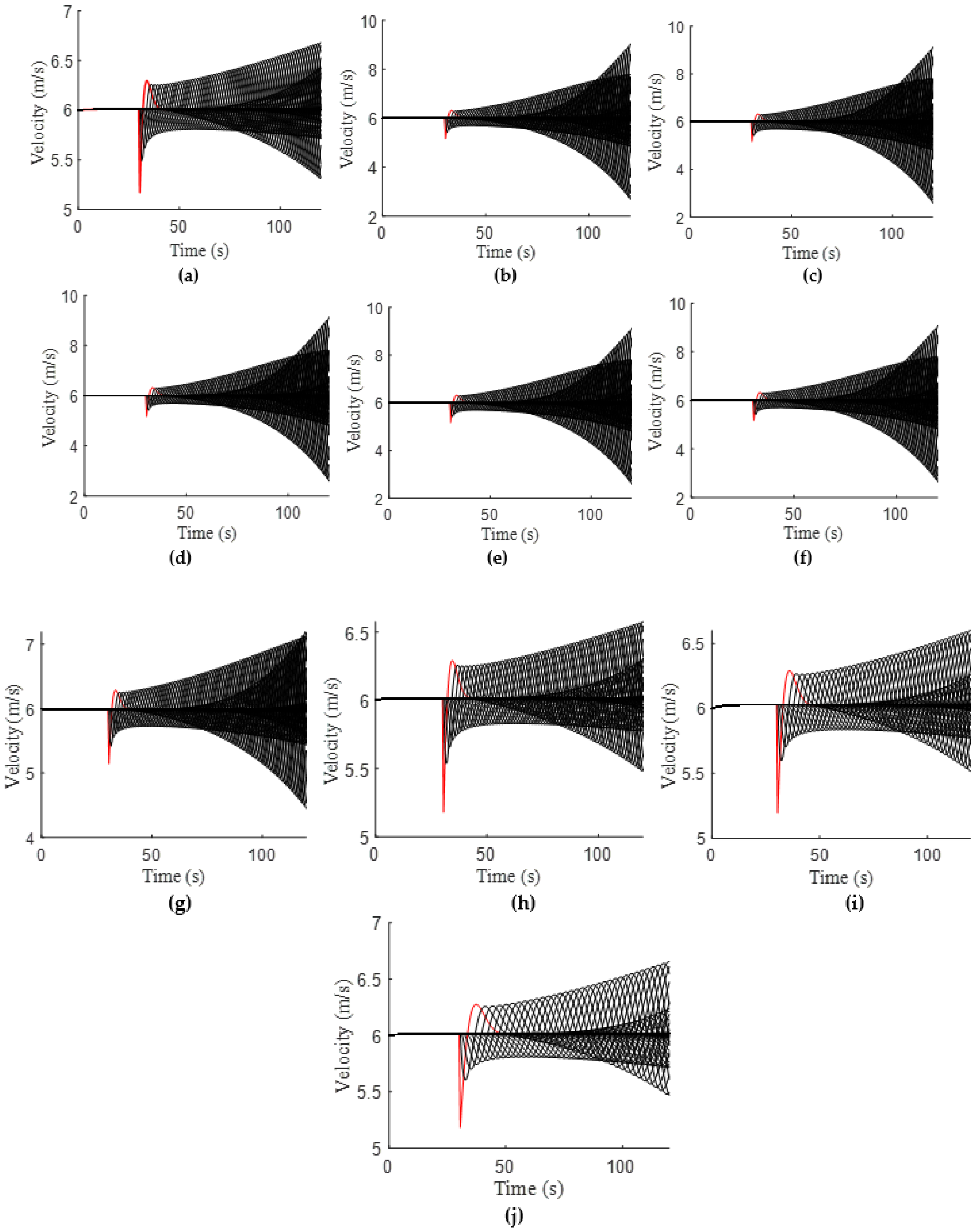
The velocity evolution of the ID and proposed models is given in Figure 3. The red line is the trajectory of the st vehicle and the black lines are the trajectories of the following vehicles. For the ID model, with , the velocity of the 1st vehicle suddenly drops to m/s at s and then increases to m/s at s and starts to oscillate. At s, the velocity oscillates between m/s and m/s, and at s, the velocity oscillates between m/s and m/s, as shown in Figure 3a. With , the velocity of the 1st vehicle suddenly drops to m/s at s and then increases to m/s at s and starts to oscillate. At s, the velocity oscillates between m/s and m/s, and at s, it oscillates between m/s and m/s, as shown in Figure 3b. With , the velocity of the 1st vehicle suddenly drops to m/s at s and then increases to m/s at s and starts to oscillate. At s, the velocity oscillates between m/s and m/s, and at s, the velocity oscillates between m/s and m/s, as shown in Figure 3c. With , the velocity of the 1st vehicle suddenly drops to m/s at s and then increases to m/s at s and starts to oscillate. At s, the velocity oscillates between m/s and m/s, and at s, the velocity oscillates between m/s and m/s, as shown in Figure 3d.
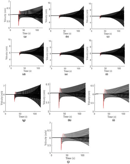
Figure 3.
Velocity evolution of the ID and proposed models with an initial equilibrium velocity of m/s: (a) ; (b) ; (c) ; (d) ; (e) m; (f) m; (g) m; (h) m; (i) m; (j) m.
For the proposed model, with m, the velocity of the 1st vehicle suddenly drops to m/s at s and then increases to m/s at s and starts to oscillate. At s, the velocity oscillates between m/s and m/s, and at s, the velocity oscillates between m/s and m/s, as shown in Figure 3e. With m, the velocity of the 1st vehicle suddenly drops to m/s at s and then increases to m/s at s and starts to oscillate. At s, the velocity oscillates between m/s and m/s, and at s, the velocity oscillates between m/s and m/s, as shown in Figure 3f. With m, the velocity of the 1st vehicle suddenly drops to m/s at s and then increases to m/s at s and starts to oscillate. At s, the velocity oscillates between m/s and m/s, and at s, the velocity oscillates between m/s and m/s, as shown in Figure 3g. With m, the velocity of the 1st vehicle suddenly drops to m/s at s and then increases to m/s at s and starts to oscillate. At s, the velocity oscillates between m/s and m/s, and at s, the velocity oscillates between m/s and m/s, as shown in Figure 3h. With m, the velocity of the 1st vehicle suddenly drops to m/s at s and then increases to m/s at s and starts to oscillate. At s, the velocity oscillates between m/s and m/s, and at s, the velocity oscillates between m/s and m/s, as shown in Figure 3i. With m, the velocity of the 1st vehicle suddenly drops to m/s at s and then increases to m/s at s and starts to oscillate. At s, the velocity oscillates between m/s and m/s, and at s, the velocity oscillates between m/s and m/s, as shown in Figure 3j.
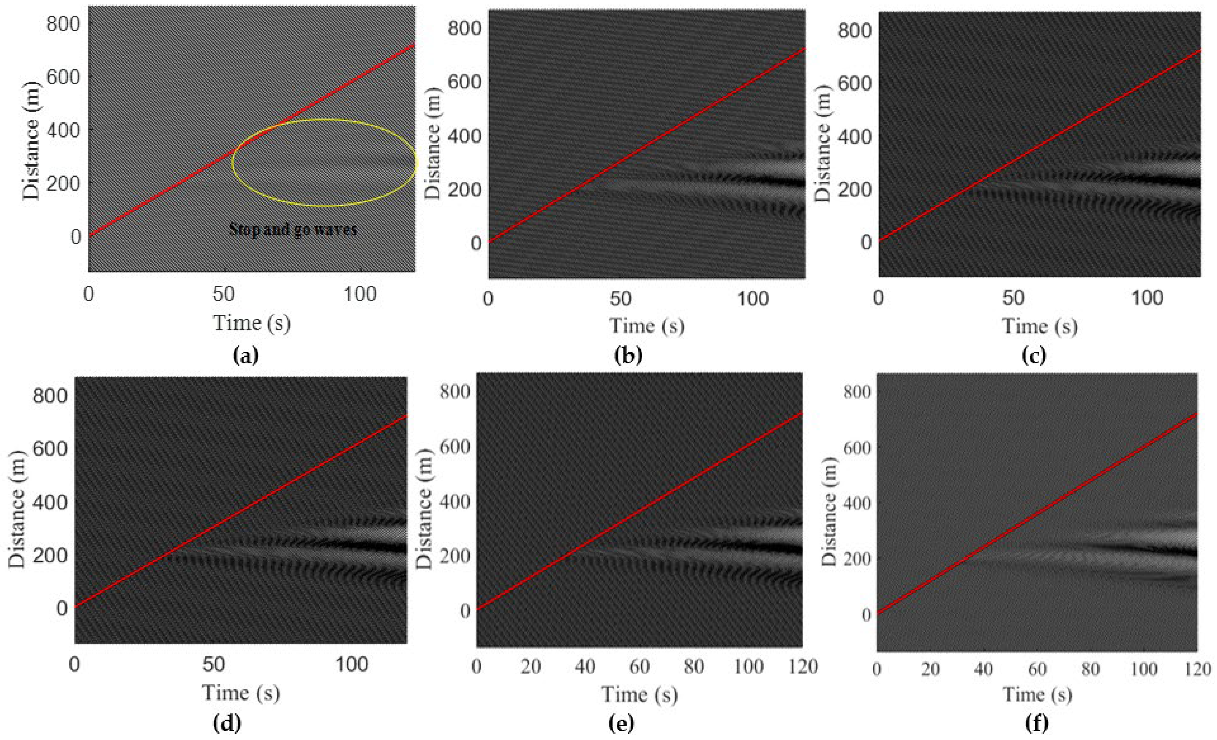
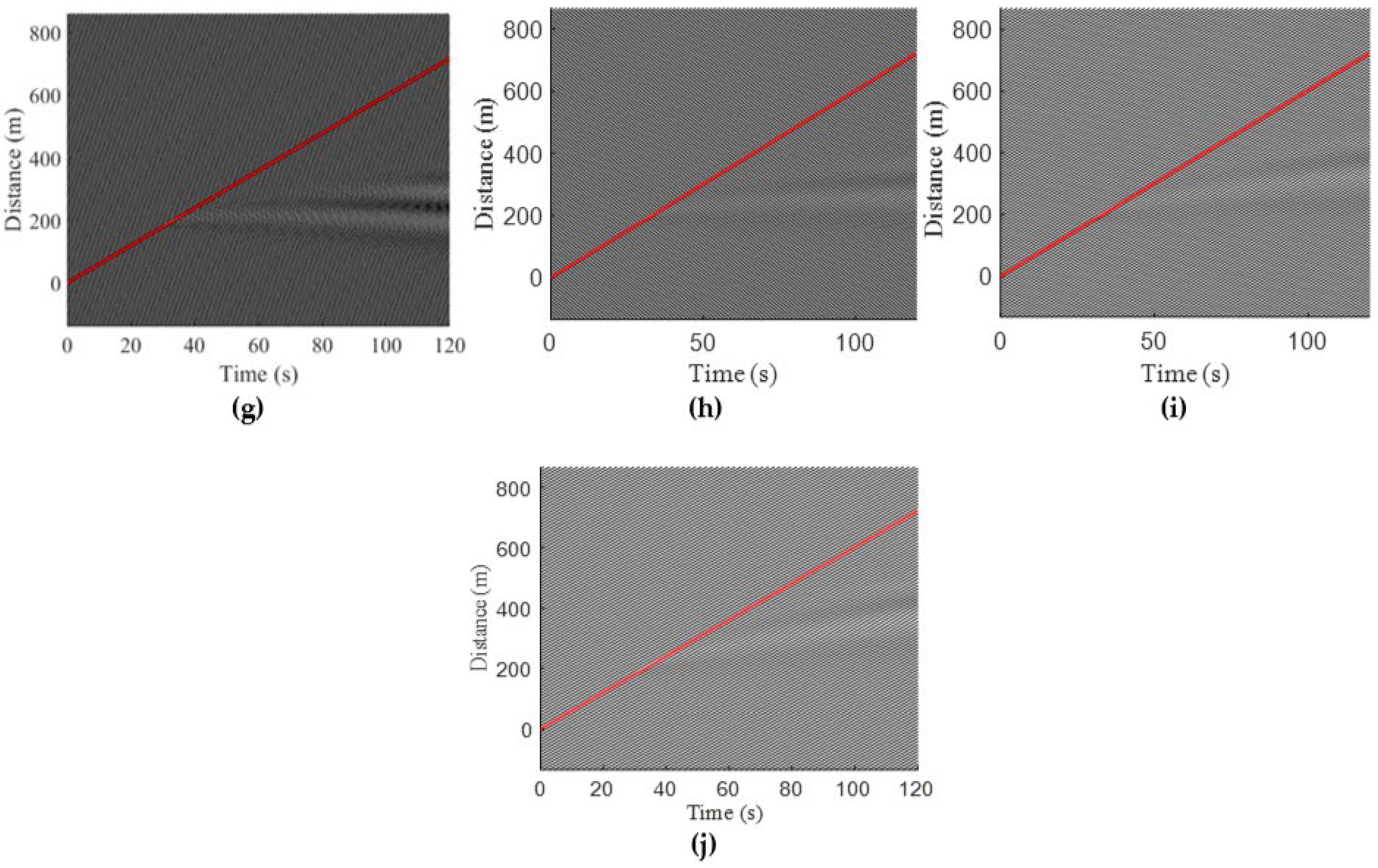
The time and space evolution of the vehicles for the ID and proposed models is given in Figure 4. This shows vehicle mobility and stop-and-go behavior due to congestion. Both models produce stop-and-go waves after a few seconds. For the ID model, from to , an increase in increases the stop-and-go waves produced over time and space, and above , the behavior is similar to that for , as shown in Figure 4a–d. Conversely, for the proposed model, the stop-and-go waves produced decrease as the lateral distance headway increases.
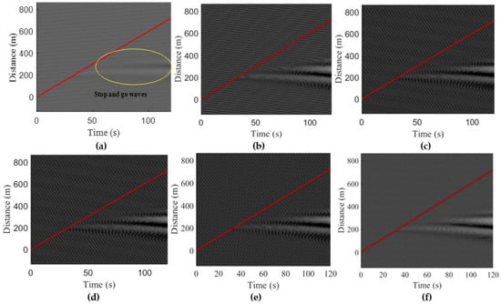
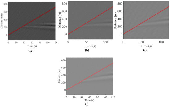
Figure 4.
Spatio-temporal performance of the ID and proposed models over a m circular road: (a) ; (b) ; (c) ; (d) ; (e) m; (f) m; (g) m; (h) m; (i) m; (j) m.
These results show that with the ID model, as increases from 1 to 10, the velocity oscillations increase as indicated in Figure 3a–c, but above , these oscillations are similar. This unstable and unrealistic behavior occurs because of the constant exponent. With the proposed model, as the lateral distance headway increases the velocity oscillations decrease over time. This behavior is more stable and realistic than the ID model because the proposed model is based on real traffic parameters. Furthermore, with the proposed model, the traffic is smooth as the stop-and-go waves produced are based on the lateral distance headway and decrease with an increase in this headway, as shown in Figure 4.
4. Performance Results
In this section, the performance of the proposed and ID models is evaluated over a circular road of length m for s using the Euler technique with a time step of s [37]. The simulation parameters are given in Table 2. The forward distance headway is m [40]. The lateral distance headway is typically between m and m [38], so here and m are used. The difference in velocity for the proposed model is m/s. The distance headway, , typically varies between m and m [39], so here it is set to m. The acceleration exponent ranges from to and is typically [15], so here and are used. The maximum normalized density at m/s is . There are 51 vehicles on the road which was obtained by dividing the road length by .

Table 2.
Simulation parameters.
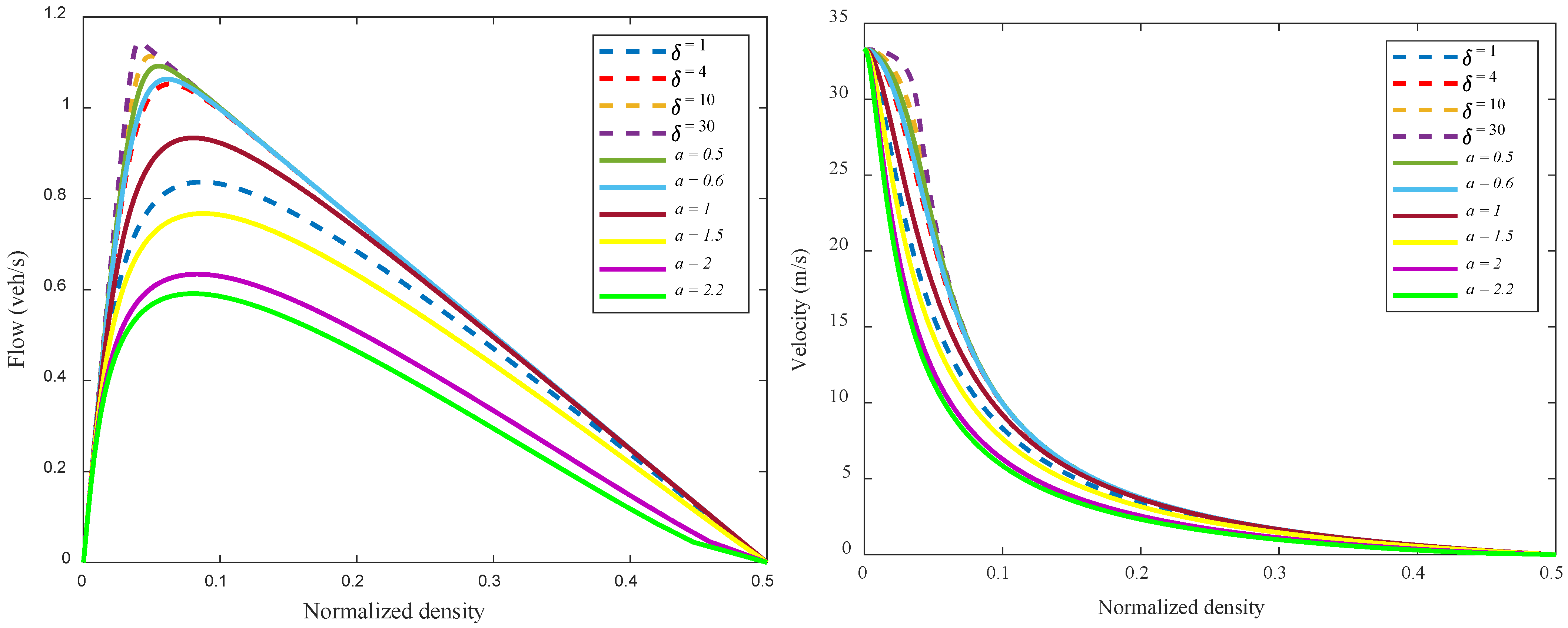
Figure 5 presents the flow and velocity behavior of the ID and proposed models. The results are summarized in Table 3 and Table 4. For the ID model, with the maximum flow is veh/s at density , and the corresponding critical velocity is m/s. With , the maximum flow is veh/s at density , and the critical velocity is m/s. With and , the maximum flow is veh/s and veh/s, respectively, at density , and the critical velocity is m/s. Table 3 shows that as increases, the maximum flow also increases, and the maximum density between and decreases with and is similar for values above . The critical velocity between and increases with whereas above , it is similar.
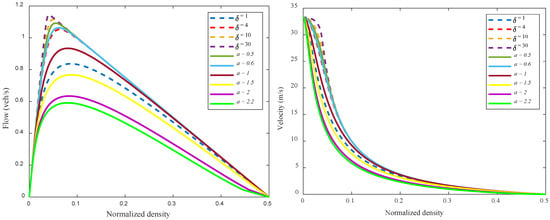
Figure 5.
Flow and velocity of the ID and proposed models.

Table 3.
Maximum flow, density, and critical velocity for the ID model.

Table 4.
Maximum flow, density, and critical velocity for the proposed model.
For the proposed model, with m, the maximum flow is veh/s at density , and the critical velocity is m/s. With m and m, the maximum flow is veh/s and veh/s at densities and respectively. The corresponding critical velocities are m/s and m/s, respectively. With m and m, the maximum flow is veh/s and veh/s at densities and , respectively. The corresponding critical velocities are m/s and m/s, respectively. With m, the maximum flow is veh/s at density and the critical velocity is m/s. Table 4 shows that as the lateral distance headway increases, the maximum flow decreases, and the maximum density increases between and m but decreases above . The critical velocity decreases between and m but increases for m.
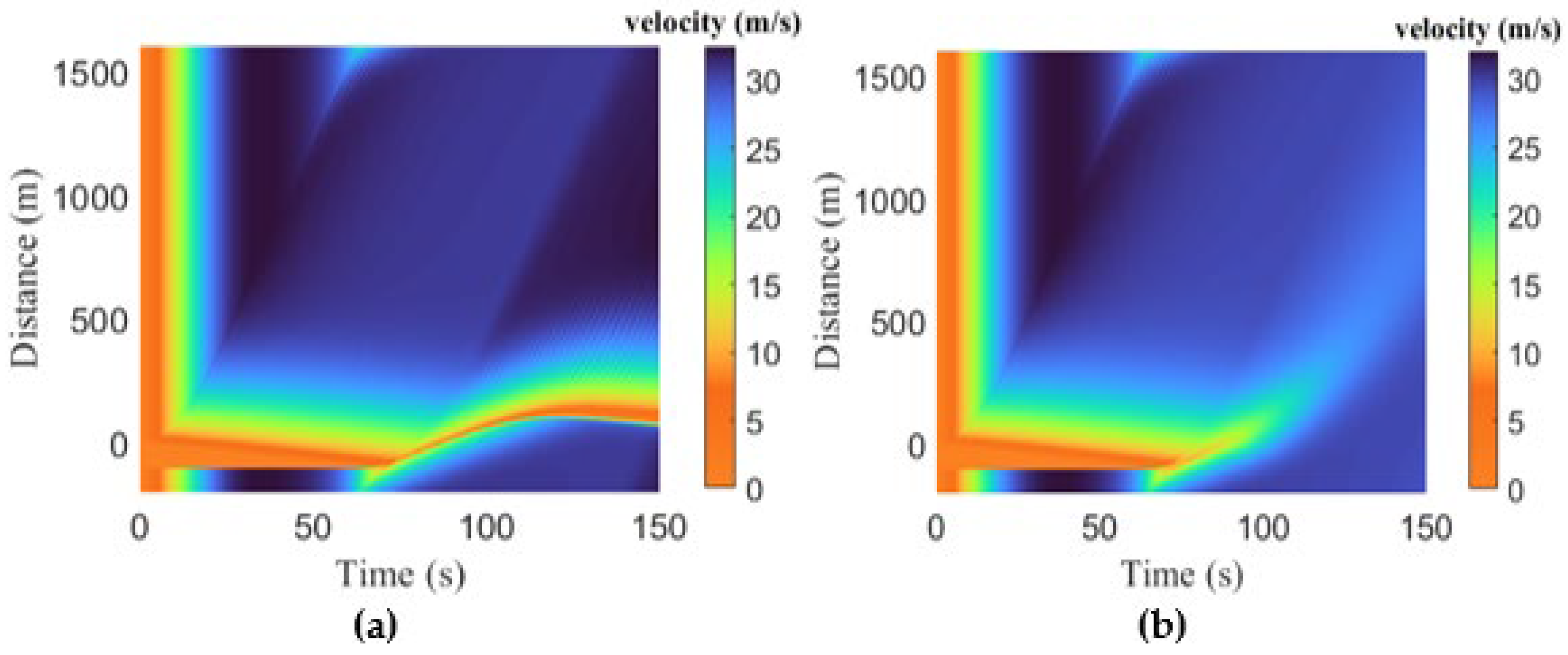
The spatio–temporal evolution of the queue caused due to congestion for the ID model is given in Figure 6, and the results are summarized in Table 5. This shows that the velocity during the queue is zero. For the ID model with , the queue dissolves at s, as shown in Figure 6a, and the velocity after the queue is m/s at s. With , the queue dissolves at s, as shown in Figure 6b, and the velocity after the queue is m/s at s. With = 10 and , the queue occurs between s and s. The velocity after the queue dissolves is m/s at s, and gradually decreases to m/s at s. The queue develops again at s and lasts until s between m and m, as shown in Figure 6c,d. For between and , the maximum velocity increases with but above , it is similar, as shown in Figure 6a–d.
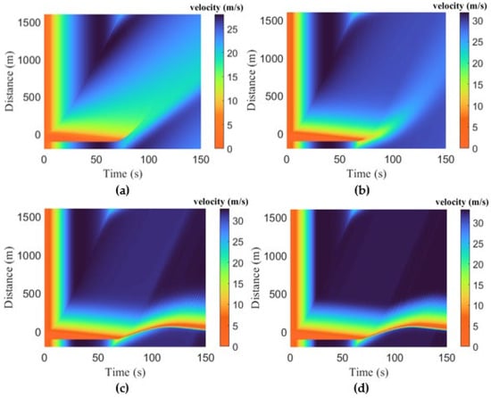
Figure 6.
Velocity evolution over time and space for the ID model on an m circular road: (a) ; (b) ; (c) ; (d) .

Table 5.
Velocity and time for the ID model during and after congestion.
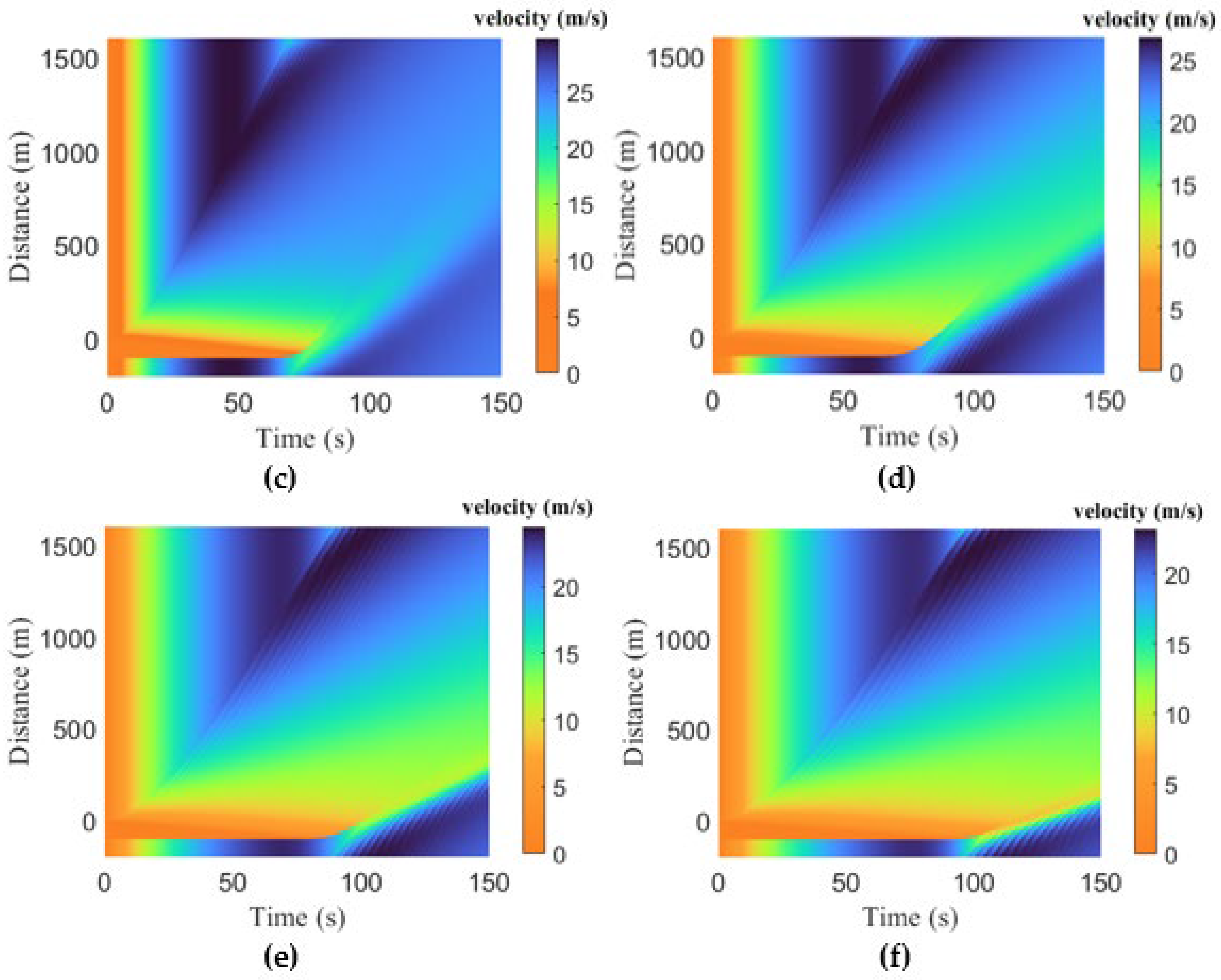
The spatio–temporal evolution of the queue due to congestion for the proposed model is given in Figure 7 and the results are summarized in Table 6. This shows that the velocity during the queue is zero. For the proposed model, with m, the queue exists between s and s. The velocity after the queue dissolves varies between m/s at s and m/s at s. The queue develops again at s and lasts until s between m and m, as shown in Figure 7a. With m and m, the queue dissolves at s and s, respectively, as shown in Figure 7b,c. The velocity after the queue dissolves with m is m/s and with m is m/s at s and s, respectively. With m and m, the queue dissolves at s and s, respectively, as shown in Figure 7d,e. The velocity after the queue dissolves with m is m/s and with m is m/s at s and s, respectively. With m, the queue dissolves at s, as shown in Figure 7f, and the velocity after the queue is m/s at s. Figure 7a–f indicate that as the lateral distance headway increases, the maximum velocity decreases.

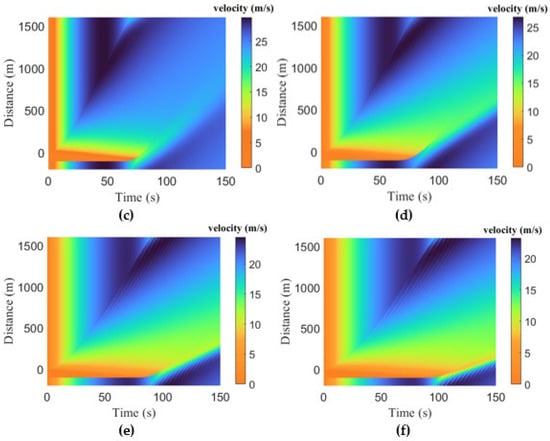
Figure 7.
Velocity evolution over time and space for the proposed model on an m circular road: (a) m; (b) m; (c) m; (d) m; (e) m; (f) m.

Table 6.
Velocity and time for the proposed model during and after congestion.
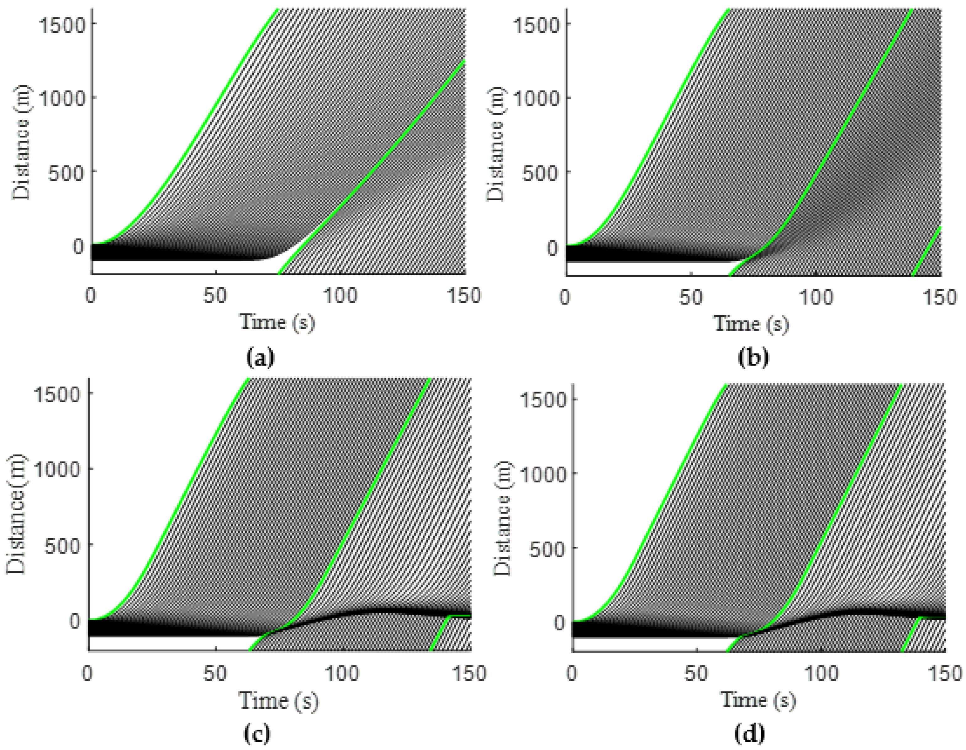
Figure 8 presents the time and space vehicle trajectories of a platoon of vehicles over an circular road for the ID model. The initial average velocity of the platoon is m/s. The green trajectory is the st vehicle that begins to move at s, whereas the black trajectories are of the following vehicles. With and , the traffic queue appears for s, as shown in Figure 8a,b, i.e., the st vehicle is in the queue for s. With , the initial queue appears for s. The st vehicle is in the queue for s at m and the last vehicle is in the queue for s at m. The queue appears again at s and lasts until s between m and m, respectively, as shown in Figure 8c. With , the initial queue appears for s. The st vehicle is in the queue for s at m and the last vehicle is in the queue for s at m. The queue appears again at s and lasts until s between m and m, respectively, as shown in Figure 8d.
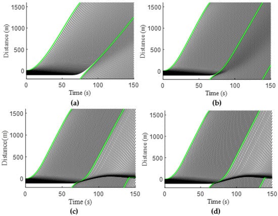
Figure 8.
Time–space vehicle trajectories for the ID model over an m circular road: (a) ; (b) ; (c) ; (d) . The colored line shows the trajectory of the first vehicle.
The positions of the 1st, 30th, and 40th vehicles at s are given in Table 7. With , the position of the 1st vehicle is m, whereas the positions of the 30th and 40th vehicles are m and m, respectively. With , the position of the 1st vehicle is m, whereas the positions of the 30th and 40th vehicles are m and m, respectively. With , the position of the 1st vehicle is m, whereas the positions of the 30th and 40th vehicles are m and m, respectively. With , the position of the 1st vehicle is m, whereas the positions of the 30th and 40th vehicles are m and m, respectively. Table 7 indicates that as increases, the distance traveled by the st vehicle increases. The distance traveled by the th and th vehicles decreases between and , and increases between and . Above , the distance traveled again decreases.

Table 7.
Position of the st, th, and th vehicles at s for the ID model.
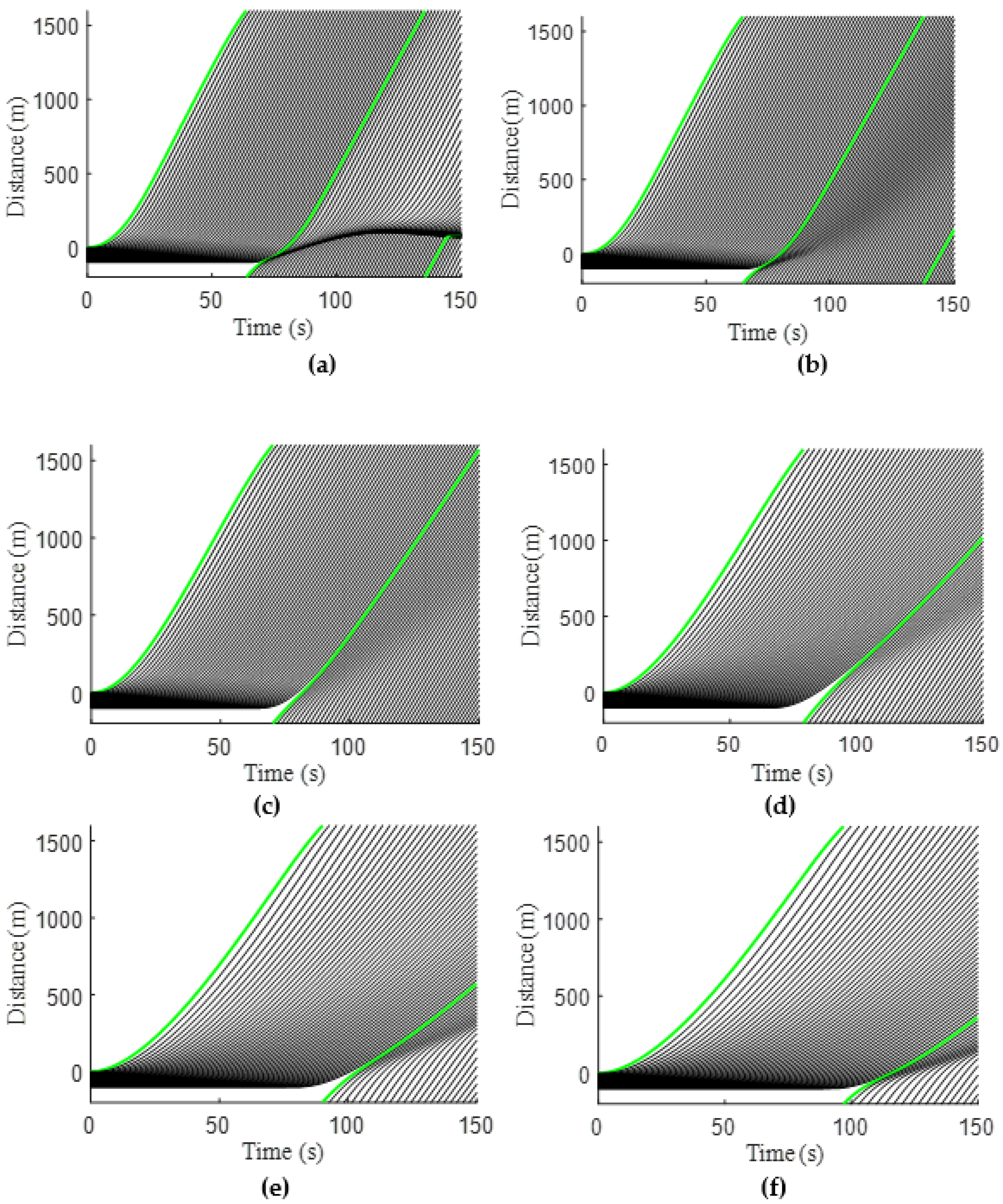
Figure 9 presents the time and space vehicle trajectories for the proposed model. With m, the initial queue appears for s. The st vehicle is in the queue for s at m and the last vehicle is in the queue for s at m. The queue appears again at s and lasts until s between m and m, respectively, as shown in Figure 9a. With and m, the queue appears for s and s, respectively, as shown in Figure 9b,c, so the st vehicle is in the queue for at m and s at m. With and m, the queue appears for s and s, respectively, as shown in Figure 9d,e, so the st vehicle is in the queue for s at m and s at m. With m, the queue appears for s, as shown in Figure 9f, so the st vehicle is in the queue for s at m.
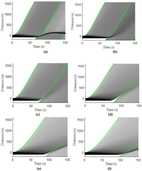
Figure 9.
Time–space vehicle trajectories for the proposed model over an m circular road: (a) m; (b) m; (c) m; (d) m; (e) m; (f) m. The colored line shows the trajectory of the first vehicle.
The positions of the 1st, 30th, and 40th vehicles at s are given in Table 8. With m, the position of the 1st vehicle is m, whereas the positions of the 30th and 40th vehicles are m and m, respectively. With m, the position of the 1st vehicle is m, whereas the positions of the 30th and 40th vehicles are m and m, respectively. With m, the position of the 1st vehicle is m, whereas the positions of the 30th and 40th vehicles are m and m, respectively. With m, the position of the 1st vehicle is m, whereas the positions of the 30th and 40th vehicles are m and m, respectively. With m, the position of the 1st vehicle is m, whereas the positions of the 30th and 40th vehicles are m and m, respectively. With m, the position of the 1st vehicle is m, whereas the positions of the 30th and 40th vehicles are m and m, respectively. Table 8 indicates that as increases, the distance traveled by the st and th vehicles decreases. The distance traveled by the th vehicle increases between m and m but decreases between m and m.

Table 8.
Positions of the st, th, and th vehicles at s for the proposed model.
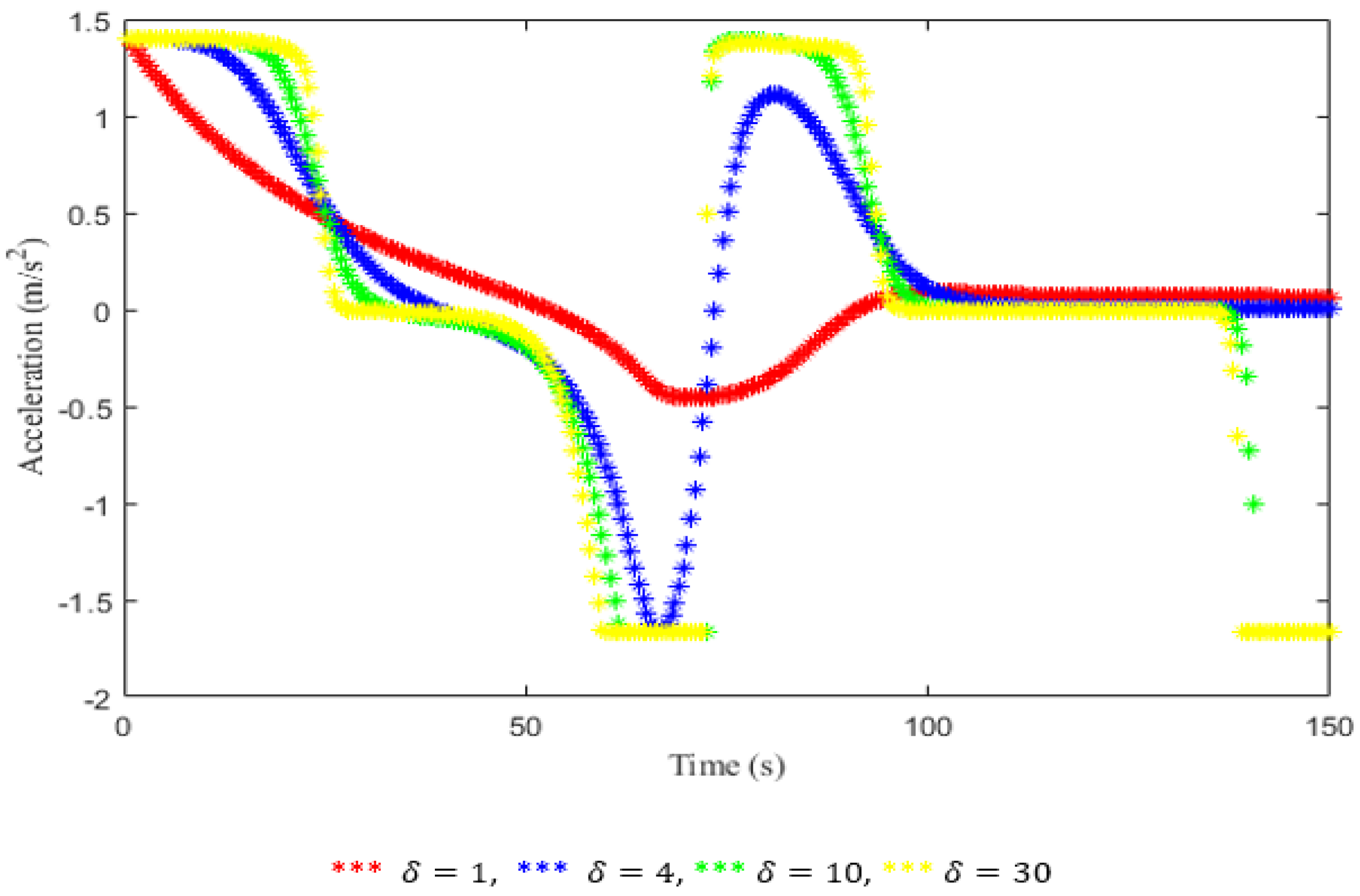
The temporal evolution of the acceleration for the ID model with and is given in Figure 10. With the acceleration at s is m/s2. It then decreases to m/s2 at s and increases to m/s2 at s. It decreases to m/s2 at s and is approximately constant until s. With , the acceleration at s is m/s2. It then decreases to m/s2 at s and m/s2 at s. It increases to m/s2 at s and decreases to m/s2 at s, and is approximately constant until s. With , the acceleration at s is m/s2. It then decreases to m/s2 at s and m/s2 at s, and is approximately constant until s. It increases to m/s2 between s and s and decreases to m/s2 between and s. It decreases to m/s2 at s and is approximately constant until s. With , the acceleration at s is m/s2. It then decreases to m/s2 at s and m/s2 at s, and is approximately constant until s. It increases to m/s2 between s and s and decreases to m/s2 between s and s. It then decreases to m/s2 at s and is approximately constant until s.

Figure 10.
Temporal evolution of acceleration for the ID model.
The temporal evolution of acceleration for the proposed model with and m is given in Figure 11. With m, the acceleration at s is m/s2. It then decreases to m/s2 at s and m/s2 at s, and is approximately constant until s. It increases to m/s2 at s and decreases to m/s2 at s and m/s2 at s. It then decreases to m/s2 at s and is approximately constant until s. With m, the acceleration at s is m/s2. It then decreases to m/s2 at s and m/s2 at s, and then it is approximately constant until s. It increases to m/s2 at s and decreases to m/s2 at s and m/s2 at s. With m, the acceleration at s is m/s2. It then decreases to m/s2 at s and m/s2 at s. It increases to m/s2 at s and then decreases to m/s2 at s and m/s2 at s, and is approximately constant until s. With m, the acceleration at s is m/s2. It then decreases to m/s2 at s and m/s2 at 68.5 s. It decreases to m/s2 at s and increases to m/s2 at s and m/s2 at s, and is approximately constant until s. With m, the acceleration at s is m/s2. It then decreases to m/s2 at s and m/s2 at s. It decreases to m/s2 at s and increases to m/s2 at s. It then decreases again to m/s2 at s and is approximately constant until s. With m, the acceleration at s is m/s2. It then decreases to m/s2 at s and m/s2 at s. It decreases to m/s2 at s, increases to m/s2 at s, and then decreases to m/s2 at s.
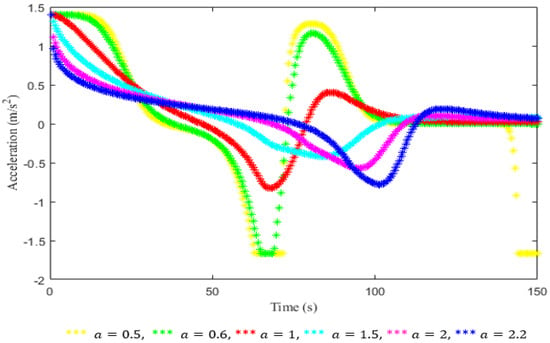
Figure 11.
Temporal evolution of acceleration for the proposed model.
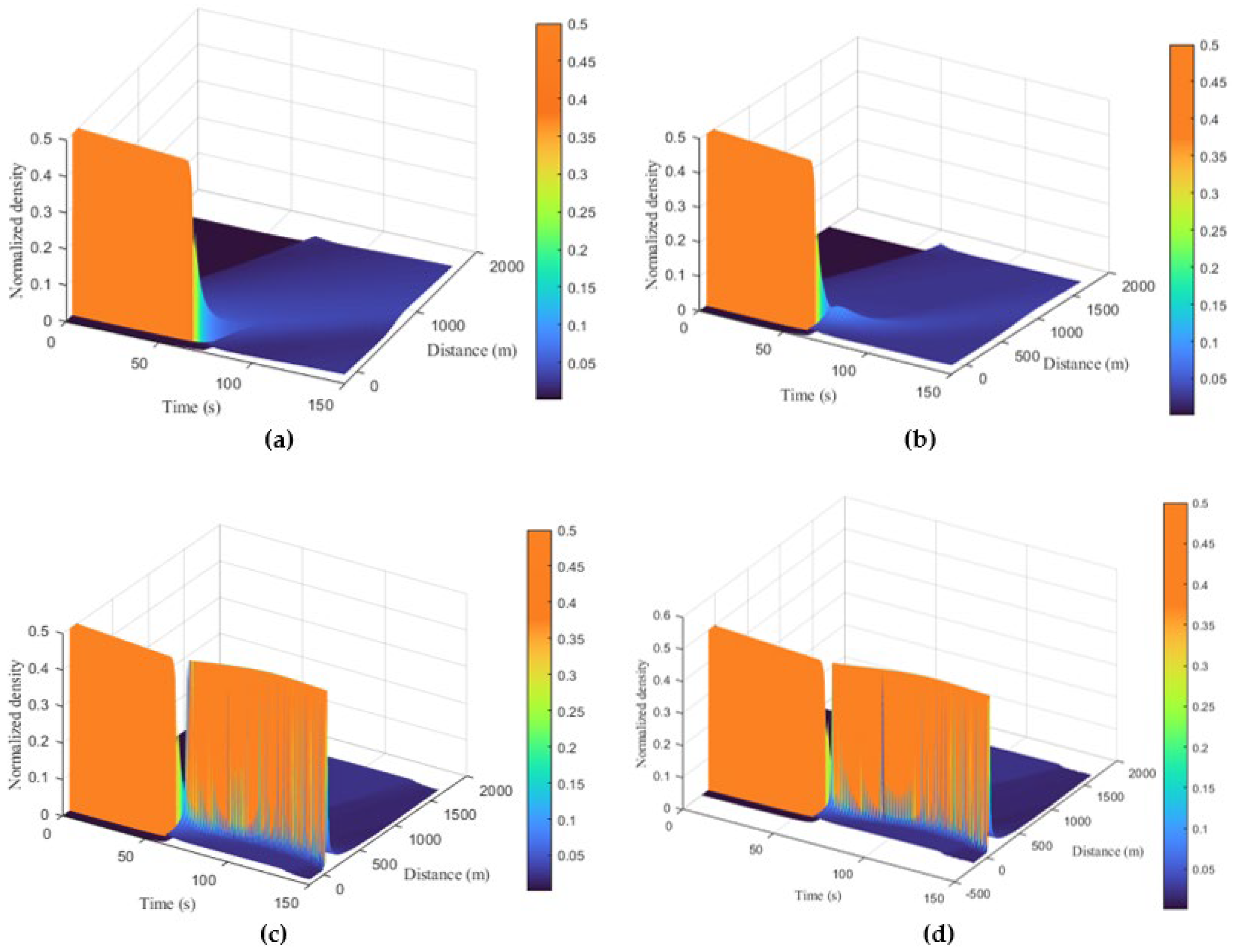
The spatio–temporal density behavior of the ID model is given in Figure 12, and the results are summarized in Table 9. With , between m and m at s, the density is . It increases to at m and at m, then decreases to at m, as shown in Figure 12a. Between s and s at m, the density is , which indicates a traffic queue. After the queue dissolves, the density at s decreases to at m. It then decreases to at m and s. With , between m and m at s, the density is . It increases to at m and then decreases to at m, as shown in Figure 12b. Between s and s at m, the density is , which indicates a traffic queue. After the queue dissolves at s, the density decreases to at m and at m and s. With = 10, between m to m at s, the density is . It increases to between m and m, which indicates a traffic queue. It is at m and decreases to at m, as shown in Figure 12c. Between s and s, the density is , which indicates a traffic queue. It then decreases to at m and s. A queue develops again at s and m with density , which is approximately constant until s between m and m. With = 30, between m and m at s, the density is . It increases to between m and m, which indicates a traffic queue. It is at m and decreases to at m, as shown in Figure 12d. Between s and s, the density is , which indicates a traffic queue. The density then decreases to at m and s. A queue develops again at s and with a density of , which is approximately constant until s between m and m.
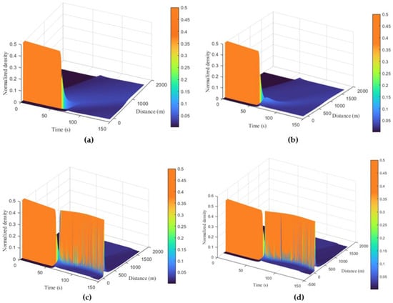
Figure 12.
Spatio–temporal density for the ID model over an m circular road: (a) ; (b) ; (c) ; (d) .

Table 9.
Density and time for the ID model during and after the queue dissolves.
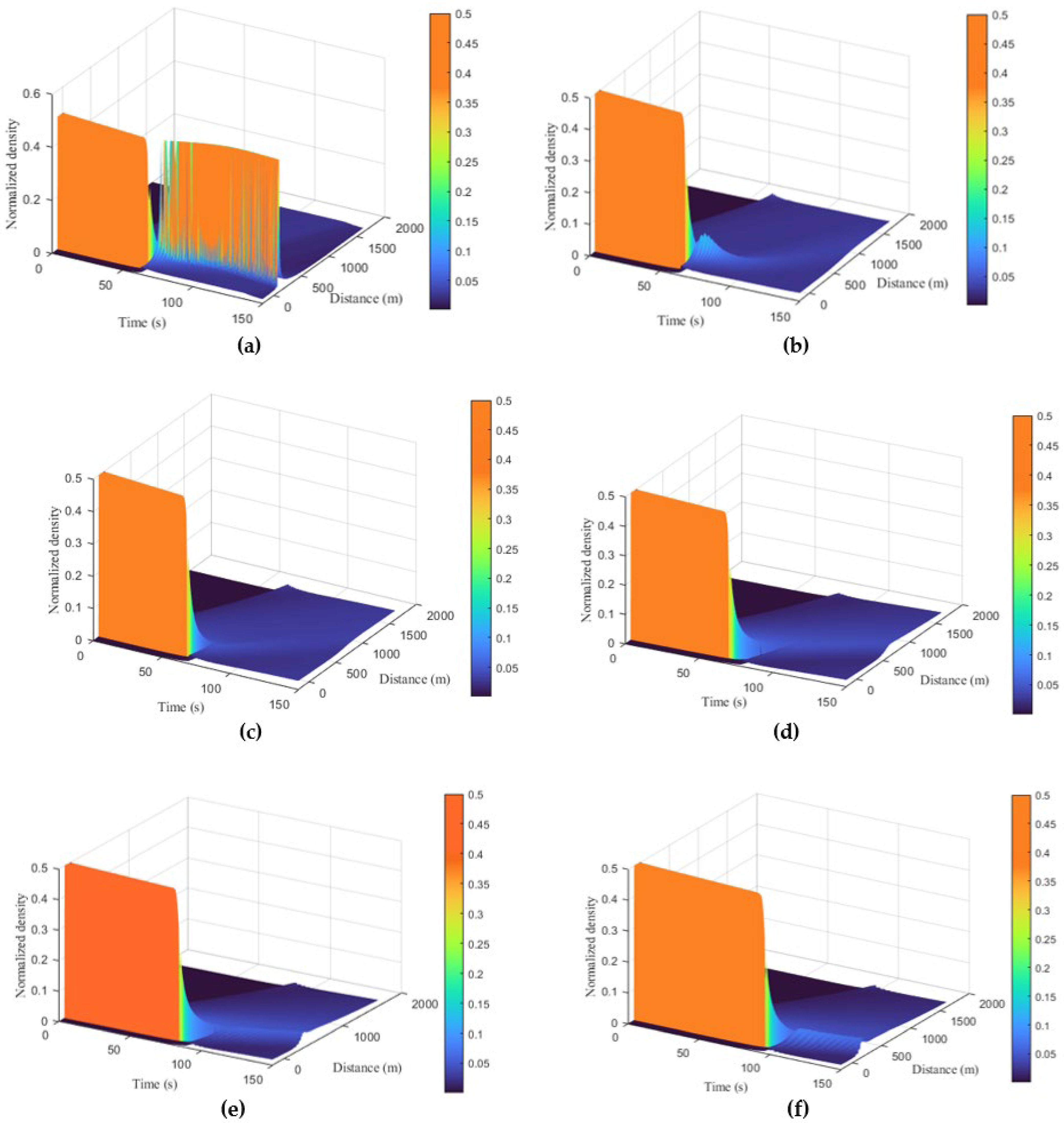
The spatio–temporal density behavior of the proposed model is given in Figure 13, and the results are summarized in Table 10. With m, between m and m at s, the density is . It then increases to between m and m, which indicates a traffic queue. It decreases to at m and at m, as shown in Figure 13a. Between s and s, the density is , which indicates a traffic queue. It then decreases to at m and s. The queue develops again at s and m with a density of and is approximately constant until s between m and m. With m, between m and m at s, the density is . It increases to at m and then decreases to at m, as shown in Figure 13b. Between s and s at m, the density is , which indicates a traffic queue. After the queue dissolves, the density decreases to at − m and s and at m and s. It is at m and s. With m, between m and m at s, the density is . It increases to at m and then decreases to at m, as shown in Figure 13c. Between s and s at m, the density is , which indicates a traffic queue. After the queue dissolves, the density decreases to at − m and s, and at m and s. It then decreases to at m and s. With m, between m and m at s, the density is . It increases to at m and then decreases to at m and to at m, as shown in Figure 13d. Between s and s at m, the density is , which indicates a traffic queue. After the queue dissolves, the density decreases to at − m and s, at m and s, and at m and s. With m, between m and m at s, the density is . It increases to at m, and then it decreases to at m and at m, as shown in Figure 13e. Between s and s at m, the density is , which indicates a traffic queue. After the queue dissolves, the density decreases to at m and s, at m and s, and at m and s. With m, between m and m at s, the density is . It increases to at m, and then decreases to at m, at m, and at , as shown in Figure 13f. Between s and s at , the density is , which indicates a traffic queue. After the queue dissolves, the density decreases to at m and s, at and s, and at m and s.
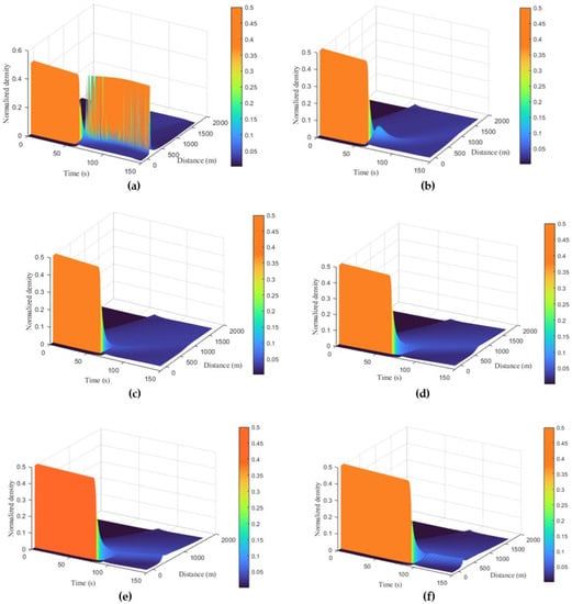
Figure 13.
Spatio–temporal density for the proposed model over an m circular road: (a) m; (b) m; (c) m; (d) m; (e) m; (f) m.

Table 10.
Density and time for the proposed model during and after the queue dissolves.
These results show that the changes in density calculated using the proposed model are small. Density and velocity evolve realistically over time as they are based on the lateral distance headway. The changes in density and velocity calculated using the ID model are based on a constant and increase over time with and , whereas they should decrease. Moreover, for values greater , the behavior is similar, which is not realistic. Further, vehicles move slowly with a larger . With the proposed model, vehicles move based on the lateral distance headway, and they are faster with an increase in this headway. Thus, the flow is smooth with the proposed model and is more realistic than with the ID model. In addition, an increase in the lateral distance headway decreases the variations in acceleration, as expected. With the ID model, an increase in increases the variations in acceleration, which is unrealistic traffic behavior.
5. Conclusions
In this paper, a new heterogeneous traffic model considering the forward and lateral distance headways was proposed. The constant acceleration exponent in the ID model is replaced with an exponent based on realistic traffic parameters to improve the model. It was shown that the ID model produces unrealistic traffic behavior due to a constant exponent. Conversely, the proposed model provides realistic traffic behavior with the velocity and density evolving smoothly over time. Moreover, vehicle movement with the proposed model is faster with a larger lateral distance headway, as expected. With the ID model, this movement is unrealistic because it is based on a constant. Furthermore, it was shown that the proposed model is more stable than the ID model.
With the proposed model, an increase in the lateral distance headway results in small changes in acceleration compared to the ID model. Large acceleration results in high fuel consumption and an increase in pollution. Hence, the proposed model can be utilized to reduce fuel consumption and pollution due to congestion.
Author Contributions
Conceptualization, F.A. and Z.H.K.; methodology, F.A.; software, F.A and A.N.K.; validation, F.A., Z.H.K., K.S.K. and T.A.G.; formal analysis, F.A., Z.H.K., K.S.K. and T.A.G.; investigation, F.A., Z.H.K. and K.S.K.; writing—original draft preparation, F.A.; writing—review and editing, F.A., Z.H.K., K.S.K. and T.A.G.; visualization, F.A., Z.H.K., K.S.K. and T.A.G.; funding acquisition, Z.H.K., K.S.K. and T.A.G. All authors have read and agreed to the published version of the manuscript.
Funding
This research received no external funding.
Conflicts of Interest
The authors declare no conflict of interest.
References
- Timilsina, G.R.; Dulal, H.B. Urban road transportation externalities: Costs and choice of policy instruments. World Bank Res. Obs. 2011, 26, 162–191. [Google Scholar] [CrossRef]
- Chung, K.; Rudjanakanoknad, J.; Cassidy, M.J. Relation between traffic density and capacity drop at three freeway bottlenecks. Transp. Res. Methodol. 2007, 41, 82–95. [Google Scholar] [CrossRef]
- Yuan, K.; Knoop, V.L.; Leclercq, L.; Hoogendoorn, S.P. Capacity drop: A comparison between stop-and-go wave and standing queue at lane-drop bottleneck. Transp. Transp. Dyn. 2017, 5, 145–158. [Google Scholar] [CrossRef]
- Rao, A.M.; Rao, K.R. Measuring urban traffic congestion-a review. Int. J. Traffic Transp. Eng. 2012, 2, 286–305. [Google Scholar]
- Carlson, R.C.; Papamichail, I.; Papageorgiou, M. Local feedback-based mainstream traffic flow control on motorways using variable speed limits. IEEE Trans. Intell. Transp. Syst. 2011, 12, 1261–1276. [Google Scholar] [CrossRef]
- Ali, F.; Khan, Z.H.; Khan, F.A.; Khattak, K.S.; Gulliver, T.A. A new driver model based on driver response. Appl. Sci. 2022, 12, 5390. [Google Scholar] [CrossRef]
- Mallikarjuna, C.; Tharun, B.; Pal, D. Analysis of the lateral gap maintaining behavior of vehicles in heterogeneous traffic stream. Procedia Soc. Behav. Sci. 2013, 104, 370–379. [Google Scholar] [CrossRef]
- Imran, W.; Khan, Z.H.; Gulliver, T.A.; Khattak, K.S.; Nasir, H. A macroscopic traffic model for heterogeneous flow. Chin. J. Phys. 2020, 63, 419–435. [Google Scholar] [CrossRef]
- Khan, Z.H.; Imran, W.; Azeem, S.; Khattak, K.S.; Gulliver, T.A.; Aslam, M.S. A macroscopic traffic model based on driver reaction and traffic stimuli. Appl. Sci. 2019, 9, 2848. [Google Scholar] [CrossRef]
- Adebisi, A. A Review of the Difference among Macroscopic, Microscopic and Mesoscopic Traffic Models; Florida Agricultural and Mechanical University: Tallahassee, FL, USA, 2017. [Google Scholar]
- Khan, Z.H.; Gulliver, T.A.; Khattak, K.S. A novel macroscopic traffic model based on distance headway. Civ. Eng. J. 2021, 7, 32–40. [Google Scholar] [CrossRef]
- Khan, Z.H.; Gulliver, T.A.; Nasir, H.; Rehman, A.; Shahzada, K. A macroscopic traffic model based on driver physiological response. J. Eng. Math. 2019, 115, 21–41. [Google Scholar] [CrossRef]
- Gazis, D.C.; Herman, R.; Rothery, R.W. Nonlinear follow-the-leader models of traffic flow. Oper. Res. 1961, 9, 545–567. [Google Scholar] [CrossRef]
- Newell, G.F. Nonlinear effects in the dynamics of car following. Oper. Res. 1961, 9, 209–229. [Google Scholar] [CrossRef]
- Treiber, M.; Hennecke, A.; Helbing, D. Congested traffic states in empirical observations and microscopic simulations. Phys. Rev. 2000, 62, 1805–1824. [Google Scholar] [CrossRef] [PubMed]
- Newell, G.F. A simplified car-following theory: A lower order model. Transp. Res. Methodol. 2002, 36, 195–205. [Google Scholar] [CrossRef]
- Bando, M.; Hasebe, K.; Nakayama, A.; Shibata, A.; Sugiyama, Y. Dynamical model of traffic congestion and numerical simulation. Phys. Rev. 1995, 51, 1035–1042. [Google Scholar] [CrossRef]
- Helbing, D.; Tilch, B. Generalized force model of traffic dynamics. Phys. Rev. 1998, 58, 133–138. [Google Scholar] [CrossRef]
- Gipps, P.G. A behavioural car-following model for computer simulation. Transp. Res. 1981, 15, 105–111. [Google Scholar] [CrossRef]
- Cao, Z.; Lu, L.; Chen, C.; Chen, X.U. Modeling and simulating urban traffic flow mixed with regular and connected vehicles. IEEE Access 2021, 9, 10392–10399. [Google Scholar] [CrossRef]
- Dahui, W.; Ziqiang, W.; Ying, F. Hysteresis phenomena of the intelligent driver model for traffic flow. Phys. Rev. 2007, 76, 2–8. [Google Scholar] [CrossRef]
- Kesting, A.; Treiber, M.; Helbing, D. Enhanced intelligent driver model to access the impact of driving strategies on traffic capacity. Philos. Trans. R. Soc. Math. Phys. Eng. Sci. 2010, 368, 4585–4605. [Google Scholar] [CrossRef] [PubMed]
- Liebner, M.; Baumann, M.; Klanner, F.; Stiller, C. Driver intent inference at urban intersections using the intelligent driver model. In Proceedings of the IEEE Intelligent Vehicle Symposium, Madrid, Spain, 3–7 June 2012. [Google Scholar]
- Derbel, O.; Peter, T.; Zebiri, H.; Mourllion, B.; Basset, M. Modified intelligent driver model for driver safety and traffic stability improvement. IFAC Proc. 2013, 46, 744–749. [Google Scholar] [CrossRef]
- Li, Y.; Li, Z.; Wang, H.; Wang, W.; Xing, L. Evaluating the safety impact of adaptive cruise control in traffic oscillations on freeways. Accid. Anal. Prev. 2017, 104, 137–145. [Google Scholar] [CrossRef] [PubMed]
- De Winter, J.C.F.; Happee, R.; Martens, M.H.; Stanton, N.A. Effects of adaptive cruise control and highly automated driving on workload and situation awareness: A review of the empirical evidence. Transp. Res. Psychol. Behav. 2014, 27, 196–217. [Google Scholar] [CrossRef]
- Jafaripournimchahi, A.; Cai, Y.; Wang, H.; Sun, L.; Weng, J. Integrated-hybrid framework for connected and autonomous vehicles microscopic traffic flow modelling. J. Adv. Transp. 2002, 2022, 2253697. [Google Scholar] [CrossRef]
- Lu, X.; Wang, Z.; Xu, M.; Chen, W.; Deng, Z. A personality model for animating heterogeneous traffic behaviors. Comput. Animat. Virtual Worlds 2014, 25, 361–371. [Google Scholar] [CrossRef]
- Gao, Z.; Wang, J.; Zhang, X.; Dong, J.; Chen, L.; Yan, X.; Zhang, W. Traffic oscillations mitigation in vehicle platoon using a car-following control model for connected and autonomous vehicle. J. Adv. Transp. 2019, 2019, 3067291. [Google Scholar] [CrossRef]
- Dey, P.P.; Chandra, S.; Gangopadhyay, S. Simulation of mixed traffic flow on two-lane roads. J. Transp. Eng. 2008, 134, 361–369. [Google Scholar] [CrossRef]
- Gunay, B. Car following theory with lateral discomfort. Transp. Res. Methodol. 2007, 41, 722–735. [Google Scholar] [CrossRef]
- Metkari, M.; Budhkar, A.; Maurya, A.K. Development of simulation model for heterogeneous traffic with no lane discipline. Procedia Soc. Behav. Sci. 2013, 104, 360–369. [Google Scholar] [CrossRef][Green Version]
- Mohan, R.; Ramadurai, G. Heterogeneous traffic flow modelling using second-order macroscopic continuum model. Phys. Lett. 2017, 381, 115–123. [Google Scholar] [CrossRef]
- Stern, R.E.; Cui, S.; Delle Monache, M.L.; Bhadani, R.; Bunting, M.; Churchill, M.; Hamilton, N.; Pohlmann, H.; Wu, F.; Piccoli, B.; et al. Dissipation of stop-and-go waves via control of autonomous vehicles: Field experiments. Transp. Res. Emerg. Technol. 2018, 89, 205–221. [Google Scholar] [CrossRef]
- Hu, X.; Chiu, Y.C.; Ma, Y.L.; Zhu, L. Studying driving risk factors using multi-source mobile computing data. Int. J. Transp. Sci. Technol. 2015, 4, 295–312. [Google Scholar] [CrossRef]
- Malinauskas, R. The Intelligent Driver Model: Analysis and Application to Adaptive Cruise Control. Ph.D. Thesis, Clemson University, Clemson, SC, USA, 2014. [Google Scholar]
- Kessels, F. Traffic Flow Modelling: Introduction to Traffic Flow Theory through a Genealogy of Models; Springer: Cham, Switzerland, 2019. [Google Scholar]
- Khansari, E.R.; Tabibi, M.; Nejad, F.M. A study on following behavior based on the time headway. J. Kejuruter. 2020, 32, 187–195. [Google Scholar]
- Toledo, T.; Koutsopoulos, H.N.; Ben-Akiva, M. Integrated driving behavior modeling. Transp. Res. Emerg. Technol. 2007, 15, 96–112. [Google Scholar] [CrossRef]
- Imran, W.; Khan, Z.H.; Gulliver, T.A.; Khattak, K.S.; Saeed, S.; Aslam, M.S. Macroscopic traffic flow characterization for stimuli based on driver reaction. Civ. Eng. J. 2021, 7, 1–13. [Google Scholar] [CrossRef]
Disclaimer/Publisher’s Note: The statements, opinions and data contained in all publications are solely those of the individual author(s) and contributor(s) and not of MDPI and/or the editor(s). MDPI and/or the editor(s) disclaim responsibility for any injury to people or property resulting from any ideas, methods, instructions or products referred to in the content. |
© 2022 by the authors. Licensee MDPI, Basel, Switzerland. This article is an open access article distributed under the terms and conditions of the Creative Commons Attribution (CC BY) license (https://creativecommons.org/licenses/by/4.0/).


