Solutions to the (4+1)-Dimensional Time-Fractional Fokas Equation with M-Truncated Derivative

Abstract

In this paper, we consider the (4+1)-dimensional fractional Fokas equation (FFE) with an M-truncated derivative. The extended tanh–coth method and the Jacobi elliptic function method are utilized to attain new hyperbolic, trigonometric, elliptic, and rational fractional solutions. In addition, we generalize some previous results. The acquired solutions are beneficial in analyzing definite intriguing physical phenomena because the FFE equation is crucial for explaining various phenomena in optics, fluid mechanics and ocean engineering. To demonstrate how the M-truncated derivative affects the analytical solutions of the FFE, we simulate our figures in MATLAB and show several 2D and 3D graphs.

1. Introduction

In electromagnetic theory, engineering disciplines, mathematical biology, signal processing, and other scientific research, fractional differential equations (FDEs) are used to interpret a wide range of physical phenomena [1,2,3,4,5]. Moreover, the fractional-order derivative describe many physical phenomena including quantum mechanics, gravity, diffusion, electrodynamics, fluid dynamics, sound electrostatics, elasticity, heat, and so on. Due to the significant of the fractional-order derivative, many definitions have been investigated, such as the Grunwald–Letnikov derivative, the Caputo derivative, the new truncated M-fractional derivative, conformable fractional definitions, an Atangana–Baleanu derivative in the context of Caputo, He’s fractional derivative, the Riesz derivative, the Weyl derivative, and the Riemann–Liouville derivative [6,7,8,9,10,11,12,13].

The importance of FDEs has led to the development of numerous effective and potent techniques for discovering exact solutions to those equations. Some of these techinques include the Riccati–Bernoulli sub-ODE [14], the tanh–sech [15,16], the Jacobi elliptic function [17], Hirota’s method [18], the $exp(-\varphi (\varsigma \left)\right)$-expansion method [19], the perturbation method [20,21], the sine–cosine method [22,23], the $(G^{\prime }/G)$-expansion method [24,25], etc.

There are some study about the fractional Laplacian derivative, such as [26,27,28]. However, here, we are interested in the following (4+1)-dimensional fractional Fokas equation (FFE) with a time derivative:

$$4_0{D}_{M,t}^{\alpha ,\beta }{\psi }_x-{\psi }_{xxxy}+{\psi }_{xyyy}+12{\psi }_x{\psi }_y+12\psi {\psi }_{xy}-6{\psi }_{zw}=0,$$

(1)

where $\psi =\psi (x,y,z,\omega ,t)$ is a higher-dimensional nonlinear wave equation that Fokas [29] derived by extending the Davey–Stewartson equation (DSE) and the Kadomtsev–Petviashvili equation (KPE). The DSE and KPE are suggested in nonlinear wave theory to describe surface waves and internal waves in straits or channels of varied depth and breadth [30],as well as the development of a three-dimensional wave-packet on water of limited depth [31]. ${}_0{D}_{M,t}^{\alpha ,\beta }$ is the M-truncated derivative and is defined in the next section.

In mathematical physics, the (4+1)-dimensional Fokas equation is regarded as an integrable higher-dimensional problem. The significance of the Fokas Equation (1) indicates that the presence of nonlinear integrable equations in special four dimensions including complex time may be examined in the framework of recent field theories [29]. Equation (1) can be employed to describe different phenomena in ocean engineering, fluid mechanics, and optics. Additionally, it can explain elastic and inelastic interactions. With $\alpha =1$ and $\beta =0,$ several methods can be used to obtain exact solutions of the Fokas Equation (1) such as truncated Painlevè expansion [32], extended F-expansion [33], the Hirota bilinear method [34], a modified simple equation [35], $(G^{\prime }/G)$-expansion [36], tanh–coth [37], the improved F-expansion method [38],etc. Moreover, Yang and Yan [39] discussed the Lie point symmetries and potential symmetries of this model, while Lu et al. [40] studied the symmetry property of the time fractional Equation (1), and Ullah et al. [41] used the Sardar subequation method for a space–time fractional-order Equation (1) with a conformable derivative.

Our motivation for this paper is to find the exact solutions of FFE (1) with an M-truncated derivative. We utilize the extended tanh–coth method and the Jacobi elliptic function method to acquire these solutions. Additionally, we extend some earlier studies such as the results reported in [33,35,36]. The solutions offered are incredibly helpful to physicists in describing several significant physical problems. Moreover, we display the impact of a fractional derivative on the analytical solution of the FFE (1) by presenting several graphical representations using the MATLAB tools.

The article is structured as follows: In Section 2, the M-truncated derivative is defined, and its features are given. In Section 3, we utilize the wave transformation to attain the wave equation for the FFE (1). In Section 4, we obtain the exact fractional solutions of the FFE (1), while in Section 5, we introduce some graphs to see the impact of fractional derivative on the acquired solutions of the FFE. Finally, the article’s conclusions are introduced.

2. M-Truncated Derivative

In [13], Sousa et al. have investigated a new fractional derivative called the M-truncated derivative (M-TD). The M-TD satisfies some features of classical calculus, e.g., chain rule, function composition rule, quotient rule, product rule, and linearity. From this point, let us define the truncated Mittag–Leffler function with one parameter, as follows:

Definition 1 

([13,42]). The truncated Mittag–Leffler function is defined, for $\beta >0$ and $y\in \mathbb{C}$, as

$${}_i{E}_{\beta }\left(y\right)=\sum _{k=0}^i\frac{y^k}{\mathrm{\Gamma }(\beta k+1)}.$$

Definition 2 

([13,42]). The M-TD for the function $\phi :[0,\infty )\to \mathbb{R}$ of order $\alpha \in (0,1)$ is defined as

$${}_i{D}_{M,t}^{\alpha ,\beta }\phi \left(t\right)=\underset{h\to 0}{lim}\frac{\phi \left(t{+}_i{E}_{\beta }\left(h{t}^{-\alpha }\right)\right)-\phi \left(t\right)}{h},$$

for $t>0$.

Theorem 1 

([13,42]). If φ and ψ are differentiable functions, then, for a, $b,\upsilon$ are real constants, we have

(1)

${}_i{D}_{M,x}^{\alpha ,\beta }(a\phi +b\psi )=a_i{D}_{M,x}^{\alpha ,\beta }\left(\phi \right)+b_i{D}_{M,x}^{\alpha ,\beta }\left(\psi \right);$

(2)

${}_i{D}_{M,x}^{\alpha ,\beta }\left(x^{\nu }\right)=\frac{\nu }{\mathrm{\Gamma }(\beta +1)}{x}^{\nu -\alpha }$;

(3)

${}_i{D}_{M,x}^{\alpha ,\beta }\left(\phi \psi \right)={\phi }_i{D}_{M,x}^{\alpha ,\beta }\psi +{\psi }_i{D}_{M,x}^{\alpha ,\beta }\phi ;$

(4)

${}_i{D}_{M,x}^{\alpha ,\beta }\left(\phi \right)\left(x\right)=\frac{x^{1-\alpha }}{\mathrm{\Gamma }(\beta +1)}\frac{d\phi }{dx}$;

(5)

${}_i{D}_{M,x}^{\alpha ,\beta }(\phi \circ \psi )\left(x\right)={\phi }^{{}^{\prime }}{\left(\psi \left(x\right)\right)}_i{D}_{M,x}^{\alpha ,\beta }\psi \left(x\right)$.

3. Wave Equation for the FFE

The next wave transformation is used to generate the wave equation for FFE FFE (1):

$$\psi (x,y,z,\omega ,t)=\phi \left(\xi \right),\xi ={\xi }_{1}x+{\xi }_{2}y+{\xi }_{3}z+{\xi }_4\omega +\frac{\lambda \mathrm{\Gamma }(\beta +1)}{\alpha }{t}^{\alpha },$$

(2)

where $\phi$ is a real function, ${\xi }_1,{\xi }_2,{\xi }_3,{\xi }_4$ and $\lambda$ are non-zero constants. We note that

$${\psi }_x={\xi }_1{\phi }^{\prime },{\psi }_y={\xi }_2{\phi }^{\prime },$$

(3)

$${}_0{D}_{M,t}^{\alpha ,\beta }{\psi }_x=\lambda {\xi }_1{\phi }^{″},{\psi }_{xy}={\xi }_1{\xi }_2{\phi }^{″},{\psi }_{z\omega }={\xi }_3{\xi }_4{\phi }^{″},$$

(4)

and

$${\psi }_{xxxy}={\xi }_1^3{\xi }_2{\phi }^{\left(4\right)},{\psi }_{xyyy}={\xi }_1{\xi }_2^3{\phi }^{\left(4\right)}.$$

(5)

Plugging Equation (2) into Equation (1) and using (3)–(5), we have

$$[4\lambda {\xi }_1-6{\xi }_3{\xi }_4]{\phi }^{″}+[{\xi }_1{\xi }_2^3-{\xi }_1^3{\xi }_2]{\phi }^{\left(4\right)}+12{\xi }_1{\xi }_2{\left(\phi {\phi }^{\prime }\right)}^{\prime }=0,$$

(6)

where ${\left({\phi }^{\prime }\right)}^2+\phi {\phi }^{″}={\left(\phi {\phi }^{\prime }\right)}^{\prime }.$ Integrating Equation (6) twice and putting the integration constants equal to zero, we have

$${\phi }^{″}+{\gamma }_1\phi +{\gamma }_2{\phi }^2=0,$$

(7)

where

$${\gamma }_1=\frac{4\lambda {\xi }_1-6{\xi }_3{\xi }_4}{{\xi }_1{\xi }_2^3-{\xi }_1^3{\xi }_2}\mathrm{and}{\gamma }_2=\frac{6}{{\xi }_2^2-{\xi }_1^2}.$$

4. Exact Solutions of FFE

In this section, we apply two methods, the extended tanh–coth and the Jacobi elliptic function methods, in order to obtain the fractional solutions for FFE (1).

4.1. Extended Tanh–Coth Method

Here, we use the extended tanh–coth method (for more information, see [16]). Let us assume the solution $\phi$ of Equation (7) has the form

$$\phi \left(\xi \right)=\sum _{j=0}^M{a}_j{\varphi }^j+\sum _{j=1}^M{b}_j{\varphi }^{-j},$$

(8)

where $\varphi$ solves

$${\varphi }^{\prime }={\varphi }^2+k.$$

(9)

The solutions of Equation (9) are: If $k>0,$ we have

$$\varphi \left(\xi \right)=\sqrt{k}tan\left(\sqrt{k}\xi \right)\mathrm{or}\varphi \left(\xi \right)=-\sqrt{k}cot\left(\sqrt{k}\xi \right).$$

(10)

If $k<0,$ we have

$$\varphi \left(\xi \right)=-\sqrt{-k}tanh\left(\sqrt{-k}\xi \right)\mathrm{or}\varphi \left(\xi \right)=-\sqrt{-k}coth\left(\sqrt{-k}\xi \right).$$

(11)

If $k=0,$ we have

$$\varphi \left(\xi \right)=\frac{-1}{\xi }.$$

(12)

To calculate the parameter M, we balance ${\phi }^2$ with ${\phi }^{″}$ in Equation (7) to obtain

$$2M=M+2,$$

hence

$$M=2.$$

(13)

Rewrite Equation (8) using Equation (13) as

$$\phi \left(\xi \right)=a_0+a_1\varphi +a_2{\varphi }^2+b_1{\varphi }^{-1}+b_2{\varphi }^{-2}.$$

(14)

Substituting Equation (14) into Equation (7), we obtain

$$\begin{array}{c}(6k{a}_2+{\gamma }_2{a}_2^2){\varphi }^4+(2a_1+2{\gamma }_2{a}_1{a}_2){\varphi }^3+(8k{a}_2+2a_0{a}_2{\gamma }_2+a_1^2{\gamma }_2+{\gamma }_1{a}_2){\varphi }^2\hfill \\ (2k{a}_1+{\gamma }_1{a}_1+2{\gamma }_2{a}_0{a}_1+2a_2{b}_1)\varphi +(2k^2{a}_2+2b_2+{\gamma }_1{a}_0+{\gamma }_2{a}_0^2+2{\gamma }_2{a}_1{b}_1\hfill \\ +2{\gamma }_2{a}_2{b}_2)+(2k{b}_1+2{\gamma }_2{a}_0{b}_1+2{\gamma }_2{a}_1{b}_2+{\gamma }_1{b}_1){\varphi }^{-1}+(8k{b}_2+2a_0{b}_2{\gamma }_2\hfill \\ +b_1^2{\gamma }_2+{\gamma }_1{b}_2){\varphi }^{-2}+(2b_1{k}^2+2{\gamma }_2{b}_1{b}_2){\varphi }^{-3}+(6k^2{b}_2+{\gamma }_2{b}_2^2){\varphi }^4=0.\end{array}$$

Set the coefficients of each power of $\varphi$ to zero as follows:

$$6a_2+{\gamma }_2{a}_2^2=0,$$

$$2a_1+2{\gamma }_2{a}_1{a}_2=0,$$

$$8k{a}_2+2a_0{a}_2{\gamma }_2+a_1^2{\gamma }_2+{\gamma }_1{a}_2=0,$$

$$2k{a}_1+{\gamma }_1{a}_1+2{\gamma }_2{a}_0{a}_1+2a_2{b}_1=0,$$

$$2k^2{a}_2+2b_2+{\gamma }_1{a}_0+{\gamma }_2{a}_0^2+2{\gamma }_2{a}_1{b}_1+2{\gamma }_2{a}_2{b}_2=0,$$

$$2k{b}_1+2{\gamma }_2{a}_0{b}_1+2{\gamma }_2{a}_1{b}_2+{\gamma }_1{b}_1=0,$$

$$8k{b}_2+2a_0{b}_2{\gamma }_2+b_1^2{\gamma }_2+{\gamma }_1{b}_2=0,$$

$$2b_1{k}^2+2{\gamma }_2{b}_1{b}_2=0.$$

and

$$6k^2{b}_2+{\gamma }_2{b}_2^2=0.$$

Solving these equations, we attain the following four different sets:

First set:

$$a_0=\frac{-6k}{{\gamma }_2},a_1=0,a_2=\frac{-6}{{\gamma }_2},b_1=0,b_2=0,\lambda =\frac{3{\xi }_3{\xi }_4+2k[{\xi }_1{\xi }_2^3-{\xi }_1^3{\xi }_2]}{2{\xi }_1}.$$

(15)

Second set:

$$a_0=\frac{-2k}{{\gamma }_2},a_1=0,a_2=\frac{-6}{{\gamma }_2},b_1=0,b_2=0,\lambda =\frac{3{\xi }_3{\xi }_4-2k[{\xi }_1{\xi }_2^3-{\xi }_1^3{\xi }_2]}{2{\xi }_1}.$$

(16)

Third set:

$$a_0=\frac{-12k}{{\gamma }_2},a_1=0,a_2=\frac{-6}{{\gamma }_2},b_1=0,b_2=\frac{-6k^2}{{\gamma }_2},\lambda =\frac{3{\xi }_3{\xi }_4+8k[{\xi }_1{\xi }_2^3-{\xi }_1^3{\xi }_2]}{2{\xi }_1}.$$

(17)

Fourth set:

$$a_0=\frac{8k}{{\gamma }_2},a_1=0,a_2=\frac{-6}{{\gamma }_2},b_1=0,b_2=\frac{-6k^2}{{\gamma }_2},\lambda =\frac{3{\xi }_3{\xi }_4-8k[{\xi }_1{\xi }_2^3-{\xi }_1^3{\xi }_2]}{2{\xi }_1}.$$

(18)

First set: In this set, the Equation (7) has the solution

$$\phi \left(\xi \right)=\frac{-6k}{{\gamma }_2}-\frac{6}{{\gamma }_2}{\varphi }^2\left(\xi \right).$$

For $\varphi \left(\xi \right)$, there are three cases:

Case 1: If $k>0,$ then by using (10), we have

$$\phi \left(\xi \right)=\frac{-6k}{{\gamma }_2}-\frac{6k}{{\gamma }_2}{tan}^2\left(\sqrt{k}\xi \right)=-\frac{6k}{{\gamma }_2}{sec}^2\left(\sqrt{k}\xi \right),$$

and

$$\phi \left(\xi \right)=\frac{-6k}{{\gamma }_2}-\frac{6k}{{\gamma }_2}{cot}^2\left(\sqrt{k}\xi \right)=\frac{-6k}{{\gamma }_2}{csc}^2\left(\sqrt{k}\xi \right).$$

Thus, the fractional exact solution of FFE (1) is

$$\psi (x,y,z,\omega ,t)=-\frac{6k}{{\gamma }_2}{sec}^2\left(\sqrt{k}\xi \right),$$

(19)

and

$$\psi (x,y,z,\omega ,t)=\frac{-6k}{{\gamma }_2}{csc}^2\left(\sqrt{k}\xi \right),$$

(20)

where $\xi ={\xi }_{1}x+{\xi }_{2}y+{\xi }_{3}z+{\xi }_4\omega +\frac{\mathrm{\Gamma }(\beta +1)[3{\xi }_3{\xi }_4+2k({\xi }_1{\xi }_2^3-{\xi }_1^3{\xi }_2)]}{2{\xi }_1\alpha }{t}^{\alpha }.$

Case 2: If $k<0,$ then by using (11), we have

$$\phi \left(\xi \right)=\frac{-6k}{{\gamma }_2}+\frac{6k}{{\gamma }_2}{tanh}^2\left(\sqrt{-k}\xi \right)=\frac{-6k}{{\gamma }_2}{\mathrm{sech}}^2\left(\sqrt{-k}\xi \right),$$

and

$$\phi \left(\xi \right)=\frac{-6k}{{\gamma }_2}+\frac{6k}{{\gamma }_2}{coth}^2\left(\sqrt{-k}\xi \right)=\frac{6k}{{\gamma }_2}{\mathrm{csch}}^2\left(\sqrt{-k}\xi \right).$$

Thus, the fractional exact solution of FFE (1) is

$$\psi (x,y,z,\omega ,t)=\frac{-6k}{{\gamma }_2}{\mathrm{sech}}^2\left(\sqrt{-k}\xi \right),$$

(21)

and

$$\psi (x,y,z,\omega ,t)=\frac{6k}{{\gamma }_2}{\mathrm{csch}}^2\left(\sqrt{-k}\xi \right).$$

(22)

Case 3: If $k=0,$ then by using (12), we have

$$\phi \left(\xi \right)=\frac{6}{{\gamma }_2}\frac{1}{{\xi }^2}.$$

Thus, the fractional exact solution of FFE (1) is

$$\psi (x,y,z,\omega ,t)=[-\frac{6}{{\gamma }_2}\frac{1}{{\xi }^2}],$$

(23)

where $\xi ={\xi }_{1}x+{\xi }_{2}y+{\xi }_{3}z+{\xi }_4\omega +\frac{\mathrm{\Gamma }(\beta +1)[3{\xi }_3{\xi }_4+2k({\xi }_1{\xi }_2^3-{\xi }_1^3{\xi }_2)]}{2{\xi }_1\alpha }{t}^{\alpha }.$

Second set: The solution of Equation (7) in this set is

$$\phi \left(\xi \right)=\frac{-2k}{{\gamma }_2}-\frac{6}{{\gamma }_2}{\varphi }^2\left(\xi \right).$$

For $\varphi \left(\xi \right)$, there are three cases:

Case 1: If $k>0,$ then by using (10), we have

$$\phi \left(\xi \right)=\frac{-2k}{{\gamma }_2}-\frac{6k}{{\gamma }_2}{tan}^2\left(\sqrt{k}\xi \right),$$

and

$$\phi \left(\xi \right)=\frac{-2k}{{\gamma }_2}-\frac{6k}{{\gamma }_2}{cot}^2\left(\sqrt{k}\xi \right).$$

Thus, the fractional exact solution of FFE (1) is

$$\psi (x,y,z,\omega ,t)=[\frac{-2k}{{\gamma }_2}-\frac{6k}{{\gamma }_2}{tan}^2\left(\sqrt{k}\xi \right)],$$

(24)

and

$$\psi (x,y,z,\omega ,t)=[\frac{-2k}{{\gamma }_2}-\frac{6k}{{\gamma }_2}{cot}^2\left(\sqrt{k}\xi \right)],$$

(25)

where $\xi ={\xi }_{1}x+{\xi }_{2}y+{\xi }_{3}z+{\xi }_4\omega +\frac{\mathrm{\Gamma }(\beta +1)[3{\xi }_3{\xi }_4-2k({\xi }_1{\xi }_2^3-{\xi }_1^3{\xi }_2)]}{2{\xi }_1\alpha }{t}^{\alpha }.$

Case 2: If $k<0,$ then by using (11), we have

$$\phi \left(\xi \right)=\frac{-2k}{{\gamma }_2}+\frac{6k}{{\gamma }_2}{tanh}^2\left(\sqrt{-k}\xi \right),$$

and

$$\phi \left(\xi \right)=\frac{-2k}{{\gamma }_2}+\frac{6k}{{\gamma }_2}{coth}^2\left(\sqrt{-k}\xi \right).$$

Thus, the fractional exact solution of FFE (1) is

$$\psi (x,y,z,\omega ,t)=\frac{-2k}{{\gamma }_2}+\frac{6k}{{\gamma }_2}{tanh}^2\left(\sqrt{-k}\xi \right),$$

(26)

and

$$\psi (x,y,z,\omega ,t)=\frac{-2k}{{\gamma }_2}+\frac{6k}{{\gamma }_2}{coth}^2\left(\sqrt{-k}\xi \right).$$

(27)

Case 3: If $k=0,$ then by using (12), we have

$$\phi \left(\xi \right)=\frac{6}{{\gamma }_2}\frac{1}{{\xi }^2}.$$

Thus, the fractional exact solution of FFE (1) is

$$\psi (x,y,z,\omega ,t)=\frac{6}{{\gamma }_2}\frac{1}{{\xi }^2},$$

(28)

where $\xi ={\xi }_{1}x+{\xi }_{2}y+{\xi }_{3}z+{\xi }_4\omega +\frac{\mathrm{\Gamma }(\beta +1)[3{\xi }_3{\xi }_4-2k({\xi }_1{\xi }_2^3-{\xi }_1^3{\xi }_2)]}{2{\xi }_1\alpha }{t}^{\alpha }.$

Third set: In this set, the Equation (7) has the solution

$$\phi \left(\xi \right)=\frac{-12k}{{\gamma }_2}-\frac{6}{{\gamma }_2}{\varphi }^2\left(\xi \right)-\frac{6k^2}{{\gamma }_2}{\varphi }^{-2}\left(\xi \right).$$

For $\varphi \left(\xi \right)$, there are three cases:

Case 1: If $k>0,$ then by using (10), we have

$$\begin{array}{ccc}\hfill \phi \left(\xi \right)& =& \frac{-12k}{{\gamma }_2}-\frac{6k}{{\gamma }_2}{tan}^2\left(\sqrt{k}\xi \right)-\frac{6k}{{\gamma }_2}{cot}^2\left(\sqrt{k}\xi \right)\hfill \\ & =& -\frac{6k}{{\gamma }_2}[{sec}^2\left(\sqrt{k}\xi \right)+{csc}^2\left(\sqrt{k}\xi \right)].\hfill \end{array}$$

Thus, the fractional exact solution of FFE (1) is

$$\psi (x,y,z,\omega ,t)=-\frac{6k}{{\gamma }_2}[{sec}^2\left(\sqrt{k}\xi \right)+{csc}^2\left(\sqrt{k}\xi \right)],$$

(29)

where $\xi ={\xi }_{1}x+{\xi }_{2}y+{\xi }_{3}z+{\xi }_4\omega +\frac{\mathrm{\Gamma }(\beta +1)[3{\xi }_3{\xi }_4+8k({\xi }_1{\xi }_2^3-{\xi }_1^3{\xi }_2)]}{2{\xi }_1\alpha }{t}^{\alpha }.$

Case 2: If $k<0,$ then by using (11), we have

$$\begin{array}{ccc}\hfill \phi \left(\xi \right)& =& \frac{-12k}{{\gamma }_2}+\frac{6k}{{\gamma }_2}{tanh}^2(\sqrt{-k}\xi )+\frac{6k}{{\gamma }_2}{coth}^2(\sqrt{-k}\xi )\hfill \\ & =& \frac{-6k}{{\gamma }_2}[{\mathrm{sech}}^2(\sqrt{-k}\xi )-{\mathrm{csch}}^2(\sqrt{-k}\xi )].\hfill \end{array}$$

Thus, the fractional exact solution of FFE (1) is

$$\psi (x,y,z,\omega ,t)=\frac{-6k}{{\gamma }_2}[{\mathrm{sech}}^2(\sqrt{-k}\xi )-{\mathrm{csch}}^2(\sqrt{-k}\xi )],$$

(30)

where $\xi ={\xi }_{1}x+{\xi }_{2}y+{\xi }_{3}z+{\xi }_4\omega +\frac{\mathrm{\Gamma }(\beta +1)[3{\xi }_3{\xi }_4+8k({\xi }_1{\xi }_2^3-{\xi }_1^3{\xi }_2)]}{2{\xi }_1\alpha }{t}^{\alpha }.$

Case 3: If $k=0,$ then by using (12), we have

$$\phi \left(\xi \right)=\frac{6}{{\gamma }_2}\frac{1}{{\xi }^2}+\frac{6}{{\gamma }_2}{\xi }^2.$$

Thus, the fractional exact solution of FFE (1) is

$$\psi (x,y,z,\omega ,t)=\frac{6}{{\gamma }_2}\frac{1}{{\xi }^2}+\frac{6}{{\gamma }_2}{\xi }^2.$$

(31)

Fourth set: In this set, the Equation (7) has the solution

$$\phi \left(\xi \right)=\frac{8k}{{\gamma }_2}-\frac{6}{{\gamma }_2}{\varphi }^2\left(\xi \right)-\frac{6k^2}{{\gamma }_2}{\varphi }^{-2}\left(\xi \right).$$

For $\varphi \left(\xi \right)$, there are three cases:

Case 1: If $k>0,$ then by using (10), we have

$$\phi \left(\xi \right)=\frac{8k}{{\gamma }_2}-\frac{6k}{{\gamma }_2}{tan}^2\left(\sqrt{k}\xi \right)-\frac{6k}{{\gamma }_2}{cot}^2\left(\sqrt{k}\xi \right).$$

Thus, the fractional exact solution of FFE (1) is

$$\psi (x,y,z,\omega ,t)=\frac{8k}{{\gamma }_2}-\frac{6k}{{\gamma }_2}{tan}^2\left(\sqrt{k}\xi \right)-\frac{6k}{{\gamma }_2}{cot}^2\left(\sqrt{k}\xi \right),$$

(32)

where $\xi ={\xi }_{1}x+{\xi }_{2}y+{\xi }_{3}z+{\xi }_4\omega +\frac{\mathrm{\Gamma }(\beta +1)[3{\xi }_3{\xi }_4-8k({\xi }_1{\xi }_2^3-{\xi }_1^3{\xi }_2)]}{2{\xi }_1\alpha }{t}^{\alpha }.$

Case 2: If $k<0,$ then by using (11), we have

$$\phi \left(\xi \right)=\frac{8k}{{\gamma }_2}+\frac{6k}{{\gamma }_2}{tanh}^2\left(\sqrt{-k}\xi \right)+\frac{6k}{{\gamma }_2}{coth}^2\left(\sqrt{-k}\xi \right).$$

Thus, the fractional exact solution of FFE (1) is

$$\psi (x,y,z,\omega ,t)=\frac{8k}{{\gamma }_2}+\frac{6k}{{\gamma }_2}{tanh}^2(\sqrt{-k}\xi )+\frac{6k}{{\gamma }_2}{coth}^2(\sqrt{-k}\xi ).$$

(33)

Case 3: If $k=0,$ then by using (12), we have

$$\phi \left(\xi \right)=\frac{6}{{\gamma }_2}\frac{1}{{\xi }^2}+\frac{6}{{\gamma }_2}{\xi }^2.$$

Thus, the fractional exact solution of FFE (1) is

$$\psi (x,y,z,\omega ,t)=\frac{6}{{\gamma }_2}\frac{1}{{\xi }^2}+\frac{6}{{\gamma }_2}{\xi }^2,$$

(34)

where $\xi ={\xi }_{1}x+{\xi }_{2}y+{\xi }_{3}z+{\xi }_4\omega +\frac{\mathrm{\Gamma }(\beta +1)\left[3{\xi }_3{\xi }_4\right]}{2{\xi }_1\alpha }{t}^{\alpha }.$

Remark 1. 

Putting $\alpha =1$ in Equations (21), (22), (26), and (27), we attain the same solutions (36), (37), (45), and (46), respectively, declared in [35] by the modified simple equation method.

Remark 2. 

Putting $\alpha =1$ in Equations (21), we obtain the same solution (10) declared in [36] by the $(G^{\prime }/G)$-expansion method.

Remark 3. 

Putting $\alpha =1$ in Equations (19), (30), and (33), we obtain the same solutions (17), (29), and (23) stated in [33] by the extended F-expansion method.

4.2. Jacobi Elliptic Function Method

In this subsection, we use the Jacobi elliptic function method (for more information, see [43]). Considering the solutions to Equation (7) takes the next type (with $M=2$):

$$\phi \left(\xi \right)={\hslash }_0+{\hslash }_1\mathrm{\Omega }\left(\xi \right)+{\hslash }_2{\mathrm{\Omega }}^2\left(\xi \right),$$

(35)

where $\mathrm{\Omega }\left(\xi \right)=sn(\xi ,m)$ is a Jacobi elliptic sine function for $0<m<1$ and ${\hslash }_0,{\hslash }_1$, and ${\hslash }_2$ are unknown constants. Differentiating Equation (35) twice

$${\phi }^{″}\left(\xi \right)=2{\hslash }_2-{\hslash }_1(m^2+1)\mathrm{\Omega }-4{\hslash }_2(m^2+1){\mathrm{\Omega }}^2+2{\hslash }_1{m}^2{\mathrm{\Omega }}^3+6{\hslash }_2{m}^2{\mathrm{\Omega }}^4.$$

(36)

Inserting Equations (35) and (36) into Equation (7), we get

$$(6m^2{\hslash }_2+{\gamma }_2{\hslash }_2^2){\mathrm{\Omega }}^4+(2m^2{\hslash }_1+2{\gamma }_2{\hslash }_1{\hslash }_2){\mathrm{\Omega }}^3+(2{\hslash }_0{\gamma }_2{\hslash }_2-4{\hslash }_2(m^2+1)+{\gamma }_1{\hslash }_2+{\gamma }_2{\hslash }_1^2){\mathrm{\Omega }}^2$$

$$-[(m^2+1){\hslash }_1-{\gamma }_1{\hslash }_1-2{\gamma }_2{\hslash }_0{\hslash }_1]\mathrm{\Omega }+(2{\hslash }_2+{\gamma }_1{\hslash }_0+{\gamma }_2{\hslash }_0^2)=0.$$

Equationg the coefficient of ${\mathrm{\Omega }}^n(n=4,3,2,1,0)$ to zero, we obtain

$$6m^2{\hslash }_2+{\gamma }_2{\hslash }_2^2=0,$$

$$2m^2{\hslash }_1+2{\gamma }_2{\hslash }_1{\hslash }_2=0,$$

$$2{\hslash }_0{\gamma }_2{\hslash }_2-4{\hslash }_2(m^2+1)+{\gamma }_1{\hslash }_2+{\gamma }_2{\hslash }_1^2=0,$$

$$(m^2+1){\hslash }_1-{\gamma }_1{\hslash }_1-2{\gamma }_2{\hslash }_0{\hslash }_1=0,$$

and

$$2{\hslash }_2+{\gamma }_1{\hslash }_0+{\gamma }_2{\hslash }_0^2=0.$$

When we solve these equations, we obtain the following two sets:

First set:

$$\left\{\begin{array}{c}{\hslash }_0=\frac{2(m^2+1)-2\sqrt{m^4-m^2+1}}{{\gamma }_2},\\ {\hslash }_1=0,\\ {\hslash }_2=\frac{-6m^2}{{\gamma }_2},\\ \lambda =\frac{3{\xi }_3{\xi }_4+2[{\xi }_1{\xi }_2^3-{\xi }_1^3{\xi }_2]\sqrt{m^4-m^2+1}}{2{\xi }_1\alpha }.\end{array}\right.$$

Second set:

$$\left\{\begin{array}{c}{\hslash }_0=\frac{2(m^2+1)+2\sqrt{m^4-m^2+1}}{{\gamma }_2},\\ {\hslash }_1=0,\\ {\hslash }_2=\frac{-6m^2}{{\gamma }_2},\\ \lambda =\frac{3{\xi }_3{\xi }_4-2[{\xi }_1{\xi }_2^3-{\xi }_1^3{\xi }_2]\sqrt{m^4-m^2+1}}{2{\xi }_1\alpha }.\end{array}\right.$$

For the first set, the solutions of FFE (1), using (35), is

$$\psi (x,y,z,\omega ,t)=\frac{2(m^2+1)-2\sqrt{m^4-m^2+1}}{{\gamma }_2}-\frac{6m^2}{{\gamma }_2}s{n}^2(\xi ,m),$$

(37)

where $\xi ={\xi }_{1}x+{\xi }_{2}y+{\xi }_{3}z+{\xi }_4\omega +\frac{\mathrm{\Gamma }(\beta +1)[3{\xi }_3{\xi }_4+2({\xi }_1{\xi }_2^3-{\xi }_1^3{\xi }_2)\sqrt{m^4-m^2+1}]}{2{\xi }_1\alpha }{t}^{\alpha }$. If $m\to 1$, then Equation (37) takes the form

$$\psi (x,y,z,\omega ,t)=\frac{2}{{\gamma }_2}-\frac{6}{{\gamma }_2}{tanh}^2\left(\xi \right),$$

(38)

where $\xi ={\xi }_{1}x+{\xi }_{2}y+{\xi }_{3}z+{\xi }_4\omega +\frac{\mathrm{\Gamma }(\beta +1)[3{\xi }_3{\xi }_4+2({\xi }_1{\xi }_2^3-{\xi }_1^3{\xi }_2)]}{2{\xi }_1\alpha }{t}^{\alpha }.$

For the second set, the solutions of FFE (1), using (35), is

$$\psi (x,y,z,\omega ,t)=\frac{2(m^2+1)+2\sqrt{m^4-m^2+1}}{{\gamma }_2}-\frac{6m^2}{{\gamma }_2}s{n}^2(\xi ,m),$$

(39)

where $\xi ={\xi }_{1}x+{\xi }_{2}y+{\xi }_{3}z+{\xi }_4\omega +\frac{\mathrm{\Gamma }(\beta +1)[3{\xi }_3{\xi }_4-2({\xi }_1{\xi }_2^3-{\xi }_1^3{\xi }_2)\sqrt{m^4-m^2+1}]}{2{\xi }_1\alpha }{t}^{\alpha }$.

If $m\to 1$, then Equation (39) takes the form

$$\psi (x,y,z,\omega ,t)=\frac{6}{{\gamma }_2}-\frac{6}{{\gamma }_2}{tanh}^2\left(\xi \right)=\frac{6}{{\gamma }_2}{\sec \mathrm{h}}^2\left(\xi \right),$$

(40)

where $\xi ={\xi }_{1}x+{\xi }_{2}y+{\xi }_{3}z+{\xi }_4\omega +\frac{\mathrm{\Gamma }(\beta +1)[3{\xi }_3{\xi }_4-2({\xi }_1{\xi }_2^3-{\xi }_1^3{\xi }_2)]}{2{\xi }_1\alpha }{t}^{\alpha }.$

Analogously, we can replace $sn$ in (35) by the Jacobi elliptic cosine function $cn(\xi ,m)$ to get the solution of FFE (1), as follows:

$$\psi (x,y,z,\omega ,t)=\frac{(2-4m^2)-2\sqrt{m^4-m^2+1}}{{\gamma }_2}+\frac{6m^2}{{\gamma }_2}c{n}^2(\xi ,m),$$

(41)

or

$$\psi (x,y,z,\omega ,t)=\frac{(2-4m^2)+2\sqrt{m^4-m^2+1}}{{\gamma }_2}+\frac{6m^2}{{\gamma }_2}c{n}^2(\xi ,m).$$

(42)

If $m\to 1$, then the solutions (41) is

$$\psi (x,y,z,\omega ,t)=\frac{-4}{{\gamma }_2}+\frac{6}{{\gamma }_2}{\mathrm{sech}}^2\left(\xi \right),$$

(43)

or

$$\psi (x,y,z,\omega ,t)=\frac{6}{{\gamma }_2}{\mathrm{sech}}^2\left(\xi \right),$$

(44)

where $\xi ={\xi }_{1}x+{\xi }_{2}y+{\xi }_{3}z+{\xi }_4\omega +\frac{\mathrm{\Gamma }(\beta +1)[3{\xi }_3{\xi }_4\pm 2({\xi }_1{\xi }_2^3-{\xi }_1^3{\xi }_2)\sqrt{m^4-m^2+1}]}{2{\xi }_1\alpha }{t}^{\alpha }$.

Remark 4. 

Putting $\alpha =1$ in Equations (41) and (43), we obtain the same solutions (18) and (20), respectively, reported in [33].

5. Graphical Representation and Discussion

In this paper, the exact solutions of a fractional-order FFE were derived. Several analytic solutions such as rational, elliptic, trigonometric, and hyperbolic to FFE ones were acquired using the Jacobi elliptic function and extended tanh–coth methods. To understand the properties and behavior of the solutions, we introduce some graphical representations using the MATLAB software. By changing the values of the free parameters, the behaviors of the obtained solutions can be controlled. As a result, changing the values of the parameters changes the nature of the graph. Here, we discuss how the graph of the discovered solutions is impacted by the fractional order, as follows (Figure 1, Figure 2 and Figure 3):

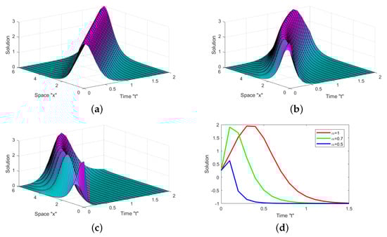
Figure 1. For Equation (21), (a–c) with parameters $k=-1,$$\xi$${}_1=1,$$\xi$${}_2=2,$$\xi$${}_3=-3,$$\xi$${}_4=2,$$\lambda =-3$,$x\in [0,6]$, $t\in [0,2],y=\omega =0.5,z=\frac{2}{3}$ displays the 3D representations and (d) displays the 2D plot for various values of $\alpha$ at $t=1.5$; there is no overlap between the curves of the solution. (a) $\alpha =1,\beta =0$(b)$\alpha =0.7,\beta =0.9$ and (c) $\alpha =0.5,\beta =0.9$.

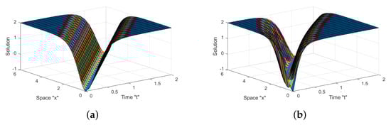
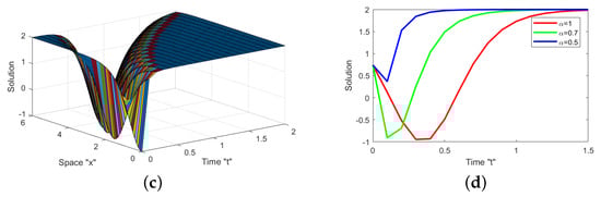
Figure 2. For Equation (26), (a–c) with parameters $k=1,$$\xi$${}_1=2,$$\xi$${}_2=$$\xi$${}_3=1,$$\xi$${}_4=-1,$$\lambda =-3.75$, $x\in [0,6]$, $t\in [0,2],y=z=0.5,\omega =1$ displays the 3D representations and (d) displays the 2D plot for various values of $\alpha$ at $t=2$; there is no overlap between the curves of the solution. (a) $\alpha =1,\beta =0$(b)$\alpha =0.7,\beta =0.9$ and (c) $\alpha =0.5,\beta =0.9$.

Figure 3. For Equation (39), (a–c) with parameters $m=0.5,$$\xi$${}_1=1,$$\xi$${}_2=2,$$\xi$${}_3=-1,$$\xi$${}_4=-1,$$\lambda =\frac{1}{2}(3-3\sqrt{13})$, $x\in [0,6]$, $t\in [0,2],y=\omega =z=1,$ displays the 3D representations and (d) displays the 2D plot for various values of $\alpha$ at $t=100$; there is no overlap between the curves of the solution. (a) $\alpha =1,\beta =0$(b)$\alpha =0.7,\beta =0.9$ and (c) $\alpha =0.5,\beta =0.9$.

6. Conclusions

In this study, we considered the (4+1)-dimensional fractional Fokas Equation (1) in the sense of the M-truncated derivative. By employing the extended tanhcoth and the Jacobi elliptic function method, we were able to achieve exact solutions. Furthermore, we generalized some earlier results for instance the results reported in [33,35,36]. The acquired solutions are essential in explaining a variety of fascinating and complex physical phenomena. Finally, the MATLAB tools was used to plot the Figure 1, Figure 2 and Figure 3 in order to show the effect of the fractional derivative on the analytical solution of the FFE (1).

References

- Oldham, K.B.; Spanier, J. The Fractional Calculus: Theory and Applications of Differentiation and Ntegration to Arbitrary Order, Vol. 11 of Mathematics in Science and Engineering; Academic Press: New York, NY, USA, 1974. [Google Scholar]
- Mohammed, W.W.; Bazighifan, O.; Al-Sawalha, M.M.; Almatroud, A.O.; Aly, E.S. The influence of noise on the exact solutions of the stochastic fractional-space chiral nonlinear schrödinger equation. Fractal Fract. 2021, 5, 262. [Google Scholar] [CrossRef]
- Podlubny, I. Fractional Differential Equations, Vol. 198 of Mathematics in Science and Engineering; Academic Press: San Diego, CA, USA, 1999. [Google Scholar]
- Hilfer, R. Applications of Fractional Calculus in Physics; World Scientific Publishing: Singapore, 2000. [Google Scholar]
- Oustaloup, A. La Commande CRONE: Commande Robuste d’Ordre Non Entier; Editions Hermès: Paris, France, 1991. [Google Scholar]
- Riesz, M. L’intégrale de Riemann-Liouville et le Problème de Cauchy pour L’équation des ondes. Bull. Société Mathématique Fr. 1939, 67, 153–170. [Google Scholar] [CrossRef]
- Wang, K.L.; Liu, S.Y. He’s fractional derivative and its application for fractional Fornberg-Whitham equation. Therm. Sci. 2016, 1, 54. [Google Scholar] [CrossRef]
- Miller, S.; Ross, B. An Introduction to the Fractional Calculus and Fractional Differential Equations; Wiley: New York, NY, USA, 1993. [Google Scholar]
- Caputo, M.; Fabrizio, M. A new definition of fractional differential without singular kernel. Prog. Fract. Differ. Appl. 2015, 1, 1–13. [Google Scholar]
- Atangana, A.; Baleanu, D. New fractional derivatives with non-local and non-singular kernel. Theory and application to heat transfer model. Therm. Sci. 2016, 20, 763–769. [Google Scholar] [CrossRef]
- Khalil, R.; Horani, M.A.; Yousef, A.; Sababheh, M. A new definition of fractional derivative. J. Comput. Appl. Math. 2014, 264, 65–70. [Google Scholar] [CrossRef]
- Atangana, A.; Baleanu, D.; Alsaedi, A. New properties of conformable derivative. Open Math. 2015, 13, 889–898. [Google Scholar] [CrossRef]
- Sousa, J.V.; de Oliveira, E.C. A new truncated Mfractional derivative type unifying some fractional derivative types with classical properties. Int. J. Anal. Appl. 2018, 16, 83–96. [Google Scholar]
- Yang, X.F.; Deng, Z.C.; Wei, Y. A Riccati-Bernoulli sub-ODE method for nonlinear partial differential equations and its application. Adv. Diff. Equ. 2015, 1, 117–133. [Google Scholar] [CrossRef]
- Mohammed, W.W.; Alshammari, M.; Cesarano, C.; El-Morshedy, M. Brownian Motion Effects on the Stabilization of Stochastic Solutions to Fractional Diffusion Equations with Polynomials. Mathematics 2022, 10, 1458. [Google Scholar] [CrossRef]
- Malfliet, W.; Hereman, W. The tanh method. I. Exact solutions of nonlinear evolution and wave equations. Phys. Scr. 1996, 54, 563–568. [Google Scholar] [CrossRef]
- Yan, Z.L. Abunbant families of Jacobi elliptic function solutions of the dimensional integrable Davey-Stewartson-type equation via a new method. Chaos Solitons Fractals 2003, 18, 299–309. [Google Scholar] [CrossRef]
- Hirota, R. Exact solution of the Korteweg-de Vries equation for multiple collisions of solitons. Phys. Rev. Lett. 1971, 27, 1192–1194. [Google Scholar] [CrossRef]
- Khan, K.; Akbar, M.A. The exp(-ψ(ς))-expansion method for finding travelling wave solutions of Vakhnenko-Parkes equation. Int. J. Dyn. Syst. Differ. Equ. 2014, 5, 72–83. [Google Scholar]
- Mohammed, W.W. Approximate solution of the Kuramoto-Shivashinsky equation on an unbounded domain. Chin. Ann. Math. Ser. B 2018, 39, 145–162. [Google Scholar] [CrossRef]
- Mohammed, W.W. Modulation Equation for the Stochastic Swift–Hohenberg Equation with Cubic and Quintic Nonlinearities on the Real Line. Mathematics 2020, 6, 1217. [Google Scholar] [CrossRef]
- Wazwaz, A.M. A sine-cosine method for handling nonlinear wave equations. Math. Comput. Model. 2004, 40, 499–508. [Google Scholar] [CrossRef]
- Yan, C. A simple transformation for nonlinear waves. Phys. Lett. A 1996, 224, 77–84. [Google Scholar] [CrossRef]
- Al-Askar, F.M.; Cesarano, C.; Mohammed, W.W. The analytical solutions of stochastic-fractional Drinfel’d-Sokolov-Wilson equations via (G′/G)-expansion method. Symmetry 2022, 14, 2105. [Google Scholar] [CrossRef]
- Zhang, H. New application of the (G′/G)-expansion method. Commun. Nonlinear Sci. Numer. Simul. 2009, 14, 3220–3225. [Google Scholar] [CrossRef]
- Zhang, Y.; Liu, X.; Belic, M.R.; Zhong, W.; Zhang, Y.; Xiao, M. Propagation dynamics of a light beam in a fractional Schrödinger equation. Phys. Rev. Lett. 2015, 115, 180403. [Google Scholar] [CrossRef] [PubMed]
- Zhang, Y.; Zhong, H.; Belic, M.R.; Zhu, Y.; Zhong, W.; Zhang, Y.; Christodoulides, D.N.; Xiao, M. PT symmetry in a fractional Schrödinger Equation. Laser Photonics Rev. 2016, 10, 526–531. [Google Scholar] [CrossRef]
- Mohammed, W.W.; Iqbal, N. Impact of the same degenerate additive noise on a coupled system of fractional space diffusion equations. Fractals 2022, 30, 2240033. [Google Scholar] [CrossRef]
- Fokas, A.S. Integrable nonlinear evolution partial differential equations in 4+2 and 3+1 dimensions. Phys. Rev. Lett. 2006, 96, 190210. [Google Scholar] [CrossRef]
- Ablowitz, M.J.; Clarkson, P.A. Solitons, Nonlinear Evolution Equations and Inverse Scattering; Cambridge University Press: New York, NY, USA, 1991. [Google Scholar]
- Davey, A.; Stewartson, K. On three-dimensional packets of surface waves. Proc. R. Soc. Lond. Ser. A Math. Phys. Eng. Sci. 1974, 338, 101–110. [Google Scholar]
- Zhang, S.; Chen, M. Painleve’ integrability and new exact solutions of the (4+1)-dimensional Fokas equation. Math. Probl. Eng. 2015, 2015, 367425. [Google Scholar] [CrossRef]
- He, Y. Exact solutions for (4+1)-dimensional nonlinear Fokas equation using extended F-expansion method and its variant. Math. Probl. Eng. 2014, 2014, 972519. [Google Scholar]
- Zhang, W.J.; Xia, T.C. Solitary wave, M-lump and localized interaction solutions to the (4+1)-dimensional Fokas equation. Phys. Scr. 2020, 95, 045217. [Google Scholar] [CrossRef]
- Al-Amr, M.O.; El-Ganaini, S. New exact traveling wave solutions of the (4+1)-dimensional Fokas equation. Comput. Math. Appl. 2017, 74, 1274–1287. [Google Scholar] [CrossRef]
- Kim, H.; Sakthivel, R. New exact traveling wave solutions of some nonlinear higher-dimensional physical models. Rep. Math. Phys. 2012, 70, 39–50. [Google Scholar] [CrossRef]
- Wazwaz, A.M. A variety of multiple-soliton solutions for the integrable (4+1)-dimensional Fokas equation. Waves Random Complex Media 2018, 31, 46–56. [Google Scholar] [CrossRef]
- Sarwar, S. New soliton wave structures of nonlinear (4+1)-dimensional Fokas dynamical model by using different methods. Alex. Eng. J. 2021, 60, 795–803. [Google Scholar] [CrossRef]
- Yang, Z.-Z.; Yan, Z.-Y. Symmetry groups and exact solutions of new (4+1)-dimensional fokas equation. Commun. Theor. Phys. 2009, 51, 876. [Google Scholar]
- Lu, C.N.; Hou, C.J.; Zhang, N. Analytical and numerical solutions for a kind of high-dimensional fractional order equation. Fractal Fract. 2022, 6, 338. [Google Scholar] [CrossRef]
- Ullah, N.; Asjad, M.I.; Awrejcewicz, J.; Muhammad, T.; Baleanu, D. On soliton solutions of fractional-order nonlinear model appears in physical sciences. AIMS Math. 2022, 7, 7421–7440. [Google Scholar] [CrossRef]
- Hussain, A.; Jhangeer, A.; Abbas, N.; Khan, I.; Sherif, E.-S.M. Optical solitons of fractional complex Ginzburg–Landau equation with conformable, beta, and M-truncated derivatives: A comparative study. Adv. Differ. Equ. 2020, 2020, 612. [Google Scholar] [CrossRef]
- Peng, Y.Z. Exact solutions for some nonlinear partial differential equations. Phys. Lett. A 2013, 314, 401–408. [Google Scholar] [CrossRef]
Disclaimer/Publisher’s Note: The statements, opinions and data contained in all publications are solely those of the individual author(s) and contributor(s) and not of MDPI and/or the editor(s). MDPI and/or the editor(s) disclaim responsibility for any injury to people or property resulting from any ideas, methods, instructions or products referred to in the content. |
© 2022 by the authors. Licensee MDPI, Basel, Switzerland. This article is an open access article distributed under the terms and conditions of the Creative Commons Attribution (CC BY) license (https://creativecommons.org/licenses/by/4.0/).