Abstract
For the first time, a novel concept of merging computational intelligence (the type-2 fuzzy system) and control theory (optimal control) for regulator and reference tracking in doubly fed induction generators (DFIGs) is proposed in this study. The goal of the control system is the reference tracking of torque and stator reactive power. In this case, the type-2 fuzzy controller is activated to enhance the performance of the optimum control. For instance, in abrupt changes of the reference signal or uncertainty in the parameters, the type-2 fuzzy system performs a complementary function. Both parametric uncertainty and a perturbation signal are used to challenge the control system in the simulation. The findings demonstrate that the presence of a type-2 fuzzy system as an additional controller or compensator significantly enhances the control system. The root mean square error of the suggested method’s threshold was 0.012, quite acceptable for a control system.
Keywords:
intelligent control; machine learning; type-2 fuzzy logic; fuzzy systems; stability analysis; adaptive control MSC:
93C42; 93C40; 68T05
1. Introduction
Among the different generators that are employed in modern wind-power-producing systems, doubly fed induction generators (DFIGs) have attracted maximum attention to themselves because of having advantages such as variable velocity action, the possibility of adjusting active and reactive power, and a low-cost transformer [,,,,]. Usually, double-feed generators have a back-to-back converter in the rotor circuit, which share the DC link. With proper control, these generators can be made to deliver power to the grid at ultra-synchronous speeds. Normally, the delivery power of these converters is between 25% and 30%. The extensive presence of wind turbines in modern power systems affects the dynamic behavior of the system and makes it more complex. This makes the use of advanced methods to control these systems more important. So far, many methods have been employed in relation to the control of DFIGs [,,,]. Generally, the control of the power elements in the DFIG rotor circuit is performed by proportional–integral (PI) robust controllers. However, the performance of the controlled system, despite these controllers, is not desirable due to the need for machine parameter values and power system dynamics to properly adjust their gains. Studies related to the stability analyses of the small signal of DFIG wind farms connected to the network have mainly considered a definitive approach to stability analyses, that for the oscillation nature of the wind, such analyses are very optimistic and will result in a particular operation point. For the stability analysis of such a system, Monte Carlo simulation methods in some studies have been proposed [,,,]. In [], an optimal multi-purpose PI controller with the directional evolution (DE) algorithm for DFIGs was proposed, where specific methods were used to apply limits and multi-objective optimization problems that increased the complexity of the controller design. To track the optimal power of the DFIG wind turbine system, a nonlinear controller with the sliding mode method was designed []. PI controllers play an important role in relation to DFIGs. However, to reach the power’s desired quality levels required in the new industry, new advanced methods are needed for controlling these generators. The reader is refereed to [] for more information on the methods utilized for controlling DFIG wind turbine systems.
In 1962, Pierson [] proposed the state-dependent Riccati equation (SDRE) method to approximate the solving of optimal control for nonlinear systems. The representation of a nonlinear system as a state-of-the-art linear system, called quasi-linearization, is the main idea of the SDRE method. After that, many methods based on quasi-linearization to solve various problems, such as filter design H∞, the designing of sliding mode suboptimal controllers for delayed systems, a retrograde design for delayed nonlinear systems, and others, have been developed [,,]. These methods have been used effectively in many practical fields, such as prescribing drugs for cancer and controlling the speed of permanent magnetic synchronous motors (PMSMs) [,]. One of the most attractive features of the SDRE method is that the designer can influence the performance of the system in a predicted way by adjusting the control and mode of the weight functions. For example, to speed up the response, we can increase the weight function related to the system modes, which will also result in an increase in control effort. At the same time, the designer, due to numerous state-dependent coefficient (SDC) displays for the nonlinear system, has a higher degree of freedom that can be used to improve the overall performance of the system. On the other hand, since the SDRE method system does not use any approximation in the system’s modeling, it keeps the nonlinear properties of the system, a crucial property, especially when the dynamics of the system are complex. In [], the SDRE method and its related theories are discussed. By developing type-1 fuzzy logic, we can achieve type-2 fuzzy logic. This system can be very useful for imprecision modeling. This system considers the uncertainty and vagueness of information. Type-2 fuzzy systems have better performance than type-1 fuzzy systems. The construction of the rules of this type of system is exactly like that of the type-1 system, and the only difference is the nature of the membership function. Each type-2 fuzzy membership function has one more parameter than that of type-1 fuzzy systems. This greatly helps because there are many membership functions in fuzzy systems, and therefore, there will be many adjustable parameters. Many adjustable parameters help to finetune the fuzzy system. Therefore, in this study, type-2 fuzzy systems were used [,,,,,].
According to the attractive features of SDRE controllers and the present nonlinear dynamics of DFIGs in modern power systems, in this study, we decided to use the SDRE controller to optimize the dynamic performance of these systems. For this purpose, all the necessary conditions for designing the optimal SDRE controller for a DFIG were investigated. In this paper, we used the SDRE method and increased the margin of the system’s stability by designing a stabilizer and simulations tracking the electromagnetic torque’s desired signals and the stator’s reactive power. Due to the presence of unknown parameters in the under-study system’s dynamics, the robustness of the resulting closed loop system was also investigated using the SDRE controller in the presence of an uncertainty in the system parameters. Moreover, a type-2 fuzzy system was used to improve the response of the control system. The results of the performed simulations in a MATLAB software environment indicated the improvement of the performance of system dynamics and the robustness of the designed controller function in the presence of uncertainty in the parameters for the different operation conditions of the system. At the same time, the analysis of specific values was performed to evaluate the effectiveness of the proposed method in improving the system’s stability margin.
The other parts of this paper are organized as follows: in the second part, the system, including the different parts of the DFIG wind turbine and its state space model, are introduced. The third section examines the SDRE controller, which needs steps for designing, and its sustainability theories. In this next section, the various steps that were required for designing the stabilizer and tracker with the SDRE method are separately described. The type-2 fuzzy system is described in the fourth section. In the fifth section, the results of the performed simulations in the MATLAB software environment, along with their analyses, are provided. Finally, the sixth section is allotted to the conclusion of the paper.
2. DFIG Mathematical Model
In this section, equations related to the DFIG for use in the other parts of the paper are investigating. For the stability of power system studies, the generator was modeled as a transient reactance-backed voltage source. The system’s diagram is shown in Figure 1. Differential equations of the rotor and stator circuits of the induced generator in the d-q source frame are as follows:
where is the self-inductance of the stator, is the self-inductance of the rotor, is the mutual inductance, is the rotor resistance, is the stator reactance, is the time constant of the rotor circuit, is the transient reactance of the stator, is the angular velocity of the rotor, and are the voltages related to the transient reactance of the stator along the d and q axes, is the rotor voltage along the d axis, is the rotor voltage along the q axis, and are the stator currents along with the d and q axes, respectively, and and (t) are the voltages corresponding with these currents. All symbols used along with their explanations are listed in Table A1 in Appendix A.
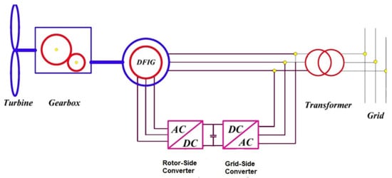
Figure 1.
Wind turbine diagram with the DFIG.
The wind turbine drive includes turbines, gearboxes, axles, and other mechanical components. In sustainability studies of the power system, the use of a dual-mode model for the turbine drive has been very important. Therefore, the wind turbine shaft was relatively softer than the shaft used in conventional power plants. The equations related to the two-mass model of the wind turbine drive are as follows:
where and are the turbine velocity and dual-axis angle, respectively, and and are the turbine and generator inertia constants, respectively. The equations of (or electromagnetic torque) and (or axis torque) are as follows:
where is the axis hardness coefficient, is its damping coefficient, and is the mechanical torque that is the input of the wind turbine power’s assumed constant. By considering Equations (1) to (4), a space mode model of the wind turbine DFIG is obtained as follows:
where is the system state variable vector and is the vector of the control input.
3. SDRE Nonlinear Sub-Optimal Controller
According to the very interesting properties of the SDRE control and nonlinear dynamics of the DFIG wind turbine, in this part, the SDRE method and different stages are separately stated for two control purposes: the stabilizer design and tracker. According to the commonality of both methods in quasi-linear discussions, first, this topic is stated in Section 3.1, Section 3.2 and Section 3.3, and then the requirements and necessary steps for the control design are separately given to meet each of the objectives above with the SDRE method.
3.1. Quasi-Linearization
Consider the following nonlinear system:
where and , and is the initial condition. At first glance, the quasi-linearization process seems very simple. In the way that a factorization as is performed, , which is a functional matrix. The important point in this factorization is the existence of different structures for the decomposition of as a fraction of . For example, when is and , any linear combination of and constructs another quasi-linear structure as
where is a known function of . In the case of non-scalar systems, there are an infinite number of ways to form the state matrix , which is the advantage of the SDRE method, providing the designer with an additional degree of freedom.
3.2. Designing of Stabilizer with SDRE Method
The design of a stabilizer functions to make all the states in a system zero. In this case, we used an unlimited horizon SDRE controller, in which its target was reset to zero for all the states, minimizing the following cost function:
where and are the weight matrices, depending on the state, and are positive definite and semi-definite positive, respectively. The main step in designing an SDRE controller is solving the following equation:
After solving this equation, the optimal control law, which minimizes the second-order cost defined in Equation (6), results in:
It is important to note that Equation (7) has a definite symmetric positive solution of if and only if and are point-to-point controllable and point-to-point visible, respectively. The point-to-point controllability of and point-to-point visibility of are also met if the point-to-point controllability and visibility matrices are in full order, respectively:
Because of the infinite display of the SDC for the matrix, the designer meets the requirements above with more freedom of choice in selecting the appropriate SDC display.
3.3. SDRE Optimal Tracker Controller Design
To track a desired path, the tracker controller was designed by the desired output signal in such a way that the output signal must follow the desired path with the presence of the designed controller. Consider the following nonlinear system:
where is the state vector of the system, is the input vector of the control, and . The output vector of the system and functions are , , and . Below, we used the methods of [,] to design the tracker controller with the SDRE method. The problem of non-linear optimal tracking of an unlimited horizon with a discounted cost function is to find the control function of , so that the output of the system tracks the desired path of and the following cost function is minimized:
where is the discount agent of , and Rq*q are the definite positive and semi-definite positive symmetric matrices, respectively. Assume that the desired path has the following equations:
where and are the state vector and output related to the desired path, respectively, and 0, are the functions. Based on the quasi-linearization idea, to solve the above problem, first write the quasi-linear forms of the function , as
where the functions are , , , and . By the definition of U(t) = , , the cost function of (7) changes to the below form:
Then the dynamic of the new state variable of is
Now, according to Equations (9), (11), and (12), the dynamics of the quasi-linearization of the state vector will be:
where and 0 are the uniform and zero matrices with the proper dimensions, respectively. Therefore, the problem of the nonlinear optimal configuration of unlimited horizons described by Equations (13) and (14) should be solved instead of the existing tracking problem. Finally, the optimal control law for the considered tracking problem proceeds as follows:
where the matrix is the definite solution of the positive symmetric of the Riccati equation:
In this study, to improve the response of the control system, the type-2 fuzzy system produced a compensating signal () in parallel with the main (optimal) controller. Therefore, the total control signal is expressed as Equation (15):
In the following, the details of the type-2 fuzzy system are described.
4. Type-2 Fuzzy System
In this study, a fuzzy controller was responsible for generating the compensating control signal. The presence of uncertainty and sudden changes in the reference signal further emphasized the role of the compensatory signal. Figure 2 shows the structure of the proposed type-2 fuzzy system. Type-2 fuzzy systems have better efficiency in noisy environments because the membership in this type of fuzzy system are fuzzy numbers, not certain values []. Wu in [] showed that, given the same rule base, type-1 fuzzy systems cannot perform the complex control surfaces that type-2 fuzzy systems can.
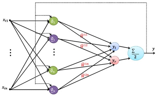
Figure 2.
The structure of the proposed type-2 fuzzy neural network.
The calculations of the first layer are given as follows:
where and are the upper and lower of the jth input and neuron, respectively. Therefore, the first-layer outputs are calculated as follows:
where and are the upper and lower of the neuron , respectively. Moreover, is the input vector, and is the center of all neurons. The second layer’s left and right endpoints are as follows:
where and are the left and right switching points, respectively, which can be calculated using the trial-and-error method or the Karnik–Mendel (KM) algorithm [,]. Moreover, , , , and are the mean value of the first-layer neurons, weights, center of weights, and spread of weights, respectively. Finally, the network general output can be calculated as follows:
The gradient descent method was used to teach the network. As shown in Figure 3, the optimal controller generated control signals by receiving the system states as well as the reference values of reactive power and electrical torque. On the other hand, the input of the fuzzy controller was system states, and the error rate (reactive power and electrical torque) was used to update the controller parameters. Naturally, sudden changes in the reference signal led to a large error, and therefore, the fuzzy controller parameters were quickly updated and in proportion to the error rate. This made the control system faster and more accurate.
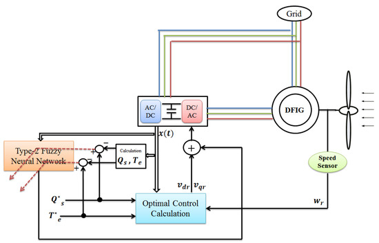
Figure 3.
The proposed control system for DFIG.
Remark.
In this study, type-2 systems were used to estimate DFIG uncertainties. For future studies, the suggested controller can be improved using new stable adaptations [], optimization schemes [], neural networks [], and new machine learning techniques [,].
5. Simulation Results
In Section 5.1, the results of the simulations in MATLAB software are provided to design the SDRE controller for the improvement of the system stability of the DFIG wind turbine. The simulations were performed for different work conditions of systems, including different velocities of wind. In all the simulations, the optimal control alone (without the compensator) was compared with the optimal control method with the compensator based on the type-2 fuzzy system. In Section 5.2, the results of the SDRE sub-optimal tracker controller design for tracking the desired signals of reactive power, stator power, and the DFIG’s electromagnetic torque are presented. For solar power systems integrated into the DFIG, the proposed method can be efficient. Of course, in this case, the mathematical equations of the system will change.
5.1. Design of Stabilizer for DFIG
As seen from Equations (1)–(4), a wind turbine system with a DFIG is a nonlinear system. The model that was used for designing in this section was the seven-order model with a two-control input according to Equations (1)–(4). For designing the controller with the SDRE method, first was chosen in such a way that even if the system was not fully point-controllable, the pair’s point stability condition of was met. After determining the appropriate SDC display, the weight matrices of R and Q were determined to design the desired controller. We used the matrices of and to design the control, shown as follows:
Although there were several ways to select the matrix among the infinite possible SDC displays, only one of them will lead to the optimal performance of the closed loop system, the detection of which is very difficult. As a result, the only condition for selecting was that the relation of was established. The results related to the performed simulations in the presence of optimal control with and without a type-2 fuzzy compensator controller are given in Figure 2. Figure 4a–d are related to the current signals of the stator and its transient voltage along the q and d vectors. It is assumed that a disturbance was applied to the system in . As can be seen, the result signals of the optimal controller (with and without a type-2 fuzzy compensator) by damping the created oscillations were adjusted to their desired equilibrium points. Figure 5a,b are also related to the and control signals produced by the mentioned controllers, respectively.
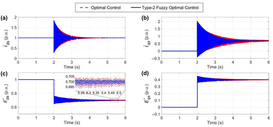
Figure 4.
The shapes of (a–d) are related to the stator current signals and and their transient voltages , and , respectively. Note that “p.u.” means per unit.
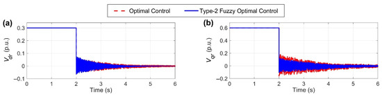
Figure 5.
The shapes of (a,b) are related to the rotor voltage signals along with the d and q vectors as control signals, respectively. Before the moment , the system is in its stable state, and at , disturbance enters the system.
To challenge the proposed control system, it was assumed that a three-phase-to-ground fault was applied at , and within 0.1 s, the breaker worked. Figure 6 shows the optimal control system performance (with and without a type-2 fuzzy system) without any control system. In Figure 6a, at , a three-phase-to-ground fault had occurred. In fact, by applying this fault, the performance of the control system was challenged. The fault was assumed to last for 0.1 s and ended at . Reaching 0.5 p.u. was the saturation limit of the system, assumed to be fixed there in the simulation.
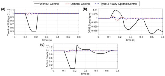
Figure 6.
(a) Terminal voltage in three-phase-to-ground fault, (b) DFIG speed in three-phase-to-ground fault, and (c) active power in three-phase-to-ground fault.
As can be seen from Figure 6, the results without a control system were not defensible. It can be carefully observed in the figure that the presence of a type-2 fuzzy compensator in the optimal control system made the signals smoother and provided a more appropriate response.
5.2. Tracker Controller Design for DFIG
The model used to design the tracker controller using the SDRE method to track the desired signals of electromagnetic torque and the reactive power of the stator is in the form of the following equations:
The rotor speed, stator current, and rotor current are considered as the state variables. The output matrix C is a single-order matrix of the fifth order, and the matrices , , , and are as follows:
where is the stator self-inductance, is the rotor self-inductance, is the inertial moment, and is the number of poles, . The variables , , , and in the relation are defined as
The outputs to be tracked by the designed controller were the electromagnetic torque signals and reactor power of the reactor, which must track the time-varying reference signals using the designed controller. The reactor power of the reactor was controlled in the stator terminal to keep the value of the electric power factor constant (). The present relationships for the electromagnetic torque and stator reactor power are as follows:
Related signals to the stator reactive power and electromagnetic torque of the DFIG with the electrical power coefficient () are in relation as
Note that in practice, by controlling one of the two signals or , the tracking operation of the desired values was performed. By forming the system controllability matrix as follows, the point controllability of the pair and was examined:
where to are the columns of the obtained control point matrix. By finding a quadratic order of five from the matrix , which has non-volatile determinants, it can be concluded that has a complete rank, and the system was completely point-controllable. With the formation of a minor from the first five columns of the matrix to check the point control of the pair , the resulting matrix determinants were calculated:
where , , and . The determinant of the above matrix () is equal to . According to the definition of and and according to the values of their equilibrium points, we can ignore the sentence versus the sentence . As a result, the matrix determinant is equal to . Given the equilibrium points, we concluded that these determinants have a non-zero value. Therefore, the considered pair is point-to-point controllable. Similarly, by forming the point visibility matrix, we could examine the visibility of . It can be shown that this condition was established in relation to the SDC display used, denied due to the high volume of calculations.
The results of the simulations are shown in Figure 7. As seen in the waveform, the stator reactive power and electromagnetic torque were well-traced to their reference values. Therefore, the tracking operation was performed with good speed and by damping the fluctuations caused by the change in the reference signal. In fact, tracking the optimum signal strength of the reactor power indicated that the power factor coefficient remained constant. The simulations were performed under the conditions that the desired values for the and signals were changed as follows.
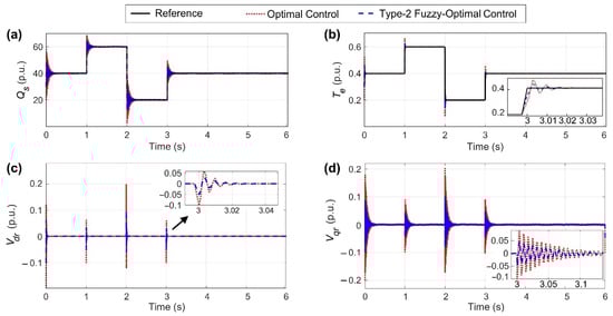
Figure 7.
The shapes of (a–d) are related to the stator reactive power and electromagnetic torque tracking performance and created control signals by optimal control (with and without the type-2 fuzzy system).
First, (Newton meter), and . In , the desired values were changed to and . In , the reference values were and . In , the desired values were changed to and .
In the following, the performance of the control system was challenged by applying parametric indeterminacy. First, the system parameters were reduced by 20% at . The performance of optimal control (with and without the type-2 fuzzy system) and the system without control is illustrated in Figure 8.
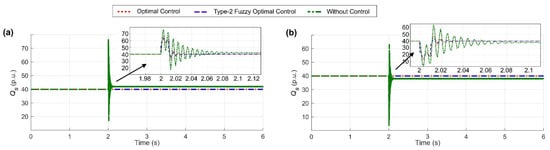
Figure 8.
Control system operation (with and without type-2 fuzzy system) and without controller to (a) decrease and (b) increase DFIG parameters by 20%.
As shown in Figure 8, the sudden decrease or increase of DFIG parameters (as much as 20%) was well-managed by the optimal control system (with and without the type-2 fuzzy system), and after about 0.03 s, the system returned to its stable mode. However, the system without a controller, in addition to many overshoots, suffered from a steady-state error. The reason that the system did not diverge (unstable) without a controller was that there were saturating elements and limiters in the system.
The root mean square error (RMSE) and mean absolute error (MAE) are two popular statistical metrics used to evaluate the performance of models. They are defined as
where are the number of observations, and the actual and predicted values, respectively. To better evaluate the proposed method, the methods of [,] were implemented, and the RMSE and MAE were calculated for them. Table 1 shows the RMSEs of four control methods, including optimal control, active control [], a fractional order PI controller [], and the proposed method for both the case without uncertainty and that for the presence of parametric uncertainty.

Table 1.
Comparison of control methods based on the RMSE criterion.
As can be seen in Table 1, the proposed method was superior to other methods by a large margin. The reason for this may be the simultaneous use of optimal control capabilities and the type-2 fuzzy system. Moreover, we can improve this study by using a type-3 fuzzy system. For more information about this method, refer to [].
6. Conclusions
In this paper, the type-2 fuzzy system was used to compensate for the optimal control of a DFIG. Type-2 fuzzy systems with more adjustable parameters than traditional type-1 fuzzy systems can control the system better and more accurately. The nonlinear and sub-optimal SDRE method was used in the optimal control section. The proposed method was employed for the system’s stability margin improvement and simultaneous tracking of the desired signals of electromagnetic torque and stator reactive power. The proposed weights of the type-2 fuzzy system, in addition to the membership functions, led to an increase in the parameters of the control system (increasing the degree of freedom); therefore, the control system became more precise. The RMSE for the proposed method was 0.012, which was significantly lower than that of other control methods. As suggestions for further work, the type-3 fuzzy system can be used to compensate for the control signal. Type-3 fuzzy systems have more control parameters than type-2 fuzzy systems and have a higher degree of freedom, so we can perform more control actions on the system and obtain better results. Structural and parametric uncertainties can also be considered for the DFIG model, further challenging the control system.
Author Contributions
Conceptualization, L.X., G.C., T.W., Y.G., A.M. and E.G.; methodology, L.X., G.C., T.W., Y.G., A.M. and E.G.; Formal analysis, L.X., G.C., T.W., Y.G., A.M. and E.G.; Writing—original draft preparation, L.X., G.C., T.W., Y.G., A.M. and E.G. All authors have read and agreed to the published version of the manuscript.
Funding
The paper is supported by Zhejiang Key Laboratory of Parts Rolling Technology (no. PR-22002), the general scientific research projects of the Zhejiang Provincial Department of Education (no. A-0275-21-059) and Key Research and Development Program of Zhejiang Province (no. 2022C01147).
Institutional Review Board Statement
Not applicable.
Informed Consent Statement
Not applicable.
Data Availability Statement
The paper presents no data.
Conflicts of Interest
The authors declare no conflict of interest.
Appendix A
Table A1.
Nomenclature.
Table A1.
Nomenclature.
| Symbol | Description |
|---|---|
| Self-inductance of stator | |
| Self-inductance of rotor | |
| Mutual inductance | |
| Rr | Rotor resistance |
| Xs | Stator reactance |
| Time constant of the rotor circuit | |
| Angular velocity of the rotor | |
| Voltages related to the transient reactance of the stator along the d axis | |
| Voltages related to the transient reactance of the stator along the q axis | |
| Rotor voltage along the d axis | |
| Rotor voltage along the q axis | |
| Stator current along with the d axis | |
| Stator current along with the q axis | |
| Turbine velocity | |
| Dual-axis angle | |
| Axis hardness coefficient | |
| Damping coefficient | |
| Tm | Mechanical torque |
| Value of the first layer neurons | |
| Weights | |
| The center of the weights | |
| The spread of the weights |
References
- Murillo-Yarce, D.; Riffo, S.; Restrepo, C.; González-Castaño, C.; Garcés, A. Model Predictive Control for Stabilization of DC Microgrids in Island Mode Operation. Mathematics 2022, 10, 3384. [Google Scholar] [CrossRef]
- Sadiq, M.; Aragon, C.A.; Terriche, Y.; Ali, S.W.; Su, C.-L.; Buzna, Ľ.; Elsisi, M.; Lee, C.-H. Continuous-Control-Set Model Predictive Control for Three-Level DC–DC Converter with Unbalanced Loads in Bipolar Electric Vehicle Charging Stations. Mathematics 2022, 10, 3444. [Google Scholar] [CrossRef]
- Mohammadi, F.; Mohammadi-ivatloo, B.; Gharehpetian, G.B.; Ali, M.H.; Wei, W.; Erdinç, O.; Shirkhani, M. Robust Control Strategies for Microgrids: A Review. IEEE Syst. J. 2021, 16, 2401–2412. [Google Scholar] [CrossRef]
- Iranmehr, H.; Aazami, R.; Tavoosi, J.; Shirkhani, M.; Azizi, A.; Mohammadzadeh, A.; Mosavi, A.H. Modeling the Price of Emergency Power Transmission Lines in The Reserve Market Due to The Influence of Renewable Resources. Front. Energy Res. 2022, 9, 792418. [Google Scholar] [CrossRef]
- Danyali, S.; Aghaei, O.; Shirkhani, M.; Aazami, R.; Tavoosi, J.; Mohammadzadeh, A.; Mosavi, A. A New Model Predictive Control Method for Buck-Boost Inverter-Based Photovoltaic Systems. Sustainability 2022, 14, 11731. [Google Scholar] [CrossRef]
- Aazami, R.; Heydari, O.; Tavoosi, J.; Shirkhani, M.; Mohammadzadeh, A.; Mosavi, A. Optimal Control of an Energy-Storage System in a Microgrid for Reducing Wind-Power Fluctuations. Sustainability 2022, 14, 6183. [Google Scholar] [CrossRef]
- Taghieh, A.; Mohammadzadeh, A.; Zhang, C.; Kausar,, N.; Castillo, O. A type-3 fuzzy control for current sharing and voltage balancing in microgrids. Appl. Soft Comput. 2022, 129, 109636. [Google Scholar] [CrossRef]
- Li, P.; Hu, W.; Hu, R.; Huang, Q.; Yao, J.; Chen, Z. Strategy for wind power plant contribution to frequency control under variable wind speed. Renew. Energy 2019, 130, 1226–1236. [Google Scholar] [CrossRef]
- Chaudhuri, A.; Datta, R.; Kumar, M.P.; Davim, J.P.; Pramanik, S. Energy Conversion Strategies for Wind Energy System: Electrical, Mechanical and Material Aspects. Materials 2022, 15, 1232. [Google Scholar] [CrossRef]
- Chen, F.; Qiu, X.; Alattas, K.A.; Mohammadzadeh, A.; Ghaderpour, E. A New Fuzzy Robust Control for Linear Parameter-Varying Systems. Mathematics 2022, 10, 3319. [Google Scholar] [CrossRef]
- Tavoosi, J.; Shirkhani, M.; Abdali, A.; Mohammadzadeh, A.; Nazari, M.; Mobayen, S.; Asad, J.H.; Bartoszewicz, A. A New General Type-2 Fuzzy Predictive Scheme for PID Tuning. Appl. Sci. 2021, 11, 10392. [Google Scholar] [CrossRef]
- Tian, S.; Li, Z.; Li, H.; Hu, Y.; Lu, M. Active control method for torsional vibration of DFIG drive chain under asymmetric power grid fault. IEEE Access 2020, 8, 155611–155618. [Google Scholar] [CrossRef]
- Riaz, A.; Kousar, S.; Kausar, N.; Pamucar, D.; Addis, G.M. Codes over Lattice-Valued Intuitionistic Fuzzy Set Type-3 with Application to the Complex DNA Analysis. Complexity 2022, 2022, 5288187. [Google Scholar] [CrossRef]
- Hemmati, R.; Faraji, H.; Beigvand, N.Y. Multi objective control scheme on DFIG wind turbine integrated with energy storage system and FACTS devices: Steady-state and transient operation improvement. Int. J. Electr. Power Energy Syst. 2022, 135, 107519. [Google Scholar] [CrossRef]
- Yang, B.; Yu, T.; Shu, H.; Dong, J.; Jiang, L. Robust sliding-mode control of wind energy conversion systems for optimal power extraction via nonlinear perturbation observers. Appl. Energy 2018, 210, 711–723. [Google Scholar] [CrossRef]
- Mahvash, H.; Taher, S.A.; Rahimi, M.; Shahidehpour, M. Enhancement of DFIG performance at high wind speed using fractional order PI controller in pitch compensation loop. Int. J. Electr. Power Energy Syst. 2019, 104, 259–268. [Google Scholar] [CrossRef]
- Nekoo, S.R. Tutorial and review on the state-dependent Riccati equation. J. Appl. Nonlinear Dyn. 2019, 8, 109–166. [Google Scholar] [CrossRef]
- Qin, B.; Sun, H.; Ma, J.; Li, W.; Ding, T.; Wang, Z.; Zomaya, A.Y. Robust H∞ Control of Doubly Fed Wind Generator via State-Dependent Riccati Equation Technique. IEEE Trans. Power Syst. 2018, 34, 2390–2400. [Google Scholar] [CrossRef]
- Sharafian, A.; Fard, Z.E. State-dependent Riccati equation sliding mode observer for mathematical dynamic model of chronic myelogenous leukaemia. Int. J. Eng. Syst. Model. Simul. 2018, 10, 75–86. [Google Scholar] [CrossRef]
- Huang, N.; Chen, Q.; Cai, G.; Xu, D.; Zhang, L.; Zhao, W. Fault Diagnosis of Bearing in Wind Turbine Gearbox Under Actual Operating Conditions Driven by Limited Data with Noise Labels. IEEE Trans. Instrum. Meas. 2021, 70, 1–10. [Google Scholar] [CrossRef]
- Babaei, N.; Salamci, M.U. Mixed therapy in cancer treatment for personalized drug administration using model reference adaptive control. Eur. J. Control. 2019, 50, 117–137. [Google Scholar] [CrossRef]
- Rafaq, M.S.; Nguyen, A.T.; Choi, H.H.; Jung, J.W. A robust high-order disturbance observer design for SDRE-based suboptimal speed controller of interior PMSM drives. IEEE Access 2019, 7, 165671–165683. [Google Scholar] [CrossRef]
- Lin, L.G.; Xin, M. Computational enhancement of the SDRE scheme: General theory and robotic control system. IEEE Trans. Robot. 2020, 36, 875–893. [Google Scholar] [CrossRef]
- Mendel, J.; Hagras, H.; Tan, W.W.; Melek, W.W.; Ying, H. Introduction to Type-2 Fuzzy Logic Control: Theory and Applications; John Wiley & Sons: Hoboken, NJ, USA, 2014. [Google Scholar] [CrossRef]
- Karnik, N.N.; Mendel, J.M. Centroid of a type-2 fuzzy set. Inf. Sci. 2001, 132, 195–220. [Google Scholar] [CrossRef]
- Wu, D.; Mendel, J.M. Enhanced Karnik--Mendel Algorithms. IEEE Trans. Fuzzy Syst. 2009, 17, 923–934. [Google Scholar]
- Mittal, K.; Jain, A.; Vaisla, K.S.; Castillo, O.; Kacprzyk, J. A comprehensive review on type 2 fuzzy logic applications: Past, present, and future. Eng. Appl. Artif. Intell. 2020, 95, 103916. [Google Scholar] [CrossRef]
- Duran, K.; Bernal, H.; Melgarejo, M. Improved iterative algorithm for computing the generalized centroid of an interval type-2 fuzzy set. In Proceedings of the NAFIPS 2008—2008 Annual Meeting of the North American Fuzzy Information Processing Society, New York, NY, USA, 19–22 May 2008; pp. 1–5. [Google Scholar]
- Guo, X.; Shirkhani, M.; Ahmed, E.M. Machine-Learning-Based Improved Smith Predictive Control for MIMO Processes. Mathematics 2022, 10, 3696. [Google Scholar] [CrossRef]
- Wu, D. On the fundamental differences between interval type-2 and type-1 fuzzy logic controllers. IEEE Trans. Fuzzy Syst. 2012, 20, 832–848. [Google Scholar] [CrossRef]
- Li, D.; Yu, H.; Tee, K.P.; Wu, Y.; Ge, S.S.; Lee, T.H. On Time-Synchronized Stability and Control. IEEE Trans. Syst. Man Cybern. Syst. 2022, 52, 2450–2463. [Google Scholar] [CrossRef]
- Xu, X.; Lin, Z.; Li, X.; Shang, C.; Shen, Q. Multi-objective robust optimisation model for MDVRPLS in refined oil distribution. Int. J. Prod. Res. 2022, 60, 6772–6792. [Google Scholar] [CrossRef]
- Zheng, W.; Tian, X.; Yang, B.; Liu, S.; Ding, Y.; Tian, J.; Yin, L. A Few Shot Classification Methods Based on Multiscale Relational Networks. Appl. Sci. 2022, 12, 4059. [Google Scholar] [CrossRef]
- Zheng, W.; Zhou, Y.; Liu, S.; Tian, J.; Yang, B.; Yin, L. A Deep Fusion Matching Network Semantic Reasoning Model. Appl. Sci. 2022, 12, 3416. [Google Scholar] [CrossRef]
- Dang, W.; Guo, J.; Liu, M.; Liu, S.; Yang, B.; Yin, L.; Zheng, W. A Semi-Supervised Extreme Learning Machine Algorithm Based on the New Weighted Kernel for Machine Smell. Appl. Sci. 2022, 12, 9213. [Google Scholar] [CrossRef]
- Castillo, O.; Castro, J.R.; Melin, P. Interval Type-3 Fuzzy Systems: Theory and Design. Studies in Fuzziness and Soft Computing; Springer: Cham, Switzerland, 2022; Volume 418. [Google Scholar] [CrossRef]
Disclaimer/Publisher’s Note: The statements, opinions and data contained in all publications are solely those of the individual author(s) and contributor(s) and not of MDPI and/or the editor(s). MDPI and/or the editor(s) disclaim responsibility for any injury to people or property resulting from any ideas, methods, instructions or products referred to in the content. |
© 2022 by the authors. Licensee MDPI, Basel, Switzerland. This article is an open access article distributed under the terms and conditions of the Creative Commons Attribution (CC BY) license (https://creativecommons.org/licenses/by/4.0/).