Dynamic Model of Enterprise Revenue Management Based on the SFA Model

Abstract

The actual problem of enterprise revenue management that requires an effective solution is considered. Revenue is the main source of cash proceeds specifically from the main enterprise activities, as well as one of the main factors affecting enterprise functioning. As a result, the amount of revenue is extremely important for the company—it must be sufficient to ensure the repayment of all expenses of the company and the formation of the required profit amount. However, the amount of revenue itself is not the only important characteristic of revenue; the revenue stability over time and the revenue receipt regularity are no less important. The purpose of this work is to develop a dynamic model of enterprise revenue management, which differs from the model known in the literature by considering the parameter of enterprise performance efficiency. The parametric method of Stochastic Frontier Analysis (SFA) is used as a method to evaluate the efficiency of an enterprise. Financial indicators are used as input and output data. The model was tested on six small business sectors of a single-industry town for the period from 2007 to 2021. Data collection was carried out using the SPARK system, which allows selecting enterprises for research by the status of the enterprise (bankrupt/operating), by the size of the enterprise (large/medium/small/micro), etc. The above calculations based on the constructed modified model have demonstrated the possibility of using the enterprise’s revenue management with the desired rate of change and with the work efficiency parameter.

1. Introduction

The financial stability of an organization is usually assessed from the standpoint of a long-term perspective by a system of indicators, which includes several main sections: Assessment of property status; liquidity assessment; assessment of financial stability; assessment of business activity; profitability assessment. Each group has between 6 and 12 different coefficients (41 in total) [1,2].

In addition to coefficient analysis, a number of classification models that separate bankrupt firms from stable borrowers and predict the possible bankruptcy of a borrowing firm were used.

There are numerous proprietary methods to assess the probability of bankruptcy, which operate on a wide range of indicators. Such factor models were developed using multivariate (multiplicative) discriminant analysis.

The most well-known models for assessing the bankruptcy probability are:

• Altman models [3,4,5];
• The four-factor Lis’ model, which is appropriate for Russian enterprises with such organizational and legal forms as joint-stock companies [6,7];
• Fulmer’s model—a nine-factor model for assessing bankruptcy risk [8];
• Springate’s model to predict enterprise bankruptcy [9,10];
• Taffler’s four-factor bankruptcy model [11];
• Saifullin–Kadykov’s model of enterprises bankruptcy is a medium-term rating model for predicting bankruptcy risk, developed by Russian scientists, which can be applied to any industry and enterprises of various sizes [12,13]; it should be noted that these models’ bankruptcy forecasting differs between countries, sectors of the economy, enterprise size or age;
• In addition to these models, the models of G.V. Davydova and A.Iu. Belikov [14], O.P. Zaitseva [15], A.H. Makareva and L.V. Andreeva [16], and others should be also specified.

The analysis of the models showed that there is no universal model to assess enterprise bankruptcy. The applicability limits of the models are related to the economic conditions under which the models were obtained. It was shown that foreign models are not very appropriate for Russian conditions [17]. In addition, the financial stability models of enterprises in various industries can also differ significantly from each other. In this regard, for enterprises of various sectors, the author’s models for assessing the enterprise revenue, as the most significant indicator associated with financial stability, were built in the works [7,18].

Building a model for assessing the financial stability of enterprises can be viewed as a direct task. To manage the bankruptcy risk, the inverse problem—how to change the financial indicators so that the key indicator takes the given values—should be considered [19]. In this work, a dynamic model for managing a key indicator, i.e., the enterprise revenue, was built, considering the efficiency of the enterprise’s activities, based on the SFA model [20,21,22,23].

The SFA method is used in various types of economic activity, which are reviewed in a number of works [24,25,26,27,28,29,30,31,32,33,34,35,36,37,38], etc. For the first time, the authors [25,26] use the method to estimate the inefficiency of every enterprise and then include it as a covariance in the Cox proportional failure rates model, the Weibull survival model, and the early warning model, respectively. Then the authors [27] propose the one-step approach to assess the impact of inefficiency on the time before a US commercial banks bankruptcy, which will allow the calculation of the marginal distribution of inefficiency for every observed unit and facilitate the statistical inference of non-linear parameter functions, such as returns to scale. However, the study was only conducted on cross-sectional data and not on panel data.

Researchers [28] propose a semiparametric SFA model for the banking industry in Indonesia from 2000 to 2015. The work [29] uses the SFA model to estimate two bankruptcy probability indicators based on the Merton model [30] and the discrete-time risk model [31] of credit institutions. Other authors [32] consider the compatibility of quantile regression with the SFA method and propose ways to overcome conflicts between them, also they develop tools for applied efficiency analysis using quantile methods in the SFA models context.

In another work [32], the authors studied the impact of the technical efficiency level on the risks of financial stability loss by industrial organizations of the Russian Federation; the authors [33] studied the Australian fisheries sector; work [34] is devoted to the analysis of the effectiveness of individual transport units in military logistics and military vehicles in carrying out the tasks of transporting goods for supply and special needs of military institutions; the authors [35] conducted an econometric analysis of a Swedish secondary school’s efficiency, the obtained results allow judging a relatively limited distribution of school inefficiency indicators; work [36] considers the efficiency of agricultural production; work [37] is devoted to the software development and pharmaceutical industry; the authors [23] consider enterprises that produce concrete and cement in accordance with OKVED (Russian National Classifier of Economic Activities).

In this paper, branches of economic activity are considered.

2. Materials and Methods: Model

Let us suppose that we have identified n indicators that are the most critical for assessing the bankruptcy risk, affecting the proceeds from sales of products, as the main source of financial resources formation of the enterprise. Assume the values of these indicators go beyond the lower acceptable limits, and we want to increase their values in order to avoid bankruptcy. To do this, investments in the enterprise are needed.

Let us denote $x_{ji}\left(t\right)$, j = 1,…,n; i = 1,…,m for the financial performance of the j-th enterprise at the time t (t = 0,…,T−1), where n—the number of enterprises; T—the planned time point for the enterprise to exit the critical state; $x_i^0\left(t\right)$—planned values of indicators corresponding to the sustainable functioning of the enterprise; $V_j\left(t\right)$—proceeds from the sale of the j-th enterprise products, required to bring the enterprise out of the crisis (in fact, this involves the additional investment in the enterprise necessary to overcome the crisis); $V^0\left(t\right)$—planned revenue necessary for sustainable enterprise functioning. It is assumed that part of these proceeds is invested in production.

Let us represent the dependence of the revenue of the j-th enterprise on time in the form of multiple regression

$$V_j\left(t\right)={{\displaystyle \sum }}_{i=1}^m{a}_i\left(t\right)·x_{ji}\left(t\right),$$

(1)

where $a_i$—the regression coefficients.

We represent the dependence of the planned revenue in the form

$$V_j^0\left(t+1\right)=\left(1+{\mu }_j^0\left(t\right)\right)V_j^0\left(t\right),$$

(2)

where ${\mu }_j^0\left(t\right)$—the desired growth rate of revenue of the j-th enterprise. The revenue growth rate should be such that the planned revenue at least covers inflation.

We represent the dependence of the financial indicator $x_{ji}\left(t\right)$ on time in the form

$$x_{ji}\left(t+1\right)=\left(x_{ji}\left(t\right)+u_{ji}\left(t\right)\right),i=1,\dots ,m$$

(3)

where $u_{ji}\left(t\right)$—indicator increment $x_{ji}\left(t\right)$ ($u_{ji}\left(t\right)>$0—increase ; $u_{ji}\left(t\right)<$0—decrease).

As the criterion function, we choose the quadratic function (4), which characterizes the quality of the process of tracking the enterprise planned revenue. By minimizing this functionality, we ensure the enterprise reaches the planned mode.

$$J_j={{\displaystyle \sum }}_{t=0}^{T-1}\left[{\left[V_j\left(t\right)-V_j^0\left(t\right)\right]}^2+{\left(u_j\left(t\right)\right)}^{T}R\left(t\right)\left(u_j\left(t\right)\right)\right]+{\left[V_j\left(T\right)-V_j^0\left(T\right)\right]}^2,$$

(4)

where $R\left(t\right)$—the diagonal matrix of weight coefficients.

Let us substitute Formula (1) into (4). Quality criterion J takes the form

$$J_j=\left\{{{\displaystyle \sum }}_{t=1}^T{\left[{{\displaystyle \sum }}_{i=1}^m\left(a_i\left(t\right)·\left(x_{ji}\left(t\right)+u_{ji}\left(t\right)\right)\right)-V_j^0\left(t\right)\right]}^2+{{\displaystyle \sum }}_{t=0}^{T-1}{{\displaystyle \sum }}_{i=1}^m{\left(u_{ji}\left(t\right)\right)}^{T}R\left(t\right)\left(u_{ji}\left(t\right)\right)\right\}\to \underset{u_{ji}\left(t\right)}{\min },$$

(5)

Let us input restrictions on financial indicators

$$\begin{array}{c}{x}_i^{\min }\left(t\right)\le x_{ji}\left(t\right)+u_{ji}\left(t\right)\le x_i^{\max }\left(t\right),\\ i=1,\dots ,m,\\ t=0,\dots ,T-1,\end{array}$$

(6)

where $x_i^{\min }\left(t\right)$, $x_i^{\max }\left(t\right)$—the minimum and maximum values of financial indicators.

3. Accounting for Enterprise Efficiency

Consider another constraint related to enterprise efficiency. We use the SFA method to take into account the efficiency. The SFA method is used to assess the technical efficiency of an enterprise and is based on its production function, which links the volume of output with the volume of resources consumed [32,38,39]. Technical inefficiency occurs when actual or observed output is less than the amount of resources consumed [40]. It is assumed that the productivity variation is associated with both inefficiency and “noise” (economic), so the efficiency frontier directly depends on the actual results of the activity. In this case, the inefficiency is not distributed symmetrically, and the random error obeys a symmetrical distribution [19]. In this paper, instead of the production function, we use financial indicators.

Let us explain the SFA method essence. The deviation of the model data from the real data on revenue for the j-th economic object at time t is the error ${\epsilon }_j\left(t\right)$ of the model

$$\begin{array}{c}{\epsilon }_j\left(t\right)=V_j\left(t\right)-\left({{\displaystyle \sum }}_{i=1}^m{\widehat{a}}_i\left(t\right)·x_{ji}\left(t\right)\right),\\ j=1,\dots ,n\end{array}$$

(7)

where ${\widehat{a}}_i\left(t\right)$—the regression coefficients linking the compared enterprises for a given moment t; n—the number of enterprises; $x_{ji}\left(t\right)$—i-th indicator of the j-th object.

Let us represent a random error in the form: ${\epsilon }_j=y_j-e_j$, where $y_j$ is a random error associated with external causes that do not depend on the activity of an economic entity; $e_j$—random factor associated with the activities of the enterprise, which was called in the literature [21,22] inefficiency.

To build a model, it is necessary to specify the probability of random distributions $y_j$ and $e_j$. Let the probability of random distributions $y_j$ and $e_j$ have the following form

$$\begin{array}{c}{f}_y\left(y_j\right)=\frac{1}{\sqrt{2\pi }{\sigma }_y}·\exp \left(-\frac{{\left(y_j\right)}^2}{2{\sigma }_y^2}\right),\\ f_e\left(e_j\right)=\frac{2}{\sqrt{2\pi }{\sigma }_e}·\exp \left(-\frac{e_j^2}{2{\sigma }_e^2}\right),e_j\ge 0,\\ j=1,\dots ,n\end{array},$$

Let us write the conditional mean $e{e}_j=M\left(e_j/{\epsilon }_j\right)={{\displaystyle \int }}_0^{\infty }{e}_{j}f\left(e_j/{\epsilon }_j\right)d{e}_j$.

For the inefficiency indicator $e{e}_j$, the following expression could be achieved:

$$e{e}_j=\sqrt{2}·\sigma \left(\frac{1}{\sqrt{\pi }}\frac{\exp \left(-{\epsilon }_j^2·b^2\right)}{\left(1-\mathrm{erf}\left({\epsilon }_j·b\right)\right)}-{\epsilon }_j·b\right)$$

(8)

where $b=\frac{{\sigma }_e/{\sigma }_y}{\sqrt{2}\sqrt{{\sigma }_y^2+{\sigma }_e^2}}$; $\sigma =\frac{{\sigma }_y{\sigma }_e}{\sqrt{{\sigma }_y^2+{\sigma }_e^2}}$; ${\epsilon }_j\left(t\right)$—model error calculated by Formula (7), where the found regression coefficients ${\widehat{a}}_i\left(t\right)$ are used; $\mathrm{erf}\left({\epsilon }_j·b\right)=\frac{2}{\sqrt{\pi }}{{\displaystyle \int }}_{{\epsilon }_j·b}^{\infty }\exp \left(-t^2\right)dt$.

The JLMS technical efficiency indicator is [20,21]:

$$T_j^{JLMS}=\exp \left(-e{e}_j\right).$$

(9)

Let us constrain the inefficiency index

$$T_j^{JLMS}\ge ef{f}_j.$$

(10)

where $ef{f}_j$—the desired efficiency level of the j-th economic object.

So, we have an optimal control problem in which the state equation is described by a multi-step process (6), and the quality function is described by expression (5). The control is given by the vector $u\left(t\right)$.

It is necessary to find the optimal solution $\left(\overline{x}\left(t\right),\overline{u}\left(t\right)\right)$ that satisfies the state Equation (3), constraints (6), (10), in which the functional (5) takes the minimum value.

We have a dynamic programming problem with a quadratic criterion. Let us consider the solution algorithm.

4. Solution Algorithm

We set the initial values of the enterprises revenue $V_j\left(0\right)$ and their planned values $V_j^0\left(0\right)$ and the desired growth rate of revenue ${\mu }_j^0\left(t\right)$. We also set the boundaries for changing the financial indicators of industries $x_i^{\min }\left(t\right)$, $x_i^{\max }\left(t\right)$, $i=1,\dots ,m$, as well as the desired efficiency $ef{f}_j$.

Let us input the vectors of regression coefficients $a\left(t\right)$ and $\widehat{a}\left(t\right)$, the vector of financial indicators $x\left(t\right)$ and the control vector $u\left(t\right)$. We present the stages of solving the problem for a particular enterprise. In this regard, the index j (factory number) is omitted.

Step 1. Solve the problem for the moment $t=0$

$$\begin{array}{c}J\left(u\left(0\right),\sigma ,b\right)=\left\{{\left[a^T\left(0\right)·\left(x\left(0\right)+u\left(0\right)\right)-V^0\left(1\right)\right]}^2+u^T\left(0\right)R\left(0\right)u\left(0\right)\right\}\to \underset{u\left(0\right),\sigma ,b}{\min }\\ x^{\min }\left(1\right)\le \left(x\left(0\right)+u\left(0\right)\right)\le x^{\max }\left(1\right)\end{array},$$

(11)

$$EXP\left(\sqrt{2}·\sigma \left(\frac{1}{\sqrt{\pi }}\frac{\exp \left(-{\left(\epsilon \left(0\right)·b\right)}^2\right)}{\left(1-\mathrm{erf}\left(\epsilon \left(0\right)·b\right)\right)}-\epsilon \left(0\right)·b\right)\right)\ge eff,$$

(12)

$$x\left(1\right)=\left(x\left(0\right)+u\left(0\right)\right).$$

(13)

Here ${\epsilon }_j$ is calculated by Formula (7).

Step 2. We solve the problem for the moment $t=1$.

$$\begin{array}{c}J\left(u\left(1\right),\sigma ,b\right)=\left\{{\left[a^T\left(1\right)·\left(x\left(1\right)+u\left(1\right)\right)-V^0\left(2\right)\right]}^2+u^T\left(1\right)R\left(1\right)u\left(1\right)\right\}\to \underset{u\left(1\right),\sigma ,b}{\min }\\ x^{\min }\left(2\right)\le \left(x\left(1\right)+u\left(1\right)\right)\le x^{\max }\left(2\right)\end{array},$$

(14)

$$EXP\left(\sqrt[]{2}·\sigma \left(\frac{1}{\sqrt{\pi }}\frac{\exp \left(-{\left(\epsilon \left(1\right)·b\right)}^2\right)}{\left(1-\mathrm{erf}\left(\epsilon \left(1\right)·b\right)\right)}-\epsilon \left(1\right)·b\right)\right)\ge eff$$

(15)

$$x\left(2\right)=\left(x\left(1\right)+u\left(1\right)\right).$$

(16)

Stage $T-1$. We solve the problem for $t=T-1$.

$$\begin{array}{c}J\left(u\left(T-1\right),\sigma ,b\right)=\left\{\begin{array}{c}{\left[a^T\left(T-1\right)·\left(x\left(T-1\right)+u\left(T-1\right)\right)-V^0\left(T\right)\right]}^2+\\ +u^T\left(T-1\right)R\left(T-1\right)u\left(T-1\right)\end{array}\right\}\to \underset{u\left(T-1\right),\sigma ,b}{\min }\\ x^{\min }\left(T\right)\le \left(x\left(T-1\right)+u\left(T-1\right)\right)\le x^{\max }\left(T\right)\end{array},$$

(17)

$$EXP\left(\sqrt[]{2}·\sigma \left(\frac{1}{\sqrt{\pi }}\frac{\exp \left(-{\left(\epsilon \left(T-1\right)·b\right)}^2\right)}{\left(1-\mathrm{erf}\left(\epsilon \left(T-1\right)·b\right)\right)}-\epsilon \left(T-1\right)·b\right)\right)\ge eff$$

(18)

$$x\left(T\right)=\left(x\left(T-1\right)+u\left(T-1\right)\right).$$

(19)

5. Simulation Results

The resulting model was applied to simulate the management of the financial performance of a small business in a single-industry town.

Any enterprise is obliged to send annual regulatory reporting. Therefore, the accounting and financial statements forms were the source data sets for the collection of indicators. These reporting forms contain a large number of indicators, but not every enterprise has data on each of the indicators. For example, the balance sheet consists of 5 sections, each of which includes a different number of indicators. For this reason, it was decided to examine the totals for each of the sections of the balance sheet.

Only one indicator of «revenue» was selected in the financial results report. This indicator is one of the most important in the business environment and it is used quite often in the activity of the enterprise [41].

The author’s technology of uploading and automated reporting of a small enterprise was applied [42]. Loading data include the following tasks:

1. Formation of a list of small businesses in a single-industry town.

2. Determining the study period for which you want data downloaded.

3. Direct data download with the possibility of maximum authorization of this procedure.

The initial data on revenue were previously normalized since the dimensions of the initial data are different. The rate fixing was carried out for all small business sectors of the single-industry town presented in

Table 1. Sectors of the economy of a single-industry town.

Sector Number	Sector Name
1	Manufacturing industries
2	Construction
3	Wholesale and retail trade, repair of motor vehicles and motorcycles, household and personal items
4	Activities of hotels and restaurants
5	Transport and communications
6	Operations with real estate, rent and provision services

.

To carry out the modeling, it was necessary to use financial indicators for the above-mentioned small business sectors of the single-industry town for the period from 2007 to 2021. Data for the period from 2007 to 2016 were obtained earlier [19]. Additionally, it was required to obtain initial data for the period from 2017 to 2021, i.e., for 6 years.

These data were required for 514 small companies. The distribution of the companies under study by six sectors is shown In

Table 2. Economic structure of a single-industry town.

Sector Number	Sector Name	Number of Surveyed Companies in the Sector
1	Manufacturing industries	108
2	Construction	64
3	Wholesale and retail trade, repair of motor vehicles and motorcycles, household and personal items	162
4	Activities of hotels and restaurants	31
5	Transport and communications	48
6	Operations with real estate, rent, and provision services	101

.

The main difficulty in obtaining data was that financial data for the period up to 2018 are provided on the portal of the Federal State Statistics Service of the Russian Federation, and for the period from 2018—on the portal of the Federal Tax Service of the Russian Federation. These portals do not provide open access to the possibility of automatically obtaining data selected according to certain criteria. Therefore, the authors used one of the analytical portals, which provides the ability to download financial indicators via API (Application Programming Interface) automatically. For automatic loading and pre-processing (rounding, normalization, etc.), a special software product was developed that allows downloading and processing of the initial data for research in a relatively short period of time. The rate fixing for six industries is shown in

Table 3. Initial data (author’s results).

	Sectors of Economy 1		Sectors of Economy 2		Sectors of Economy 3		Sectors of Economy 4		Sectors of Economy 5		Sectors of Economy 6
	Rev, rub.	Revn	Rev, rub.	Revn	Rev, rub.	Revn	Rev, rub.	Revn	Rev, rub.	Revn	Rev, rub.	Revn
2007	35,089.333	0.507	9990.000	0.144	25,222.125	0.364	4772.000	0.069	2125.500	0.031	14,186.167	0.205
2008	43,020.750	0.622	4399.667	0.064	26,385.476	0.381	5094.500	0.074	4564.000	0.066	10,250.500	0.148
2009	50,432.250	0.729	7197.333	0.104	32,815.609	0.474	6495.500	0.094	1528.000	0.022	6344.000	0.092
2010	36,807.000	0.532	3260.000	0.047	29,575.517	0.427	5537.667	0.080	4050.200	0.059	59,215.667	0.855
2011	42,645.800	0.616	1738.500	0.025	24,895.818	0.360	15,569.667	0.225	8388.000	0.121	41,892.200	0.605
2012	28,348.800	0.410	16,326.000	0.236	24,267.028	0.351	19,913.333	0.288	6526.900	0.094	25,113.200	0.363
2013	13,489.104	0.195	11,837.167	0.171	19,946.515	0.288	9720.000	0.140	6618.556	0.096	15,222.116	0.220
2014	10,726.058	0.155	8361.741	0.121	17,242.640	0.249	9202.714	0.133	5929.263	0.086	15,283.431	0.221
2015	11,079.438	0.160	9933.313	0.144	16,912.392	0.244	6055.846	0.087	12,666.136	0.183	12,749.232	0.184
2016	9695.729	0.140	15,611.971	0.226	21,315.682	0.308	6672.467	0.096	16,544.957	0.239	15,066.220	0.218
2017	10,793.446	0.156	16,859.167	0.244	19,688.458	0.284	9130.364	0.132	19,722.333	0.285	14,898.471	0.215
2018	14,147.340	0.204	15,256.120	0.220	20,619.793	0.298	6105.167	0.088	12,834.950	0.185	18,898.216	0.273
2019	14,325.078	0.207	16,324.476	0.236	20,414.429	0.295	6912.818	0.100	17,188.000	0.248	22,160.821	0.320
2020	14,035.792	0.203	19,480.650	0.281	23,126.980	0.334	4449.500	0.064	18,024.800	0.260	19,277.875	0.279
2021	20,172.917	0.291	9990.000	1.000	24,584.538	0.355	5852.556	0.085	18,699.850	0.270	18,871.951	0.273

. Revenue rationing was carried out as follows: the current value of the indicator was divided by the found maximum value of revenue. There Rev—is a real revenue, Revn—normalized revenue.

Based on the initial data, the regression coefficients were calculated using the MS Excel package. In

Table 4. Regression coefficients (author’s results).

Sector	X1	X2	X3	X4	X5
No. 1	−0.56256	−0.94231	2.813319	1.234472	16.37489
No. 2	−0.74012	−1.8269	12.72102	−1.95656	15.23503
No. 3	0.677137	0.309009	1.462181	−0.86176	−1.51321
No. 4	−0.07224	0.196955	0.564035	0.036146	−1.18152
No. 5	1.057226	1.133884	−7.83356	−0.92589	−5.76095
No. 6	−0.2081	0.044338	−1.0011	2.904171	2.577806

The values of the regression coefficients for enterprises No. 1 and No. 2 are shown in Table 4, where X1—non-current assets, X2—current assets, X3—capital and reserves, X4—long-term liabilities, X5—short-term liabilities.

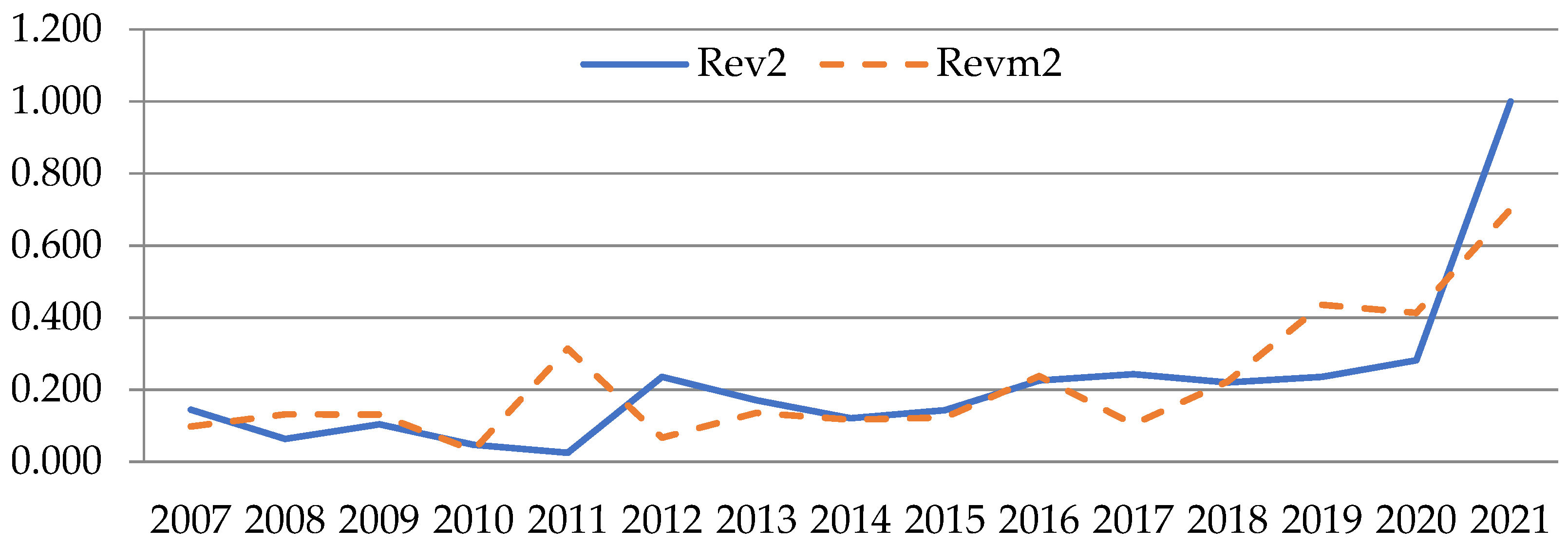
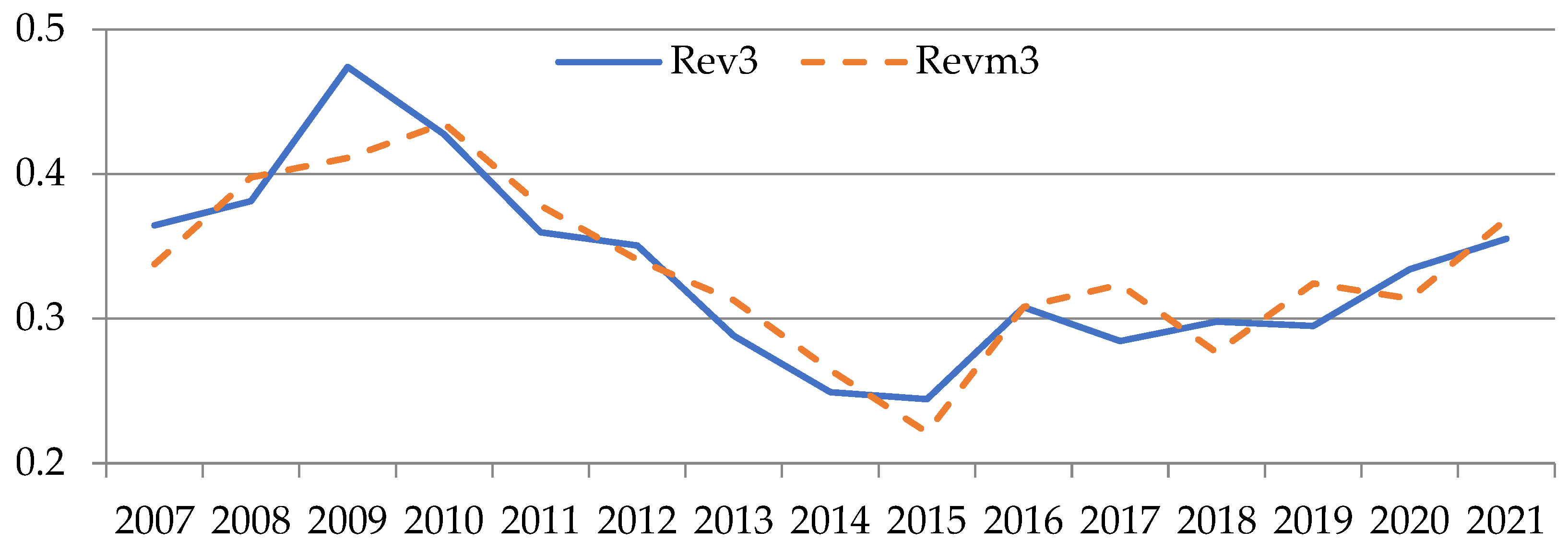
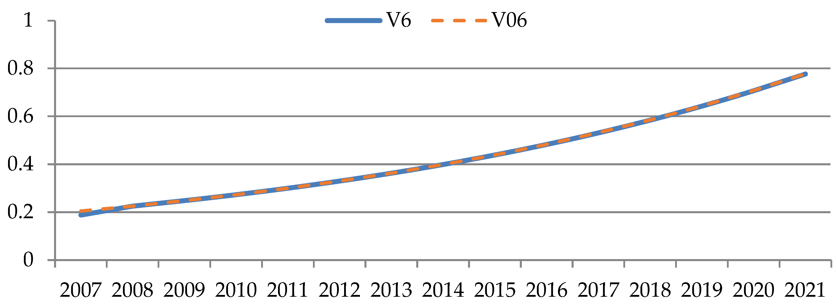
Figure 1, Figure 2, Figure 3, Figure 4, Figure 5 and Figure 6 show comparisons between normalized revenue Revn and the model value of revenue Revm for the 6 sectors under consideration. The values of indicators are plotted along the ordinate axis in conditional values, and along the abscissa axis—the period from 2007 to 2021. The dotted line indicates simulated values, while the solid line indicates actual values.

Simulation results show the correspondence between real and simulated data.

The calculation of the parameters of the indicators change rate ${\mu }_j\left(t\right)$ was carried out on the basis of historical data using the Formula (20)

$${\mu }_j\left(t\right)=\frac{{{\displaystyle \sum }}_{t=2}^T{x}_j\left(t\right)x_j\left(t-1\right)}{{{\displaystyle \sum }}_{t=2}^T{\left(x_j\left(t-1\right)\right)}^2}-1,j=1,\dots ,n$$

(20)

The results of the calculations ${\mu }_j\left(t\right)$ are presented in

Table 5. Parameters of the indicators change rate ${\mu }_j\left(t\right)$ (author’s results).

Sector	μj(t)
No. 1	0.196386	0.616996	0.008233	0.014397	0.00311
No. 2	0.067032	0.820458	0.00479	0.000556	0.006921
No. 3	0.076643	0.735129	0.010589	0.00299	0.020087
No. 4	0.239288	0.58449	0.007383	0.213352	0.001686
No. 5	0.527567	0.350937	0.004393	0.057926	0.005339
No. 6	0.146914	0.690977	0.004453	0.000587	0.018444

.

Let us move on to the problem of managing the company’s revenue. To do this, it is necessary to solve the dynamic programming problem with a quadratic criterion and constraints.

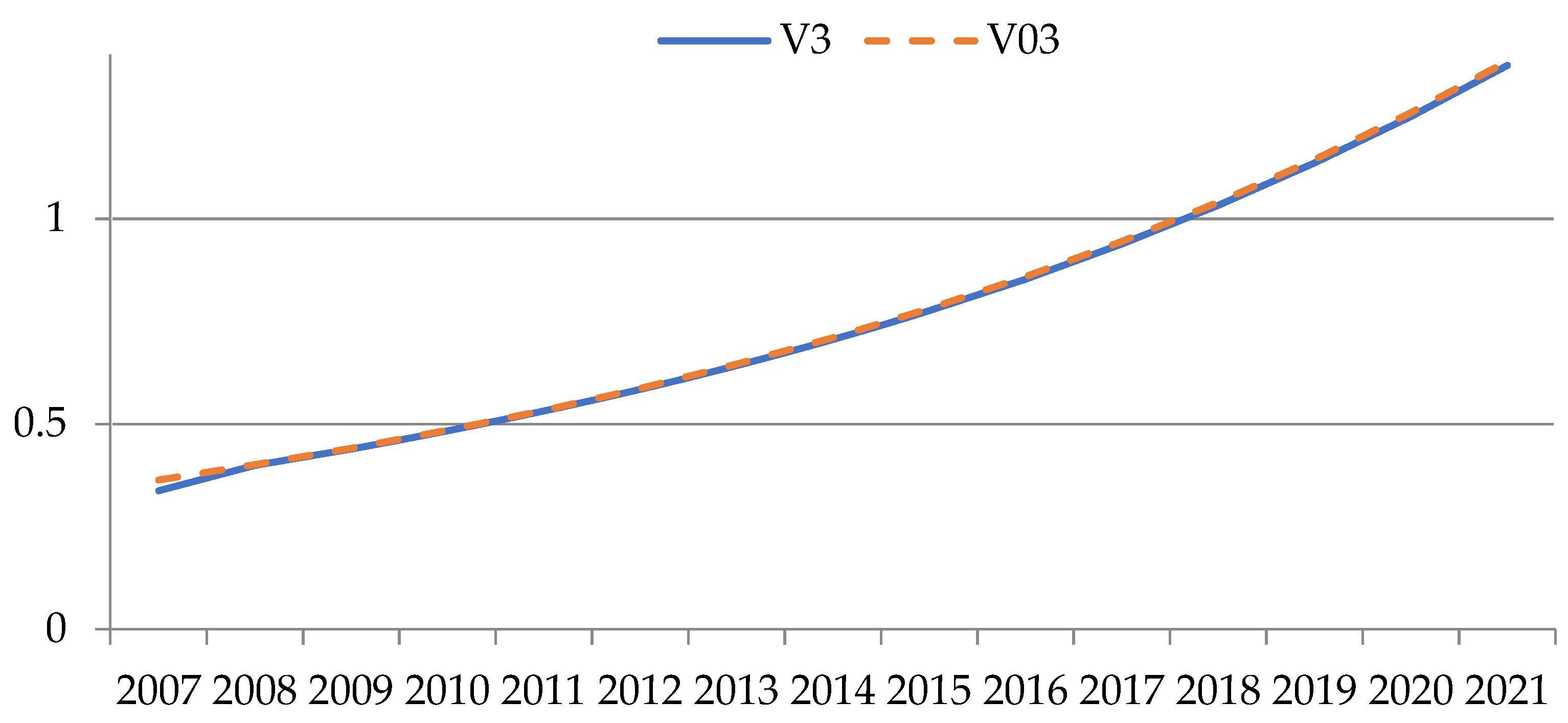
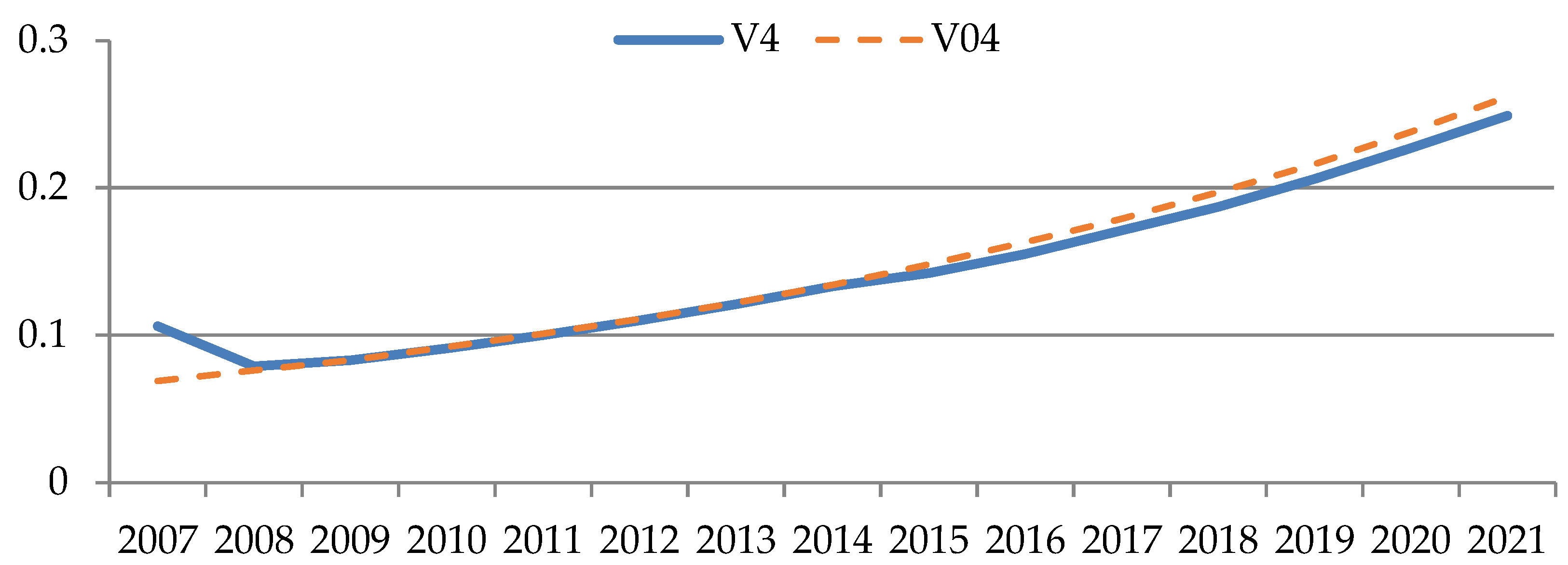
Figure 7, Figure 8, Figure 9, Figure 10, Figure 11 and Figure 12 show the graphs for tracking the planned revenue indicator. The values of the indicator are plotted on the ordinate axis, and the period of years is on the abscissa axis. The line indicates the simulated behavior of the studied indicator ($V^0\left(t\right)$), and the solid line indicates the desired values of the indicator ($V\left(t\right)$).

The efficiency indicator takes a value from 0 to 1. The closer it is to 1, the more efficient the enterprise is, and vice versa, if it is closer to 0, then it is less efficient. To solve the problem, the parameter was set equal to 0.5, $\mathit{eff}$ = 0.5, since it is the average value of the efficiency indicator.

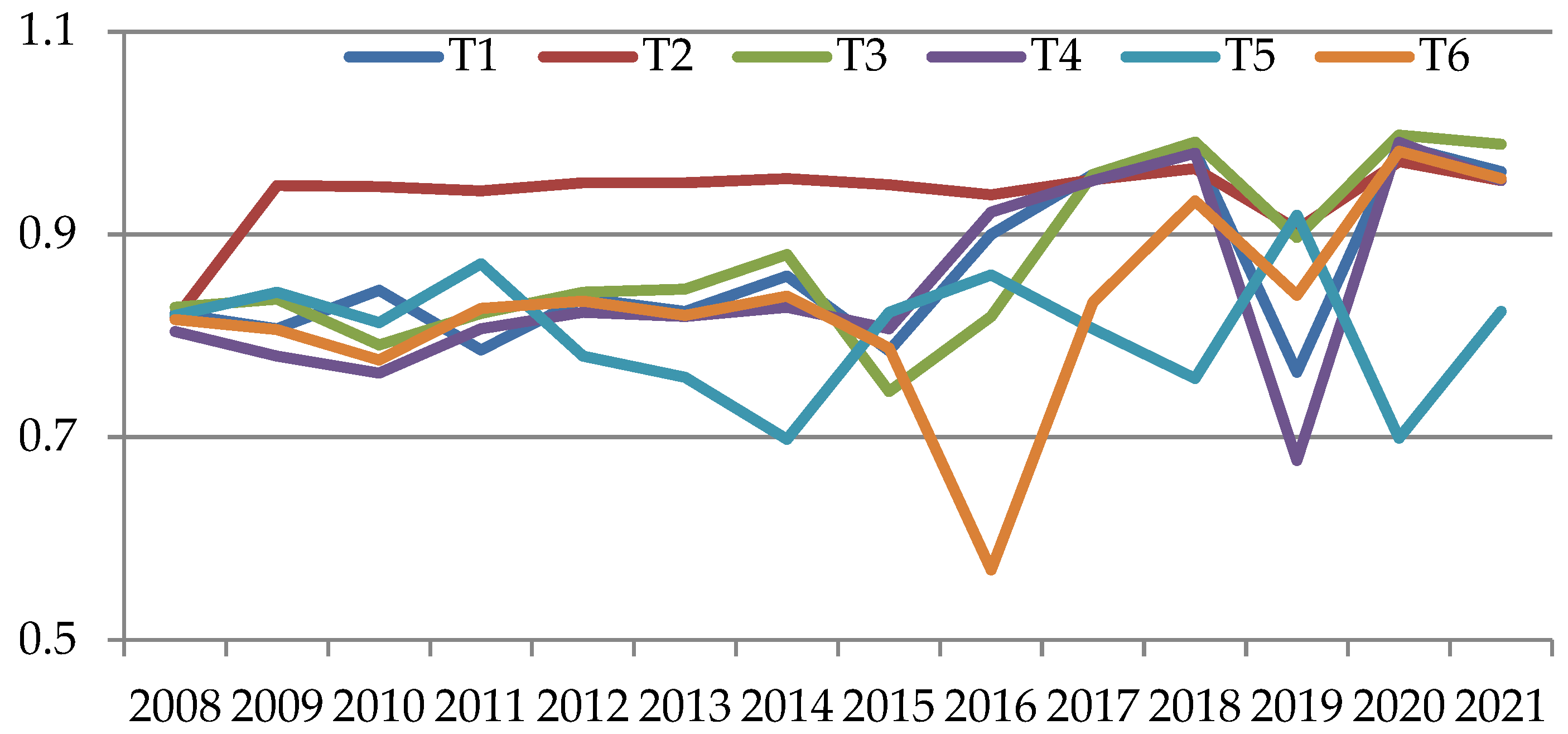
The results of the efficiency assessment of small business sector activities of a single-industry town are presented in

Table 6. Efficiency assessment values (author’s results).

Sector	${\mathit{T}}_{\mathit{j}}^{\mathit{J}\mathit{L}\mathit{M}\mathit{S}}$
	2007	2008	2009	2010	2011	2012	2013	2014	2015	2016	2017	2018	2019	2020	2021
No. 1	0.227	0.822	0.807	0.845	0.786	0.837	0.824	0.859	0.785	0.9	0.959	0.982	0.764	0.988	0.962
No. 2	0.22	0.817	0.948	0.947	0.943	0.951	0.951	0.955	0.949	0.939	0.954	0.965	0.905	0.972	0.953
No. 3	0.22	0.828	0.836	0.791	0.822	0.843	0.846	0.88	0.745	0.819	0.959	0.991	0.897	0.998	0.989
No. 4	0.213	0.804	0.78	0.763	0.807	0.823	0.819	0.828	0.807	0.922	0.953	0.98	0.677	0.991	0.953
No. 5	0.216	0.82	0.843	0.813	0.871	0.78	0.759	0.698	0.823	0.86	0.807	0.758	0.919	0.699	0.824
No. 6	0.223	0.816	0.806	0.776	0.827	0.834	0.82	0.839	0.788	0.569	0.833	0.933	0.84	0.982	0.955

.

Graphs of the behavior of the performance indicator for the two enterprises are shown in Figure 13.

On the basis of the efficiency estimates obtained, it is possible to take preventive measures in order to avoid the bankruptcy of small businesses. To do this, it is necessary to carry out an action plan, which is as follows:

1. Indicators X1 and X2 refer to the assets side of the balance sheet. Regulation by such indicators involves influencing the redistribution of funds between current assets, as well as used non-current assets of the enterprise.

2. Indicators X3, X4, and X5 refer to the liability of the balance sheet. It is possible to manage two such indicators at once as well as to manage all indicators simultaneously. Regulation by such indicators consists of the redistribution of money between capital, reserves, as well as long-term (short-term) obligations of the enterprise. For example, a decrease in the volume of short-term liabilities is possible with the attraction of loans and borrowings on a long-term basis.

6. Conclusions

In the course of the work, an algorithm for solving a dynamic programming problem with a square deviation was developed. The constructed one-factor dynamic model allows organizing the process of managing the company’s revenue.

These graphs show the results of calculations, from which it follows that in order to achieve planned sustainable revenue values, such a constraint as efficiency can be used.

References

1. Telipenko, E.V.; Zakharova, A.A. Bankruptcy risk management of a machine builder. Appl. Mech. Mater. 2014, 682, 17–622. [Google Scholar] [CrossRef]
2. Modeli Bankrotstva (Diagnostika i Otsenka Veroiatnosti Bankrotstva). Available online: http://finance-m.info/bankruptcy_models.html (accessed on 20 September 2022). (In Russian).
3. Altman, E.I. Corporate Financial Distress; Wiley: New York, NY, USA, 1983; 368p. [Google Scholar]
4. Altman, E.I.; Haldeman, R.G.; Narayanan, P. ZETA analysis: A new model to identify bankruptcy risk of corporations. J. Bank. Financ. 1977, 1, 29–54. [Google Scholar] [CrossRef]
5. Altman, E.I. Financial Rations. Discriminate analysis, and the prediction of corporate bankruptcy. J. Financ. 1968, 23, 589–609. [Google Scholar] [CrossRef]
6. Chetyrekhfaktornaia Model’ R. Lisa Otsenki Riska Bankrotstva. Available online: http://www.beintrend.ru/2011-12-05-17-20-28 (accessed on 20 September 2022). (In Russian).
7. Mitsel, A.A.; Soboleva, M.A. Analysis of financial sustainability of Russian cellular communication enterprises. J. Financ. Anal. Sci. Exp. 2015, 8, 24–31. [Google Scholar]
8. Fulmer, J.G.; Moon, J.; Gavin, T.A.; Erwin, M.J. A bankruptcy classification model for small firms. J. Commer. Bank Lend. 1984, 66, 25–37. [Google Scholar]
9. Prognoznaia Model’ Platezhesposobnosti Springeitava. Available online: http://afdanalyse.ru/publ/finansovyj_analiz/1/prognoznaja_model_platezhesposobnosti_springejta/13-1-0-39 (accessed on 21 September 2022). (In Russian).
10. Model’ Prognozirovaniia Bankrotstva Predpriiatiia Springeita. Available online: http://beintrend.ru/springate (accessed on 20 September 2022). (In Russian).
11. Taffler, R.J.; Tisshaw, H. Going, going, gone—Four factors which predict. Accountancy 1977, 88, 50–54. [Google Scholar]
12. Model’ Bankrotstva Predpriiatii Saifullina-Kadykova. Available online: http://www.beintrend.ru/2011-06-20-17-05-06 (accessed on 21 September 2022). (In Russian).
13. Sheremet, A.D.; Saifulin, R.S. Metodika Finansovogo Analiza Predpriiatiia [Methodology of Financial Analysis of the Enterprise]; Business: Moscow, Russia, 1998; 320p. [Google Scholar]
14. Davydova, G.V.; Belikov, A.I. Metodika kolichestvennoi otsenki riska bankrotstva predpriiatii [Methodology of quantitative assessment of the risk of bankruptcy of enterprises]. Risk Manag. 1999, 3, 13–20. [Google Scholar]
15. Zaitseva, O.P. Antikrizisnyi Menedzhment v Rossiiskoi Firme [Anti -Crisis Management in the Russian Company]. Sib. Financ. Sch. 1998, 11–12, 66–73. [Google Scholar]
16. Makareva, V.I.; Andreeva, L.V. Analiz Finansovo-Khoziaistvennoi Deiatel’nosti Predpriiatiia [Analysis of the Financial and Economic Activities of the Enterprise]; Finance and Statistics: Moscow, Russia, 2004; 264p. [Google Scholar]
17. Telipenko, E.V.; Zakharova, A.A. Problemy prognozirovaniia riska bankrotstva predpriiatii mashinostroitel’nogo kompleksa [Problems of predicting the risk of bankruptcy of enterprises of the engineering complex]. In Innovative Technologies and Economics in Mechanical Engineering: A Collection of Works of the VI International Scientific and Practical Conference; Tomsk Polytechnic University: Tomsk, Russia, 2015; pp. 262–266. [Google Scholar]
18. Mitsel, A.A.; Kabalin, A.A. Modeli riska i prognozirovaniia bankrotstva predpriiatiia [Models of risk and prediction of bankruptcy of the enterprise]. Risk Manag. 2013, 1, 44–52. [Google Scholar]
19. Vazhdaev, A.N.; Mitsel, A.A. One-Factor Dynamic Model to Manage Small Businesses in a Single-Industry City. J. Econ. Anal. Theory Pract. 2018, 17, 950–966. [Google Scholar] [CrossRef]
20. Coelli, T.; Prasada Rao, D.S.; Battese, G.E. An Introduction to Efficiency and Productivity Analysis; Springer: New York, NY, USA, 1998; 276p. [Google Scholar]
21. Battese, G.E.; Coelli, T.J. Prediction of firm-level technical efficiencies with a generalized frontier production function and panel data. J. Econom. 1988, 38, 387–399. [Google Scholar] [CrossRef]
22. Jondrow, J.; Lovell, C.A.K.; Materov, I.S.; Schmidt, P. On the estimation of technical inefficiency in stochastic frontier production function model. J. Econom. 1982, 19, 233–239. [Google Scholar] [CrossRef] [Green Version]
23. Malakhov, D.I.; Pilnik, N.P. Methods of estimating of the efficiency in stochastic frontier models. Ekon. Zhurnal VSE 2013, 4, 660–686. [Google Scholar]
24. Wheelock, D.C.; Wilson, P.W. Explaining bank failures: Deposit insurance, regulation, and efficiency. Rev. Econ. Stat. 1995, 4, 689–700. [Google Scholar] [CrossRef] [Green Version]
25. Dimara, E.; Skuras, D.; Tsekouras, K.; Tzelepis, D. Productive efficiency and firm exit in the food sector. Food Policy 2008, 33, 185–196. [Google Scholar] [CrossRef]
26. Barr, R.S.; Siems, T.F. Bank Failure Prediction Using Dea to Measure Management Quality. In Interfaces in Computer Science and Operations Research; Barr, R.S., Helgason, R.V., Kennington, J.L., Eds.; Operations Research/Computer Science In-terfaces Series; Springer: Boston, MA, USA, 1997; Volume 7, pp. 341–365. [Google Scholar] [CrossRef]
27. González, J.S.; Restrepo-Tobón, D.; Hassan, A.R. Inefficiency and bank failure: A joint Bayesian estimation method of stochastic frontier and hazards models. Econ. Model. 2021, 95, 344–360. [Google Scholar] [CrossRef]
28. Sun, K.; Salim, R. A semiparametric stochastic input distance frontier model with application to the Indonesian banking in-dustry. J. Product. Anal. 2020, 54, 139–156. [Google Scholar] [CrossRef]
29. Hwang, R.-C.; Siao, J.-S.; Huimin, C.; Chu, C.K. Assessing bankruptcy prediction models via information content of technical inefficiency. J. Product. Anal. 2011, 36, 263–273. [Google Scholar] [CrossRef] [Green Version]
30. Merton, R.C. On the pricing of corporate debt: The risk structure of interest rates. J. Financ. 1974, 29, 449–470. [Google Scholar]
31. Shumway, T. Forecasting bankruptcy more accurately: A simple hazard model. J. Bus. 2001, 74, 101–124. [Google Scholar] [CrossRef] [Green Version]
32. Mogilat, A.; Ipatova, I. Technical efficiency as a factor of Russian industrial companies’ risks of financial distress. J. Appl. Econoimetr. 2016, 42, 5–29. [Google Scholar]
33. Van Nguyen, Q.; Pascoe, S.; Coglan, L.; Nghiem, S. The sensitivity of efficiency scores to input and other choices in stochastic frontier analysis: An empirical investigation. J. Product. Anal. 2021, 55, 31–40. [Google Scholar] [CrossRef]
34. Despic, D.R.; Bojovic, N.J.; Kilibarda, M.J.; Kapetanovic, M.V. Assessment of efficiency of military transport units using the DEA and SFA methods. Vojnoteh. Glas. 2019, 67, 68–92. [Google Scholar] [CrossRef]
35. André, C.; Pareliussen, J.; Hwang, H. Swedish School Results, Student Background, Competition and Efficiency. Educ. Stud. Mosc. 2020, 3, 8–36. [Google Scholar]
36. Ponkina, E.V.; Kurochkin, D.V. Technical Efficiency in Crop Production: Measurement Based on Econometric Methods of Data Envelopment Analysis and Stochastic Frontier Analysis. Izv. Altai State Univ. 2014, 1, 170–178. [Google Scholar] [CrossRef]
37. Aivazian, S.A.; Afanasiev, M.Y.; Rudenko, V.A. Efficiency estimation of the russian regions based on the productive potential model including the characteristics of readiness to innovate. Econ. Math. Methods 2014, 50, 34–70. [Google Scholar]
38. Vasanthi, R.; Sivasankari, B.; Gitanjali, J. A stochastic frontier and corrected ordinary least square models of determining technical efficiency of canal irrigated paddy farms in Tamil Nadu. J. Appl. Nat. Sci. 2017, 2, 658–662. [Google Scholar] [CrossRef] [Green Version]
39. Riabchenko, A.V. Otsenka effektivnosti strakhovykh kompanii. SFA-podkhod [Assessment of the effectiveness of insurance companies. SFA approach]. Bull. Khabarovsk State Acad. Econ. Law 2012, 1, 97–106. [Google Scholar]
40. Papadopoulos, A.; Parmeter, C.F. Quantile Methods for Stochastic Frontier Analysis. Found. Trends Econom. 2022, 12, 1–120. [Google Scholar] [CrossRef]
41. Vazhdaev, A.N.; Mitsel, A.A. Technology of preliminary data preparation by city indicators and microindicators of small business for investigation of their dependencies (on the example of the single-industry town of Yurga). In Proceedings of the International Scientific and Practical Conference “New Technologies in Science, Education, Production”, Ryazan, Russia, 10–13 November 2017; pp. 34–45. [Google Scholar]
42. Vazhdaev, A.N. Technology of downloading data of accounting reporting of small business enterprises from the service of contract inspection (on the example of the single-industry town of Yurga). Fundam. Res. 2017, 5, 31–35. [Google Scholar]
Figure 1. Comparison between real revenue and model value calculated by Formula (1) for industry No. 1 (author’s results).
Mathematics 11 00211 g001
Figure 2. Comparison between real revenue and model value calculated by Formula (1) for industry No. 2 (author’s results).
Mathematics 11 00211 g002
Figure 3. Comparison between real revenue and model value calculated by Formula (1) for industry No. 3 (author’s results).
Mathematics 11 00211 g003
Figure 4. Comparison between real revenue and model value calculated by Formula (1) for industry No. 4 (author’s results).
Mathematics 11 00211 g004
Figure 5. Comparison between real revenue and model value calculated by Formula (1) for industry No. 5, (author’s results).
Mathematics 11 00211 g005
Figure 6. Comparison between real revenue and model value calculated by Formula (1) for industry No. 6, (author’s results).
Mathematics 11 00211 g006
Figure 7. Graphs for tracking the target revenue indicator for industry No. 1 (author’s results).
Mathematics 11 00211 g007
Figure 8. Graphs for tracking the target revenue indicator for industry No. 2 (author’s results).
Mathematics 11 00211 g008
Figure 9. Graphs for tracking the target revenue indicator for industry No. 3 (author’s results).
Mathematics 11 00211 g009
Figure 10. Graphs for tracking the target revenue indicator for industry No. 4 (author’s results).
Mathematics 11 00211 g010
Figure 11. Graphs for tracking the target revenue indicator for industry No. 5 (author’s results).
Mathematics 11 00211 g011
Figure 12. Graphs for tracking the target revenue indicator for industry No. 6 (author’s results).
Mathematics 11 00211 g012
Figure 13. Graph of the behavior of performance indicators for sectors.
Mathematics 11 00211 g013