Abstract
Intelligent robotics has drawn a great deal of attention due to its high precision, stability, and reliability, which are the basic key factors for industrial automation. This paper proposes an iterative learning control (ILC) technique with predefined-time convergence as a solution to an applied engineering problem, namely, that local time cannot be preset when a second-order nonlinear system undertakes control of the accurate tracking of local time under any initial iterative value. A time-varying sliding surface with an initial value of zero was designed, and it was theoretically proven that the trajectory tracking error in the sliding surface could converge to zero within a predefined time. The iterative control problem of trajectory tracking was thus changed to an iterative control problem of time-varying sliding-mode surface tracing with a starting value of zero. A PD-type closed-loop ILC with a time-varying sliding mode surface was designed such that the trajectory tracking error converged and stabilized on the sliding mode surface after a finite number of learning iterations. The control goal for the system’s output was the ability to track the desired trajectory accurately within a predefined time interval, and it was achieved by combining this with the predefined time convergence characteristics of the time-varying sliding mode surface. Numerical simulation of trajectory tracking control of a repetitive motion manipulator was used to verify the effectiveness of the proposed controller and its robustness in the face of external disturbances.
Keywords:
iterative learning control; sliding mode control; predefined-time convergence; time-varying sliding mode surface; robotic arm MSC:
393D05; 37N35
1. Introduction
In engineering applications such as industrial recurrent production, hard disk drive control, and construction robot wall building, the output of the repetitive motion control system is required to move a mechanical arm strictly according to the desired trajectory within a finite time interval . When the initial value of trajectory tracking error is zero, iterative learning control (ILC) is implemented. In short, ILC can ensure that the system output fully tracks the desired trajectory [1,2], but in practical engineering applications it is challenging to strictly locate the initial state of the controlled system at the initial position of the desired trajectory. The arbitrary initial value of iterative learning control can only ensure that the system output accurately tracks the desired trajectory in local time , but the existing ILC control strategy cannot be preset or estimated in the bound of time . This restricts the application of ILC in practical engineering. Therefore, there is a strong need to design an iterative learning control algorithm with a predefined time of .
Traditional ILC control theory is predicated on the assumption that the controlled system’s iterative starting value deviation is zero. When the controlled system is satisfied with the iterative initial value constraint conditions, the output of the controlled system can be in a given time interval, in strict accordance with the desired trajectory [3,4,5] (which is perfect tracking), but in practical engineering applications, it is difficult to meet every time constraint with a zero initial iteration value deviation [6]. Thus, the engineering application of ILC theory is limited. Scholars have confirmed, through theoretical analysis and experimental verification, that when the deviation between the initial value of the controlled system and the desired trajectory is a fixed value, or when the initial value of the system and the desired trajectory satisfy a certain law, this value of the system can converge to the initial value of the desired trajectory, for which the ILC algorithm can also ensure that the output of the controlled system follows the desired trajectory [7,8] (for instance, the tracking accuracy in fractional order control [9,10] and optimal learning control [11]). This result relaxes the strict requirement that the iterative initial value variation of the conventional ILC must be zero [12,13], but it is still compatible with real-world engineering applications. When a difference arises, only iterations of the ILC control algorithm that satisfy the initial value criteria will be able to fulfil the needs of the practical engineering application.
Scholars have proposed control strategies such as model predictive control, the initial value correction method, the boundary layer method, and the attractor method [14,15,16], but the initial value correction method involves determining the delay factor in advance [17,18].The boundary layer in the boundary layer method is asymptotically convergent, which means that the trajectory tracking error in the boundary layer can only converge to zero when time tends to infinity, resulting in low trajectory tracking accuracy [19]. The attractor design in the attractor method has certain limitations, and some attractor control strategies involve redesigning the desired trajectory [20].When the initial value of the tracking error between the system output and the desired trajectory is , after a finite number of iterations the system output has the full ability to follow the desired trajectory within the finite time interval, . However, when the initial value of the tracking error between the system output and the desired trajectory is , it means that particular system is able only to track the desired signal within the local time interval , which is . Although the existing control strategies to suppress the initial value of any iteration can solve the iterative learning convergence problem under the initial value of any iteration, they cannot estimate or even set the time, , to achieve local convergence in advance. In some practical engineering applications, it is required that the system output accurately tracks the desired trajectory before the given time, . For example, when a construction robot performs construction processes such as concrete troweling or wall laying, the mechanical arm must reach the desired trajectory before the given time, , and repeat the movement strictly according to the desired trajectory to ensure the smoothness of concrete troweling or the uniformity of wall tiles. Failure to achieve this can lead to major economic losses for the construction industry, as well as raise the risk of building collapse. Despite the importance of determining and presetting the local convergence time in many engineering applications, very little work has been done on the iterative learning control theory in regard to predefined-time convergence. At the same time, while many current iterative learning control strategies under arbitrary iterative initial values have been projected mainly for first-order systems, there are relatively few publications on iterative learning control strategies for second-order nonlinear systems under arbitrary iterative initial values.
This paper will focus on second-order nonlinear systems with repetitive motion, and propose a PD-type closed-loop iterative learning control strategy based on the predefined-time convergence sliding mode surface, aiming to show that the controlled system under any initial value can not only follow a local trajectory for accurate tracking, but also predetermine the local convergence time, , in advance. The main innovations and contribution of this study can be summarized as follows:
- Provides Lyapunov stability criterion for the stability of nonlinear systems within a predefined time and describes the theoretical proof under the given conditions.
- Presents a design for a time-varying sliding mode surface with predefined time convergence characteristics in which the convergence time of the trajectory tracking error located in the sliding mode surface can be preset, bringing the advantage that the convergence time is not affected by the controlling constraints or the initial value of the iteration.
- Converts the trajectory tracking control problem, where the initial value of the trajectory tracking error is not zero, into a sliding mode surface tracking control problem in which the initial value of the sliding mode surface being zero. Establishes a bridge between the iterative learning control theory with an arbitrary iterative initial value and the same iterative initial value.
- The iterative learning control strategy not only solves the problem of arbitrary iterative initial value suppression and simplifies the theoretical proof of the convergence of iterative learning, it also achieves the engineering application of the system output, accurately tracking the desired trajectory within a preset local time.
The remainder of this paper is as follows. Section 2 presents the control problem formulation and also describes several lemmas for iterative learning convergence proof. Section 3 proposes an arbitrary initial value suppression strategy based on the predefined time convergence sliding mode control principle, mentioning its principles. The Lyapunov stability criterion for predefined time convergence of nonlinear systems is given, and a design for a sliding mode surface with the character of predefined time convergence and initial value of zero is presented. The main results of iterative convergence are discussed in Section 4, which also demonstrates the predefined time convergence condition for a PD-type ILC. In Section 5, the effectiveness of the proposed nonlinear control strategy is illustrated by simulations for a robotic system, the results of which are briefly explained. Finally, Section 6 presents the conclusions.
2. Control Problem Descriptions
Consider the following second-order nonlinear system with repetitive motion characteristics:
where indicates the state variable, is the output variable, is the control input variable, represents the number of iterations, and , is the bounded function matrix of appropriate dimension. The function satisfies the Lipschitz condition with respect to the state variable, , in the time interval . That is means there is a constant,, and function satisfies
The control objective: Let the desired trajectory of the second-order nonlinear system (1) be in an application environment where the iterative initial value, , of the second-order nonlinear system (1) cannot be strictly located at the initial value, , of the desired trajectory. Design an iterative learning controller, , to make the output of system (1) precisely track the desired trajectory, , over a predefined-time interval, .
The tracking error between the system output, , and the target trajectory, , may be determined as follows:
Below are some lemmas for iterative learning convergence proof:
Lemma 1 .
Let be a continuous function defined on the interval , and . If [21]
then .
Lemma 2 .
Suppose that the mentioned function, , for the time interval mollifies the following conditions [21]:
- (1)
- (2)
In the above formula, if
and
are non-negative constants, then we can draw the following two conclusions:
- (a)
- For , there exists a unique , such that
- (b)
- According to the definition of the function defined as , where is the only solution defined by (a), there exists an such that
Lemma 3 .
Let the constant series converge to zero, and the function satisfy [21]
In the previous expression,
is a constant. If we assume that
, which can be
, is a dimensional matrix of continuous functions, and
, then:
From the above equations, it follows that when the spectral radius of
< 1, then:
3. Arbitrary Initial Value Suppression Strategy Based on Predefined-Time Convergence Sliding Mode Surface
3.1. Arbitrary Initial Value Suppression Strategy and Its Principle
According to the sliding mode control principle [22], a system state whose initial value is located at any position in the state space can reach and stabilize in the sliding mode surface under the sliding mode controller and within the sliding mode surface (equivalent to ) sliding to the equilibrium point, . The sliding mode control (SMC) law is illustrated in Figure 1.
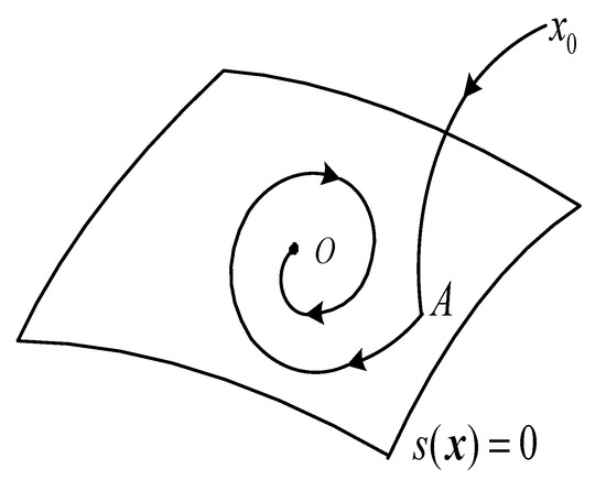
Figure 1.
Schematic diagram of the principle, sliding mode control principle.
This study offers an arbitrary iterative initial value suppression control technique based on a predefined-time convergence sliding mode surface to tackle the arbitrary starting value issue in iterative learning control, using a control goal system (1) and the SMC principle.
When the starting state of the k-th iterative learning is at any point in space, it is the same as the initial value of trajectory or route tracking errors, . By applying the SMC concept, it is possible to build a sliding mode surface,,with predefined-time convergence characteristics and an iterative learning controller, , allowing the controller, ,to drive errors,, that arrive at any starting position and stabilize in the sliding mode surface (equivalent to ). When the tracking error is stabilized in the sliding mode surface according to the predefined-time convergence characteristics of the SMC surface, and when the tracking error, , returns to zero within the predetermined period, ; that is, when , the goals of suppressing the issue of random starting values and achieving precise tracking of the intended trajectory are both realized.
To achieve the trajectory tracking error satisfying within the predefined-time interval , several core problems present themselves. The first is ensuring that the tracking error, , converges and stabilizes within the sliding mode surface after finite iterative learning, that is, . The second is that in the sliding mode surface , trajectory tracking error converges to the equilibrium point in a predefined-time, , that is, . Based on the above two core problems, this paper designs a controller that suppresses the arbitrary iterative initial value problem in two steps. The first step is to design the sliding mode surface with the characteristic of converging to the equilibrium point within the predefined-time, , to ensure that the tracking error in sliding mode surface converges to the equilibrium point within the predefined-time, . The second step is to design an iterative learning controller to ensure the convergence of iterative learning, so that the tracking error reaches and stabilizes in the sliding surface .
3.2. Predefined-Time Convergence Lyapunov Stability Criterion and Sliding Mode Surface Design
Predefined-time convergence is the key to suppressing the arbitrary initial value of iteration and ensuring that the trajectory tracking error can achieve accurate tracking before the predefined-time, . The definition of predefined-time stability is given below.
Definition 1.
For a second-order nonlinear system (1), if there is a preset constant, , such that for any the condition is satisfied:
Then the second-order nonlinear system (1) is globally predefined-time stable.
A Lyapunov stability criterion of the predefined-time convergence is presented below and proven theoretically in order to facilitate the assessment of the nonlinear system’s global predefined-time convergence.
Theorem 1.
In a nonlinear system (1), for any given predefined-time, , if there exsits a positively definite and radially unbounded Lyapunov function, , which satisfies
where the parameters satisfy , then
- (1)
- if , then the system is global predefined-time stable and converges to the equilibrium time: and
- (2)
- f , then , meaning that the system state is always at the equilibrium point.
Proof .
According to , adding the nonnegative constant to the right hand means that
changes it format, giving:
After transforming (11), we obtain
After compiling differentiation (12), in order to make the integration process simpler, we have
Assume that at time and integrate both sides of Equation (13) simultaneously on . Since , , then and, according to , we have:
When , , it means that is always true, indicating that the system state has always been at the equilibrium point. □
The predefined-time convergence stability criterion of the nonlinear system is mainly used to determine whether the trajectory tracking error located in the sliding mode surface can converge to the origin within a predefined time. We can derive a predefined-time sliding mode surface. The main goal of the proposed surface is to converge at that particular predefined time. This kind of time-varying sliding surface with predefined time characteristics can be described as follows:
where the parameters satisfy , is the predefined-time, and is a smaller constant that satisfies . Subsequently, a trajectory tracking error, , in the sliding mode surface may go to zero within a predefined-time , which is given in the form of a theorem, and can be proved theoretically.
Theorem 2.
For any predefined-time , when the sliding mode surface (15) satisfies , it shows that the error will converge to zero within the predefined-time, , and the convergence time is:
where .
Proof.
Note variable as:
When has , establish the Lyapunov function as , and derive it to get
where . Due to the fact that satisfies , and contains the exponent part , when takes a larger value, can quickly tend to zero, so the influence of on is very small and (18) can actually be equivalent to:
According to Theorem 1, when the sliding mode surface (15) fulfils the condition , which implies an error, , it may converge to zero within the predefined-time, with a convergence time of
From the above analysis, it can be seen that the predefined-time convergence sliding mode iterative learning control strategy proposed in this paper can be described as designing an iterative learning controller for a sliding mode surface, , so that the sliding mode surface converges to 0 after iterative learning. This means that the trajectory tracking error, , will converge to 0 within the predefined-time, , achieving the control purpose of accurately tracking the desired trajectory within the preset interval . □
This control strategy transforms the trajectory tracking control problem with an initial trajectory tracking error value that is not zero into a sliding mode surface tracking control problem with the initial value of the sliding surface at zero. It also establishes a bridge connecting the iterative learning control theory of arbitrary iterative initial value and the same iterative initial value. The theoretical connecting bridge not only solves the arbitrary initial value problem of iteration but also simplifies the theoretical proof of the convergence of iterative learning and can take advantage of the existing theoretical achievements of iterative learning control.
For convenience, in the theoretical proof of the convergence of iterative learning, we will take as .
4. Convergence Analysis of PD-Type ILC
To ensure that the output of the nonlinear system accurately tracks the desired trajectory within the predefined-time interval, , the sliding mode surface must converge to zero. Therefore, let the desired trajectory of the sliding mode surface be , and , then denote the tracking error .
The PD-type closed-loop iterative learning controller for sliding mode surfaces is designed as:
where is proportional gain matrix, is differential gain matrix, and and are positive-definite matrixes.
Theorem 3.
In relation to the second-order nonlinear system defined in (1), if the PD-type iterative learning controller is the controller which is described in (19), and the spectral radius satisfies
then, the sliding mode surface will converge to zero under the condition of , ie .
Proof.
Introduce variable as:
Then
According to Formula (1), we have
where . Because is a function of , and within the time interval , it satisfies the Lipschitz condition regarding and . Therefore, the function also satisfies the Lipschitz condition with variable . That is, there is a constant , with
The unique solution of this differential equation is obtained according to add .
Then:
Then
is deformed to obtain
Note , and is defined as
Then:
According to Formula (25), it can be deduced that:
By taking the norm on both sides of (31) we obtain
where: , , ,
According to Lemma 1, we have:
where . By taking the norm on both sides of Equation (28), we obtain:
where .
Note , has
Similarly, it can be deduced that:
where the constant . According to Lemma 2, the particular function designed as , such that
where satisfies
is a constant in the Formula (38).
Defining the function is ; according to Lemma 3, we know that such that , and
As mentioned in Lemma 3, if the condition of a spectral radius of that is , then is uniformly established for , such that the sliding mode surface, , converges to zero uniformly under the control of PD-type closed-loop iterative learning law.□
According tso Theorem 2, when , which signifies that tracking error, , definitely converges to the equilibrium point within a predefined-time, , then , such that the trajectory tracking error of the nonlinear system under arbitrary initial value of iteration is convergent in the predefined-time that is our control target.
5. Simulation Experiment
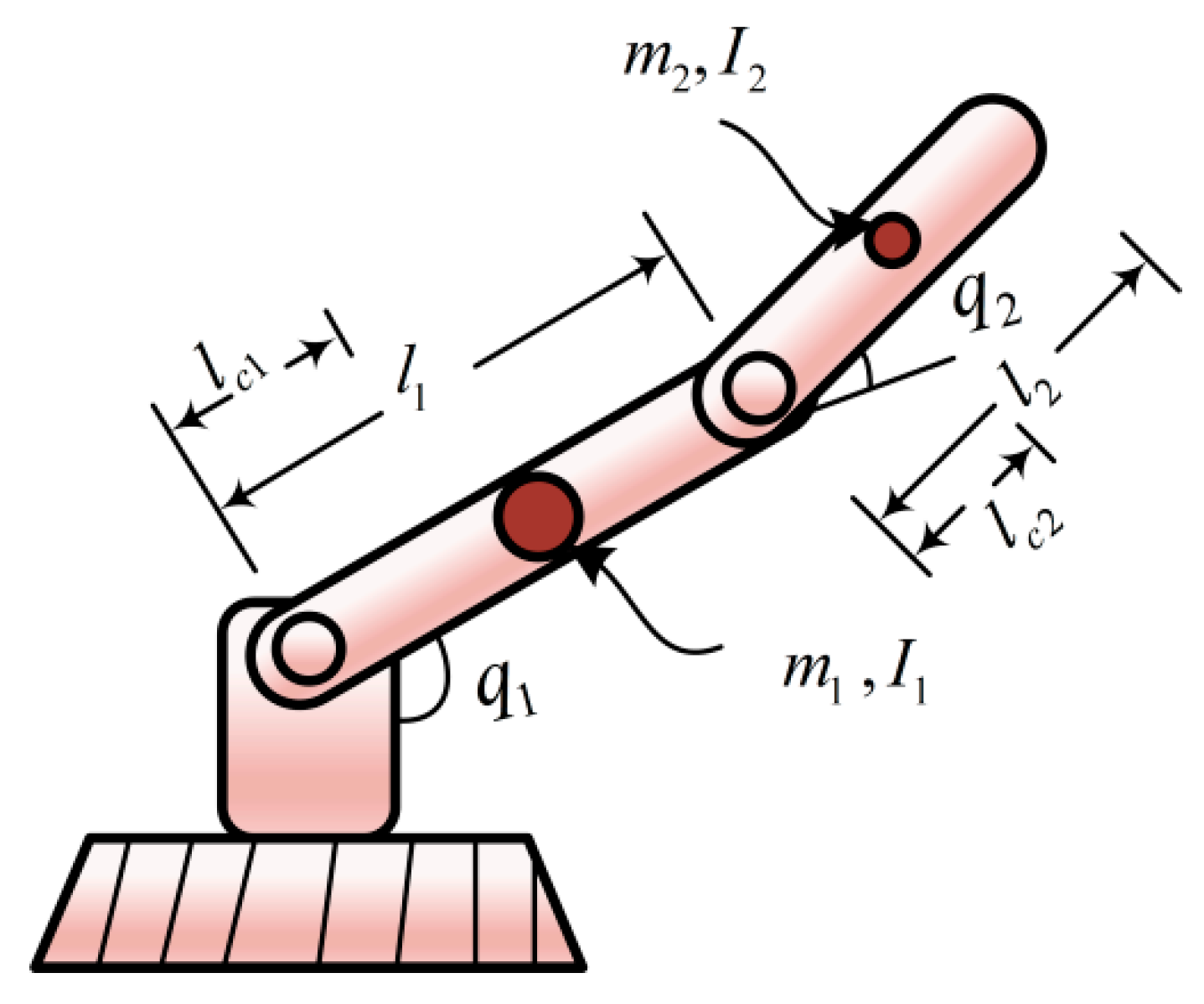
The simulation target of this article is a two degree of freedom (2-DOF) manipulator undergoing repeated motion within the control of a trajectory tracking controller, as shown below. The manipulator’s dynamic model is described as follows (see below Figure 2):
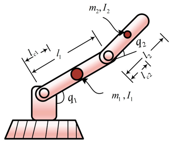
Figure 2.
Two degree of freedom manipulator.
In the above-mentioned Equation (39), denote the joint position, velocity, and acceleration of the manipulator respectively. denotes the inertial matrix, signifies the centripetal force matrix, shows the gravity vector, and denotes the control input. The expressions of the elements in the matrices , , and are: , , , , , , , , , ,
The relevant parameters of the manipulator are listed in Table 1.

Table 1.
Parameters of robotic manipulator.
The simulation time was set to 20 s, the number of iterations to 10, and the predefined convergence time to . With the Matlab command = (rand (4, 1)−0.5).*10, we produced a random initial point for each iteration, which we then used to determine the initial value of the position and velocity of iterative learning.
The controller parameters for the simulation investigation are given in Table 2.

Table 2.
Controller parameters.
5.1. Case 1: Control Performance (Without Disturbances)
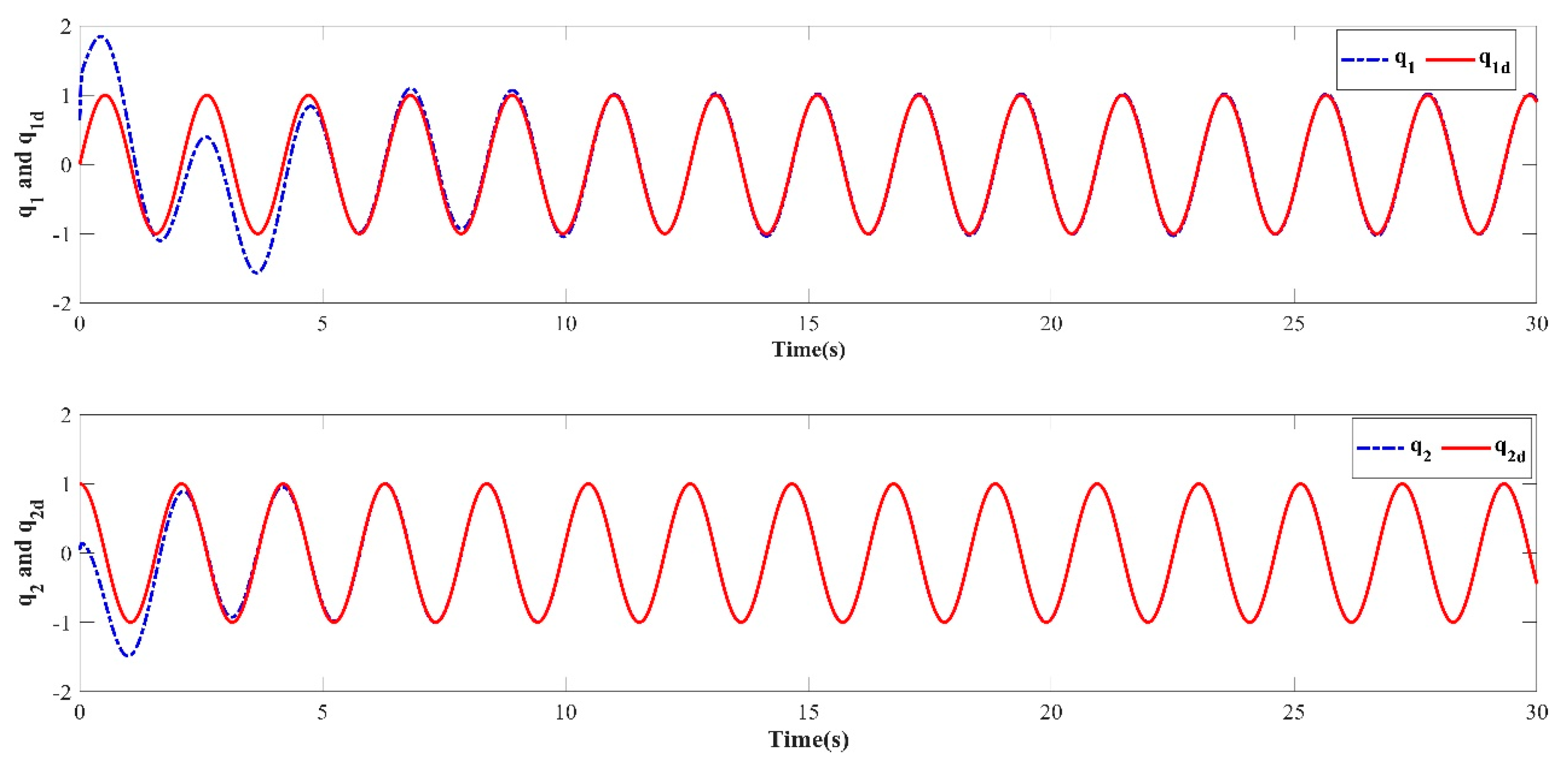
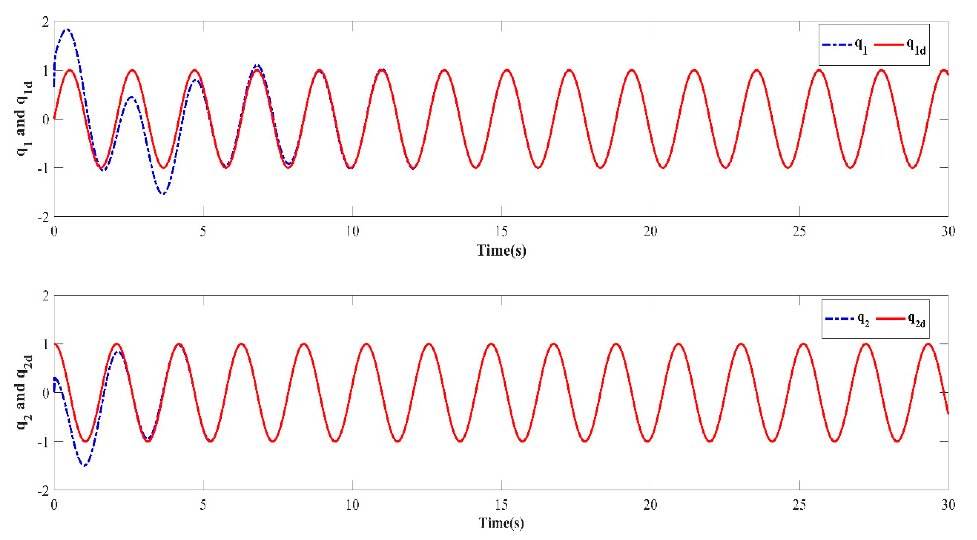
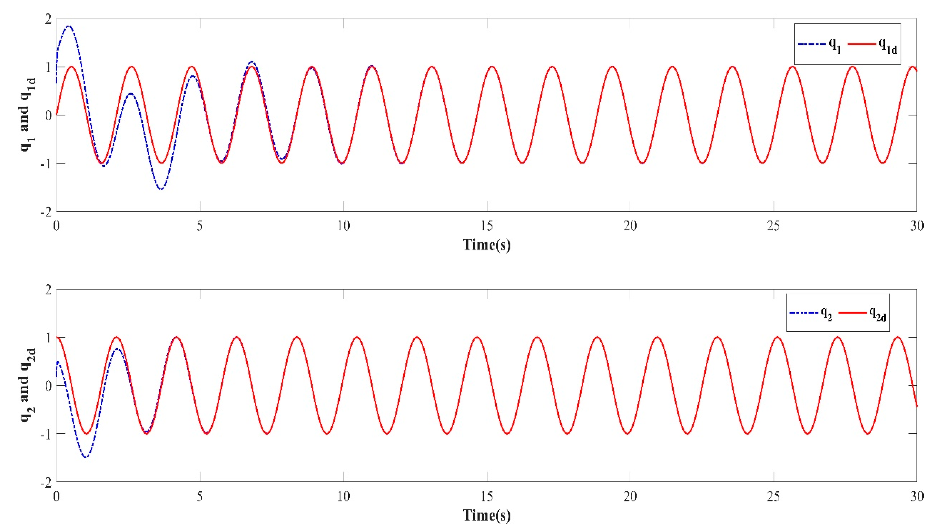
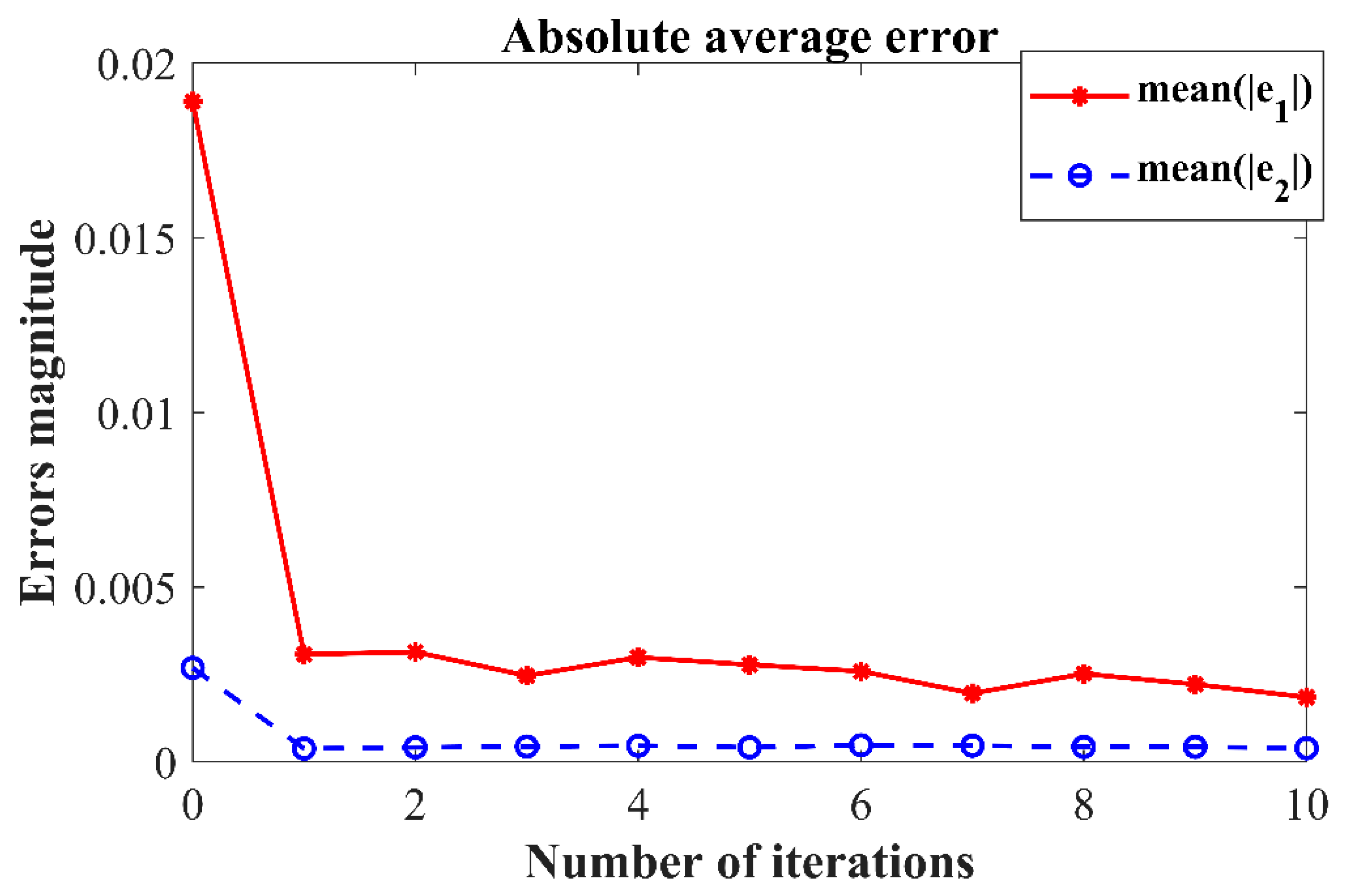
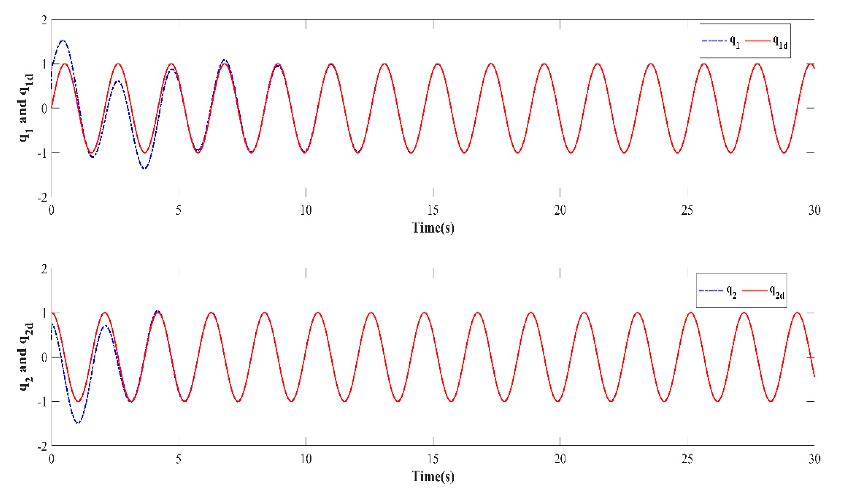
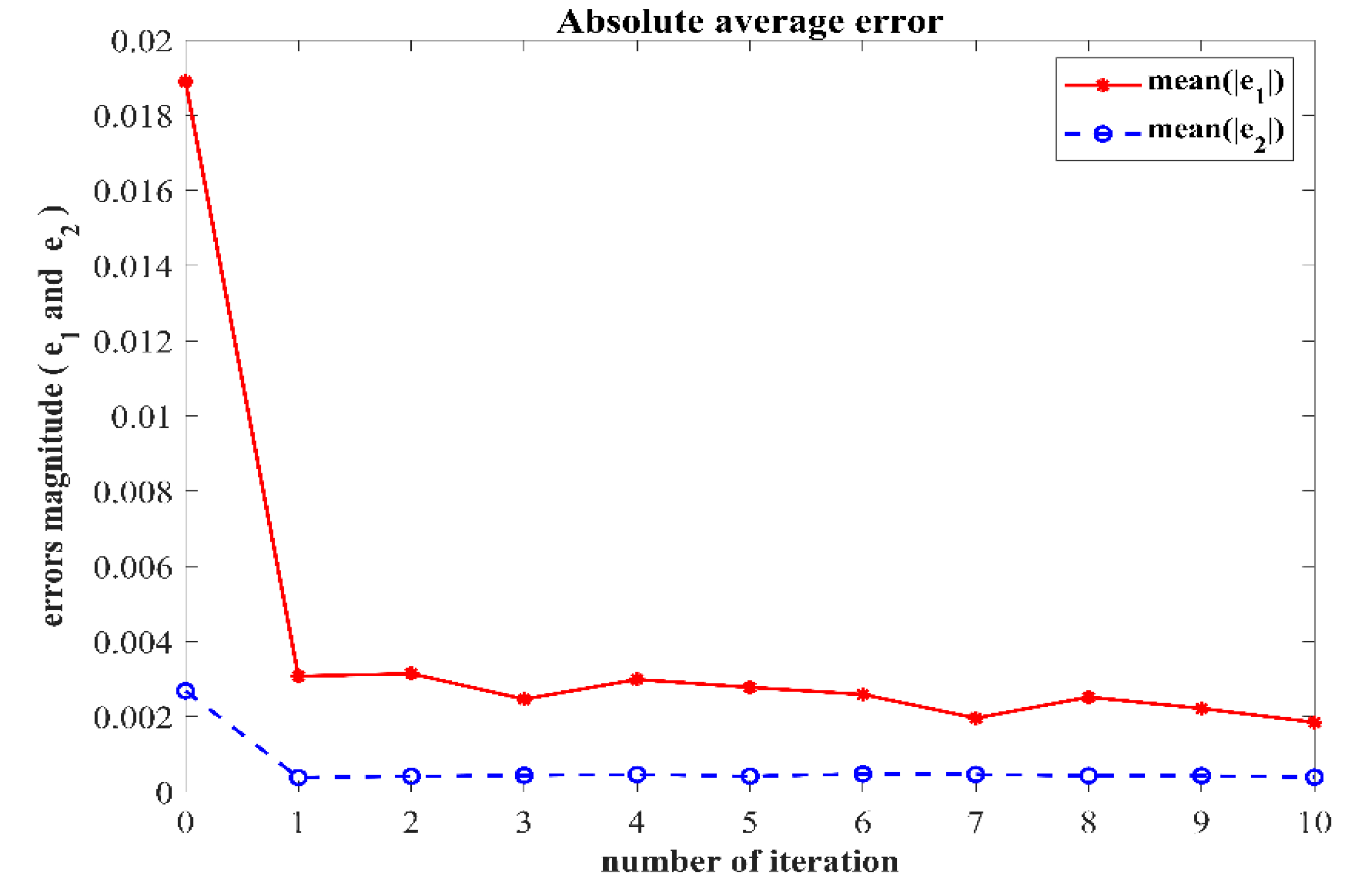
Based on the PD-type closed-loop iterative learning controller designed in this paper for numerical simulation, the trajectory tracking results of the first, third, fifth, seventh, and tenth iterations are shown in Figure 3, Figure 4, Figure 5, Figure 6 and Figure 7. Because the initial value of the iteration in each iterative learning process is randomly generated, the average value of the absolute value of the trajectory tracking error after the predefined time (called the average absolute error) was selected as the iterative convergence evaluation standard. The iterative convergence graph of the absolute average error and the number of iterations is shown in Figure 8.
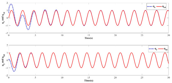
Figure 3.
Learning trajectory in the first iteration.
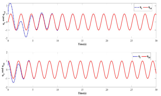
Figure 4.
Learning trajectory in the third iteration.
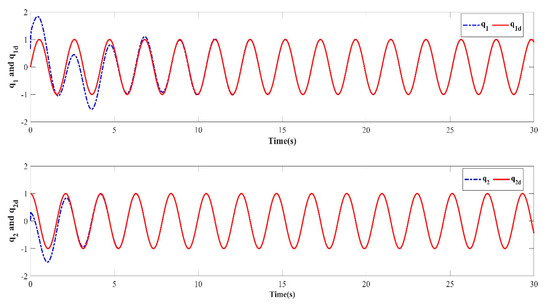
Figure 5.
Learning trajectory in the fifth iteration.
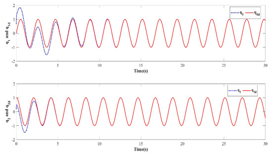
Figure 6.
Learning trajectory in the seventh iteration.
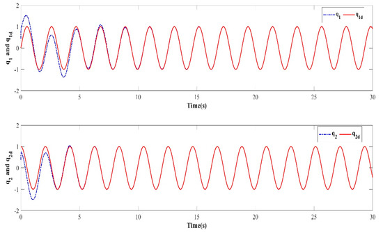
Figure 7.
Learning trajectory in the tenth iteration.
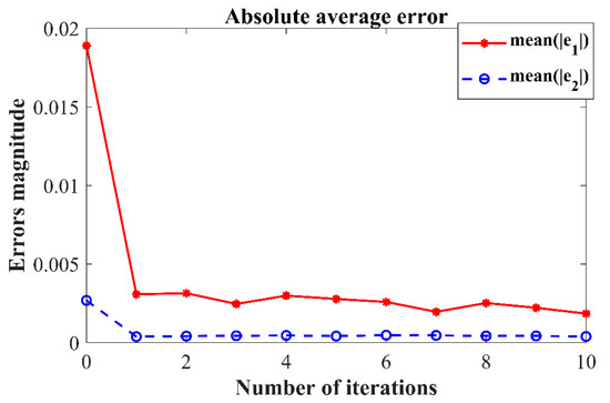
Figure 8.
Iterative error convergence trend.
The numerical simulation results show that in the simulation environment, where the initial values and were randomly generated in each iteration, based on the PD-type closed-loop iterative learning controller designed in this paper, the two degree of freedom manipulator system achieved iterative convergence after only two learning iterations. The absolute average error after 8s was lower than 0.004, which shows that, based on the control algorithm proposed in this paper, the end position of the manipulator can accurately track the desired trajectory after a predefined time, which verifies the feasibility of the algorithm. It effectively resolves the control problem such that the output of the nonlinear system can track the desired trajectory with high precision within the predefined time interval under an arbitrary initial value of iteration.
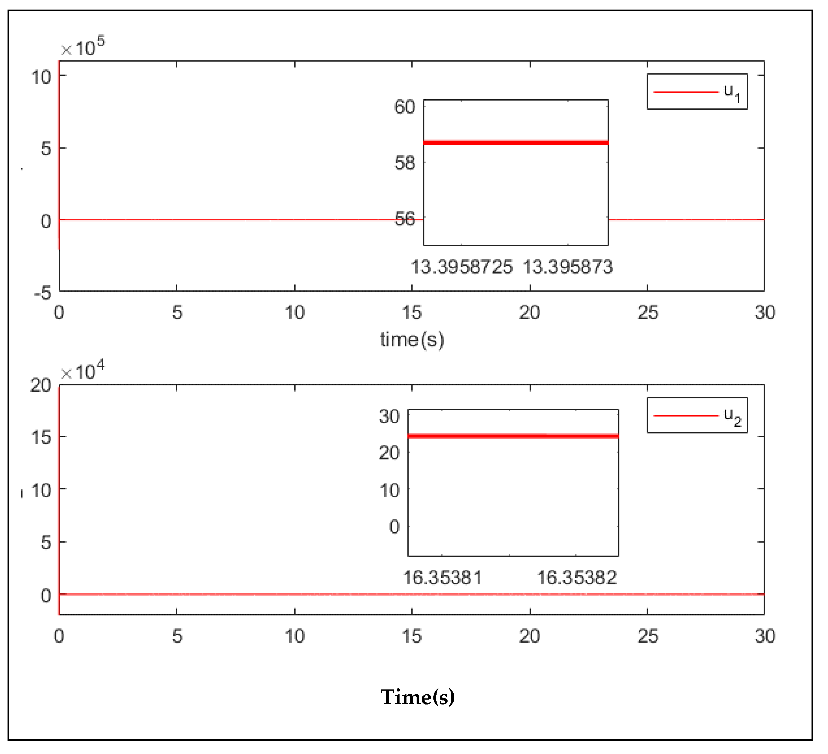
It can be seen from Figure 9 that the control torque of the manipulator was very large in the first few seconds, but that it then reduced to less than 60 N, while the value of u2 was even less than 30 N. This demonstrates that the proposed controller has smaller control input, which means the controller requires less effort from the manipulator.
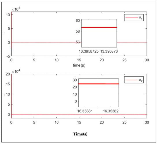
Figure 9.
Control input in the tenth iteration.
5.2. Case 2: Robustness (With Disturbances)
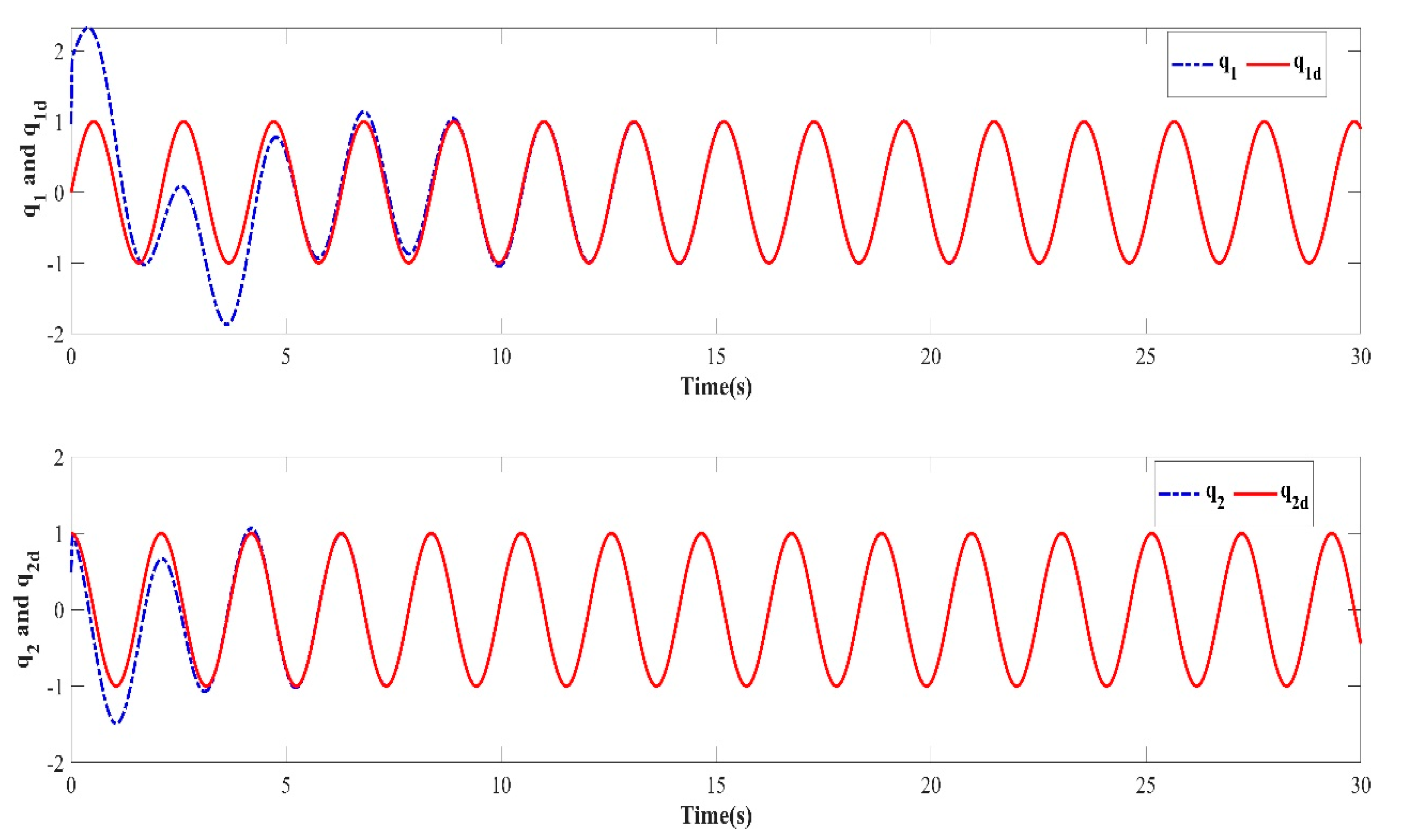
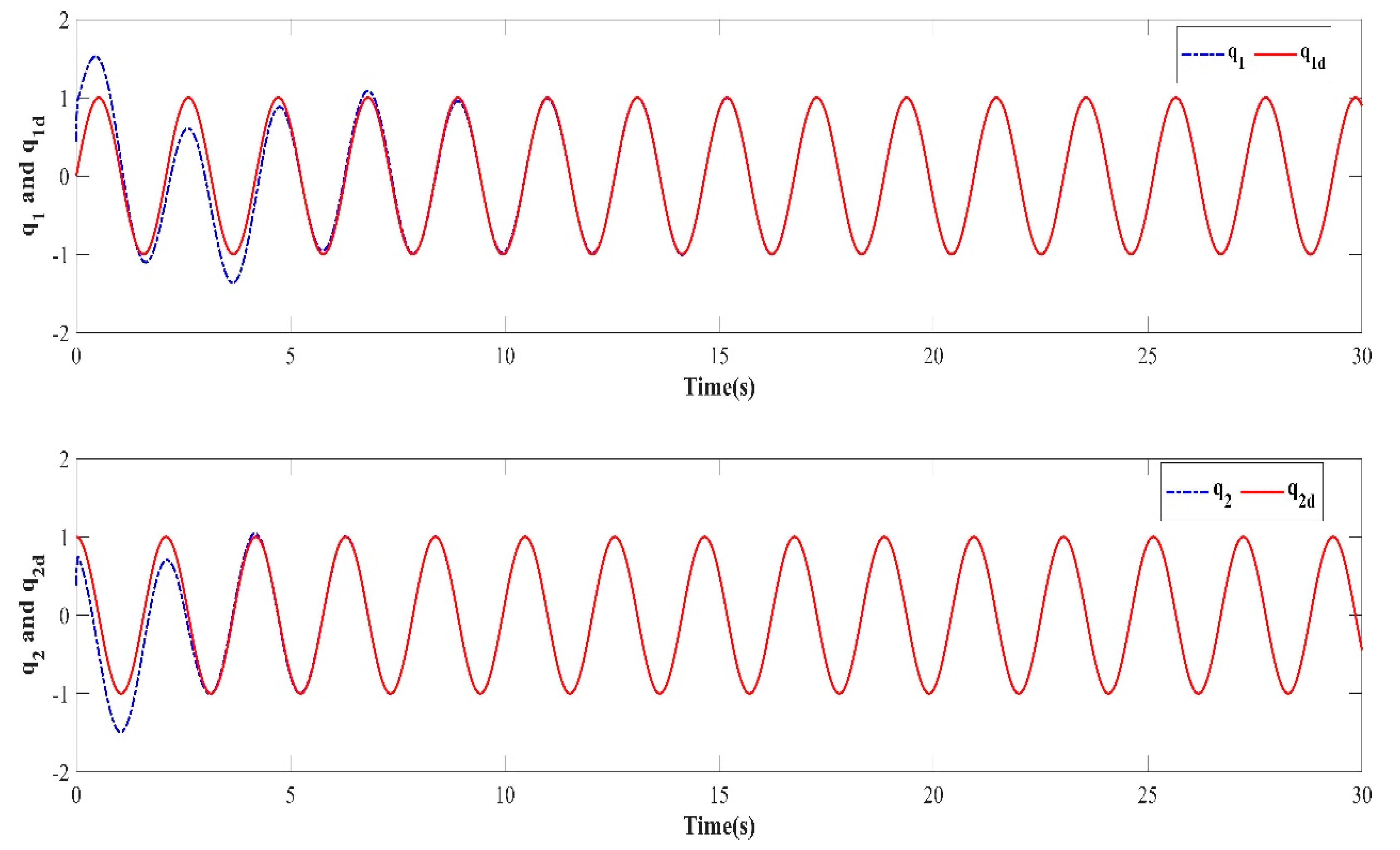
In order to verify the robustness of the controller to external disturbances while keeping the control parameters the same as in Case 1 and the initial value of the iteration in each iterative learning process randomly generated, a numerical simulation was performed after adding an external disturbance to the dynamic system of the two degree of freedom manipulator. The trajectory tracking effect after 10 iterations is shown in Figure 10. The iterative convergence diagram of the mean absolute error with respect to the number of iterations is shown in Figure 11.
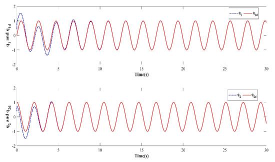
Figure 10.
Trajectory tracking effect of the tenth iteration.
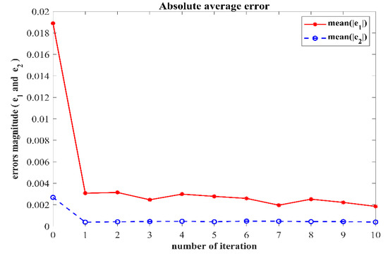
Figure 11.
Iterative convergence trend.
It can be seen from Figure 10 and Figure 11 that when an external disturbance was added to the dynamic system of the manipulator, the end position of the manipulator could still achieve high-precision tracking of the desired trajectory after the preset convergence time. By comparing Figure 7 with Figure 10, it can be seen clearly that after the external disturbance was added to the system, the absolute average error value and varying trend after the preset convergence time did not change. This indicates that the addition of an external disturbance to the mechanical arm dynamics system had no effect on the iterative convergence accuracy and convergence speed. The proposed controller was able to achieve high-precision trajectory tracking within the predefined time. It can therefore be concluded that the iterative learning control algorithm proposed in this paper is strongly robust in the face of bounded external disturbances.
6. Conclusions
This paper presented a study into the problem of accurate tracking control of a second-order nonlinear system with arbitrary iterative initial values within a preset time interval. First, a time-varying sliding mode surface with predefined-time convergence and zero initial value characteristics was constructed, and the Lyapunov stability criterion for predefined-time convergence, which is used to evaluate the trajectory tracking error in the sliding mode surface that can converge to the origin at the predefined-time, was given. Second, it was theoretically proven that the predefined convergence time was independent of the initial value of iteration and control parameters. Furthermore, in the process of designing an iterative learning controller, the iterative control problem of trajectory tracking under an arbitrary initial value of iteration was transformed into a time-varying sliding mode surface tracking iterative control problem when the initial iteration value is zero. This establishes a bridge for converting the theory of iterative learning control between the arbitrary initial value and the same initial value. Finally, we presented a design for a PD-type closed-loop iterative learning controller based on a time-varying sliding mode surface. It was proved theoretically that the trajectory tracking error of a second-order nonlinear system can converge and stabilize within the sliding mode surface after learning with a finite number of iterations. This confirmed that the system output was capable of accurately tracking the desired trajectory within a predefined time.
This work expands the application area of iterative learning control theory in practical engineering applications.
Author Contributions
Conceptualization and theoretical proof, C.-W.Y. and S.R.; formal analysis, S.R. funding acquisition, V.B., L.P. and S.M.; methodology, H.Z.; project administration, N.U.; resources, H.Z.; writing—original draft, C.-W.Y.; writing—review and editing, N.U., V.B. and S.M. All authors have read and agreed to the published version of the manuscript.
Funding
This work was supported in part by the Doctoral Grant Competition VSB—Technical University of Ostrava, under Grant CZ.02.2.69/0.0/0.0/19073/0016945; in part by the Operational Programme Research, Development and Education, under Project DGS/TEAM/2020-015; in part by the Partial Discharge Detection in Insulation Systems, National Centre for Energy, under Project TN01000007. This work also received partial support from Taif University Researchers Supporting Project number (TURSP-2020/144), Taif University, Taif, Saudi Arabia.
Institutional Review Board Statement
Not applicable.
Informed Consent Statement
Not applicable.
Data Availability Statement
Not applicable.
Acknowledgments
The authors acknowledge the support received from the Doctoral Grant Competition VSB—Technical University of Ostrava, under GrantCZ.02.2.69/0.0/0.0/19073/0016945; in part by the Operational Programme Research, Development and Education, under Project DGS/TEAM/2020-015; in part by the Partial Discharge Detection in Insulation Systems, National Centre for Energy, under Project TN01000007. This work also received partial support from Taif University Researchers Supporting Project number (TURSP-2020/144), Taif University, Taif, Saudi Arabia.
Conflicts of Interest
The authors declare no conflict of interest.
References
- Lee, J.H.; Lee, K.S. Iterative learning control applied to batch processes: An overview. Control Eng. Pract. 2007, 15, 1306–1318. [Google Scholar] [CrossRef]
- Li, G.; Lu, T.; Han, Y.; Xu, Z. Adaptive iterative learning control for high-order nonlinear systems with random initial state shifts. ISA Trans. 2022, 130, 205–215. [Google Scholar] [CrossRef] [PubMed]
- Sun, S.-T.; Li, X.-D. Quantized Iterative Learning Control for Nonlinear Switched Discrete-Time Systems with Actuator Saturation. In Proceedings of the 2022 IEEE 11th Data Driven Control and Learning Systems Conference (DDCLS), Chengdu, China, 3–5 August 2022; pp. 1297–1302. [Google Scholar]
- Cheng, X.; Jiang, H.; Shen, D.; Yu, X. A Novel Adaptive Gain Strategy for Stochastic Learning Control. IEEE Trans. Cybern. 2022. [Google Scholar] [CrossRef] [PubMed]
- Liu, T.; Ding, Y.; Wang, P.; Zhao, K.; Jia, J. Stability Control of Transport Robot Based on Iterative Learning Control. J. Phys. Conf. Ser. 2022, 2173, 012061. [Google Scholar] [CrossRef]
- Liu, J.; Jia, C. Direct and Indirect Technique Routes of Convergence Analysis for Discrete-time Iterative Learning Control. In Proceedings of the 2022 IEEE 11th Data Driven Control and Learning Systems Conference (DDCLS), Chengdu, China, 3–5 August 2022; pp. 899–903. [Google Scholar]
- Cheng, X.; Wang, H.; Wang, Q.; Feng, S. Rapid iterative learning algorithm of nonlinear time-delay system with initial deviation. Int. J. Electr. Eng. Educ. 2020, 0020720920940577. [Google Scholar] [CrossRef]
- Ma, F.; Li, C. Open-closed-loop PID-type iterative learning control for linear systems with initial state error. J. Vib. Control 2011, 17, 1791–1797. [Google Scholar]
- Riaz, S.; Lin, H.; Waqas, M.; Afzal, F.; Wang, K.; Saeed, N. An Accelerated Error Convergence Design Criterion and Implementation of Lebesgue-p Norm ILC Control Topology for Linear Position Control Systems. Math. Probl. Eng. 2021, 2021, 5975158. [Google Scholar] [CrossRef]
- Liu, F.; Zhang, K. PDα-Type Iterative Learning Control with Initial State Learning for Fractional-Order Systems. Xibei Gongye Daxue Xuebao/J. Northwestern Polytech. Univ. 2021, 39, 400–406. [Google Scholar] [CrossRef]
- Riaz, S.; Lin, H.; Akhter, M.P. Design and implementation of an accelerated error convergence criterion for norm optimal iterative learning controller. Electronics 2020, 9, 1766. [Google Scholar] [CrossRef]
- Yang, J.; Hang, M.; Lin, Y.; Zhang, Q. Adaptive state compensation using parameterized iterative learning control for periodic velocity ripple of permanent magnet linear motor. In Proceedings of the 2009 IEEE International Conference on Industrial Technology, Victoria, Australia, 10–13 February 2009. [Google Scholar]
- Riaz, S.; Lin, H.; Elahi, H. A novel fast error convergence approach for an optimal iterative learning controller. Iintegr. Ferroelectr. 2020, 213, 103–115. [Google Scholar] [CrossRef]
- Li, H.; Song, L.; Jiang, X.; Shi, H.; Su, C.; Li, P. Robust Model Predictive Control for Multi-phase Batch Processes with Asynchronous Switching. Int. J. Control Autom. Syst. 2022, 20, 84–98. [Google Scholar] [CrossRef]
- Sun, M.X.; Bi, H.B.; Zhou, G.L.; Wang, H.F. Feedback-aided PD-type Iterative Learning Control: Initial Condition Problem and Rectifying Strategies. Acta Autom. Sin. 2015, 41, 157–164. [Google Scholar]
- Lv, Q. Adaptive iterative learning control for inhibition effect of initial state random error. Zidonghua Xuebao/Acta Autom. Sin. 2015, 41, 1365–1372. [Google Scholar]
- Riaz, S.; Lin, H.; Mahsud, M.; Afzal, D.; Alsinai, A.; Cancan, M. An improved fast error convergence topology for PD α-type fractional-order ILC. J. Interdisciplinary Math. 2021, 24, 2005–2019. [Google Scholar] [CrossRef]
- Yan, Q.Z.; Sun, M.X.; Cai, J.P. Reference-signal Rectifying Method of Iterative Learning Control. Acta Autom. Sin. 2017, 43, 1470–1477. [Google Scholar]
- Chien, C.J.; Hsu, C.T.; Yao, C.Y. Fuzzy system-based adaptive iterative learning control for nonlinear plants with initial state errors. IEEE Trans. Fuzzy Syst. 2004, 12, 724–732. [Google Scholar] [CrossRef]
- Sun, M.; Wu, T.; Chen, L.; Zhang, G. Neural AILC for Error Tracking Against Arbitrary Initial Shifts. IEEE Trans. Neural Netw. Learn. Syst. 2017, 29, 2705–2716. [Google Scholar] [CrossRef] [PubMed]
- Sun, M.X.; Huang, B.J.; Zhang, X.Z. PD-type iterative learning control for a class of uncertain time-delay systems with arbitrary initial states. Control Theory Appl. 1998, 6, 853–858. [Google Scholar]
- Liu, Y.; Niu, Y. Sliding mode control for uncertain switched systems subject to state and input delays. Trans. Inst. Meas. Contr. 2018, 40, 3232–3238. [Google Scholar] [CrossRef]
Disclaimer/Publisher’s Note: The statements, opinions and data contained in all publications are solely those of the individual author(s) and contributor(s) and not of MDPI and/or the editor(s). MDPI and/or the editor(s) disclaim responsibility for any injury to people or property resulting from any ideas, methods, instructions or products referred to in the content. |
© 2022 by the authors. Licensee MDPI, Basel, Switzerland. This article is an open access article distributed under the terms and conditions of the Creative Commons Attribution (CC BY) license (https://creativecommons.org/licenses/by/4.0/).


