The proposed availability optimization decision support design system in this study attempts to consider the component redundancy number, failure rate, and repair rate in order to decide on an appropriate repairable n-stage mixed system, in which different combinations of subsystems, such as single component, parallel, standby, and k-out-of-q, are connected in series configuration. The enumeration method, the tabu search method, the simulated annealing approach, the non-equilibrium simulated annealing approach, and the modified redundancy allocation heuristic method combined with the modified genetic algorithm will be conducted to run different simulation cases regarding different system configurations and system constraint requirements.
For the five proposed ENUM-MGA, TS–MGA, SA–MGA, NESA–MGA, and MRAH–MGA combined methods, the modified genetic algorithm is adopted to acquire the optimal component repair rates and the optimal component failure rates for all subsystems jointly in the second stage, depending on the redundant component amount determined by ENUM, TS, SA, NESA, and MRAH in the first stage. Before implementing the following simulation cases, the parameter design for the modified genetic algorithm will be conducted first. According to the results of several trial and error tests, it will mostly ameliorate the quality of first final converged solution and the converged time by utilizing a chromosome crossover rate equal to 0.95, a chromosome mutation rate equal to 0.5, a chromosome population equal to 200, and a genetic generation equal to 200 in the five proposed ENUM-MGA, TS–MGA, SA–MGA, NESA–MGA, and MRAH–MGA combined methods for most simulation cases.
4.2. The Simulation Case for n-Stage Standby System
Since the
n-stage single component series system assumes all subsystems comprise one single component, the proposed availability optimization decision support design system can only allocate the component failure rate and the component repair rate for each subsystem to achieve the system availability optimization design. However, this kind of system configuration has some disadvantages in reaching the certain level of the system availability requirement. The main disadvantage is that, because all the series connected subsystems only have one single component, the failure of one component would cause the entire system to shut down in order to conduct the repair operation. Furthermore, the system shutdown will result in a huge operation loss cost during the repair. To avoid this kind of system shutdown, the component reliability and component maintainability need to be enhanced dramatically, but it will also cost a lot to meet the high level of the system availability requirement due to technical difficulty. Therefore, the proposed availability optimization decision support design system intends to apply component redundancy to reach the high level of the system availability requirement with less cost. In the sequel, this study will further conduct the simulation cases by the ENUM-MGA, TS–MGA, SA–MGA, NESA–MGA, and MRAH–MGA combined methods for the
n-stage standby system, which assumes all subsystems are standby configurations and are connected in series structure.
Table 5 and
Table 6 show the simulation results produced by the ENUM–MGA combined method.
Table 7 and
Table 8 display the simulation results produced by the TS–MGA combined method.
Table 9 and
Table 10 demonstrate the simulation results produced by the SA–MGA combined method.
Table 11 and
Table 12 show the simulation results produced by the NESA–MGA combined method.
Table 13 and
Table 14 display the simulation results produced by the MRAH–MGA combined method.
Regarding the simulation case of the
n-stage standby system, the simulation outcomes obtained by the ENUM-MGA combined method are displayed in
Table 4 and
Table 6.
Table 5 demonstrates the total system costs of 20 simulation runs, the related average total system cost equal to 244.02545, and the related lowest total system cost equal to 243.209.
Table 5 displays the optimal redundancy amounts, the optimal failure rates, the optimal repair rates, availabilities for all subsystems, the optimal total system cost, and the optimal system availability for the principal simulation case of the
n-stage standby system. Furthermore, the convergence graphs in the following
Figure 3 show that the total system cost can be easily improved and converged to the lowest 243.209 with the average CPU running time of 2669.9273 s for the principle
n-stage standby system by adopting the proposed ENUM–GA combined method.
According to the results of
Table 3,
Table 4,
Table 5 and
Table 6, the optimal total system cost obtained by the ENUM-MGA combined method for the
n-stage standby system is much better than the optimal total system cost obtained by the genetic algorithm for the
n-stage single component series system. Moreover, the following additional simulation results conducted by the TS–MGA, SA–MGA, NESA–MGA and MRAH–MGA combined methods for the
n-stage standby system obviously show that the proposed availability optimization decision support design system can use the component redundancy design to save a lot of cost and meet the high level of the system availability requirement compared to the
n-stage single component series system.
Table 7.
The total system costs of 28 simulation runs obtained by TS–MGA for the n-stage standby system.
Table 7.
The total system costs of 28 simulation runs obtained by TS–MGA for the n-stage standby system.
| cr-rate = 0.95 mu-rate = 0.5 GApopulation = 200 GAloop = 200 |
|---|
| Total System Cost (TabuLoop) (CPU Time) |
|---|
| 243.63(50)(1983.4) | 242.57(50)(1912.2) | 240.86(100)(3949.1) | 240.4(100)(3861.67) | 237.5(150)(5820.4) |
| 238.27(150)(5752.2) | 238.552(200)(7769) | 237.988(200)(7817.9) | 237.983(200)(7640) | 237.838(200)(7648) |
| 237.751(200)(7751) | 237.654(200)(7644) | 237.587(200)(7645.8) | 237.529(200)(7721.7) | 237.4(200)(7584.3) |
| 237.396(200)(7624) | 237.396(200)(7638) | 237.36(200)(7777) | 237.306(200)(7672) | 237.299(200)(8126) |
| 237.291(200)(7795) | 237.272(200)(7740.6) | 237.262(200)(7726) | 237.012(200)(7911) | 236.951(200)(7696) |
| 236.831*(200)(7641) | 237(250)(9435.22) | 236.97(250)(9555.29) | | |
Lowest Total System Cost (TabuLoop) (CPUTime) 236.831*(200)(7641)
Avg. Total System Cost (TabuLoop) (Avg. CPU Time) |
| 243.1(50)(1947.8) | 240.6(100)(3905.4) | 237.88(150)(5786.3) | 237.48(200)(7728.42) | 36.99(250)(9495.25) |
By conducting the TS–MGA combined method for the principal
n-stage standby system,
Table 7 above shows 28 selected simulated results of the total system costs by setting TabuLoop equal to 50 with an average CPU running time of 1947.8 s until 250 with an average CPU running time of 9495.25 s, and it further converges the average total system cost of 243.1 to 236.99 and the total system cost of 243.63 to the lowest 236.831. Since the average total system cost of 237.48 with 200 Tabu loops is a little higher than 236.99 with 250 Tabu loops, and, moreover, the lowest converged total system cost happened at 200 Tabu loops, the simulation process stops running at 200 Tabu loops and finally reaches the lowest converged result of 236.831. Furthermore, for the above lowest converged result of 236.831, which is obtained at 200 Tabu loops,
Figure 4 shows that the total system cost and the average total system cost have improved and converged for the principle
n-stage standby system by applying the proposed TS–GA combined method.
Table 8 displays the optimal system cost related to the optimal failure rates, the optimal repair rates, the availability of all subsystems, and the system availability, as follows:
Table 8.
Optimal Solutions obtained by TS–MGA for the n-stage standby system.
Table 8.
Optimal Solutions obtained by TS–MGA for the n-stage standby system.
| TabuLoop = 200 cr-rate = 0.95 mu-rate = 0.5 GApopulation = 200 GAloop = 200 |
|---|
| Decision Variables | Subsystem(i) |
|---|
| | 1 | 2 | 3 | 4 | 5 |
|---|
| 3 | 3 | 2 | 3 | 2 |
| (10−3) | 0.3261 | 0.2749 | 0.1507 | 0.5963 | 0.2555 |
| 0.0012 | 0.0010 | 0.0010 | 0.0017 | 0.0015 |
| 0.9852 | 0.9838 | 0.9808 | 0.9710 | 0.9750 |
| Optimal Total System Cost 236.831 |
| 0.9000 |
Table 9.
The total system costs of 20 simulation runs obtained by SA–GA for the n-stage standby system.
Table 9.
The total system costs of 20 simulation runs obtained by SA–GA for the n-stage standby system.
| cr-rate = 0.95 mu-rate = 0.5 GApopulation = 200 GAloop = 200 |
|---|
| Total System Cost (SAloop) (CPU Time) |
|---|
| 244.11(50)(4403.51) | 243.35(50)(4197.83) | 243.07(50)(4204.29) | 242.844(50)(4358.55) | 242.44(50)(4768) |
| 238.693(50)(4418.54) | 241(100)(8680) | 240.75(100)(8609.14) | 237.89(100)(8817.26) | 238.50(150)(12,605) |
| 237.11(150)(12,422) | 239.08(200)(17,081) | 237.13(200)(16,711) | 238.87(250)(21,676) | 236.46*(250)(21,233) |
| 237.02(400)(22,524) | 237.01(400)(22,061.8) | 236.86(400)(22,088) | 236.77(500)(47,528.5) | 236.76(500)(46,295) |
| Lowest Total System Cost (SAloop)(CPUTime) 236.46*(250)(21,232.93) |
| Avg. Total System Cost (SAloop) (Avg. CPUTime) |
| 242.4(50)(4391.8) | 239.88(100)(8702.2) | 237.8(150)(12,513.5) | 238.1(200)(16,896.14) | 236.97(400)(22,224.54) |
| 236.766(500)(46,911.73) | | | | |
By conducting the SA–MGA combined method for the principal
n-stage standby system,
Table 9 above shows 20 selected simulated results of the total system costs by setting SAloop equal to 50 with an average CPU running time of 4391.8 s until 400 with an average CPU running time of 22,224.54 s, and it further converges the average total system cost of 242.4 to 236.97 and the total system cost of 244.11 to the lowest 236.46. Since the average total system cost of 236.97 with 400 SA loops is a little higher than 236.766 with 500 SA loops, but with around half of the CPU running time, the simulation process stops running at 400 SA loops and finally reaches the lowest converged result of 236.46. Moreover,
Figure 5 also displays that the average total system cost and the total system cost have improved and converged for the principal
n-stage standby system by adopting the proposed SA–GA combined method.
For the above lowest converged result of 236.46, which is obtained at 250 SA loops,
Table 10 displays the optimal system cost related to the optimal failure rates, the optimal repair rates, the availability of all subsystems, and the system availability, as follows:
Table 10.
Optimal Solutions obtained by SA–MGA for the n-stage standby system.
Table 10.
Optimal Solutions obtained by SA–MGA for the n-stage standby system.
| SAloop = 250, cr-rate = 0.95, mu-rate = 0.5, GApopulation = 200, GAloop = 200 |
|---|
| Decision Variables | Subsystem(i) |
|---|
| | 1 | 2 | 3 | 4 | 5 |
|---|
| 3 | 3 | 2 | 3 | 2 |
| (10−3) | 0.3325 | 0.2738 | 0.1401 | 0.6057 | 0.2560 |
| 0.0011 | 0.0010 | 0.0010 | 0.0017 | 0.0015 |
| 0.9823 | 0.9852 | 0.9818 | 0.9718 | 0.9747 |
| Optimal Total System Cost 236.46 |
| 0.9000 |
Table 11.
The total system costs of 20 simulation runs obtained by NESA–MGA for the n-stage standby system.
Table 11.
The total system costs of 20 simulation runs obtained by NESA–MGA for the n-stage standby system.
| InLoop = 10, cr-rate = 0.95, mu-rate = 0.5, GApopulation = 200, GAloop = 200 |
|---|
| Total System Cost (NESAloop) (CPU Time) |
|---|
| 238.953(50)(871) | 237.815(50)(879.4) | 238.456(50)(956.6) | 238.298(100)(1840.4) | 237.94(100)(1990.4) |
| 237.98(150)(2830) | 237.83(150)(2736) | 237.63(200)(3832) | 237.76(200)(3869.33) | 237.36(250)(4552.24) |
| 237.41(250)(4592.9) | 237.58(250)(4517.4) | 237.396(250)(4603) | 237.8(400)(7029.45) | 237.62(400)(7974.95) |
| 237.59(400)(7405.6) | 237.35(500)(9305.5) | 237.27(500)(9441.5) | 237.57(600)(11,486.7) | 237.57(600)(11,339.5) |
| Lowest Total System Cost (NESAloop) (CPU Time) 237.27*(500)(9441.5) |
| Avg. Total System Cost (NESAloop) (Avg. CPU Time) |
| | 238.408(50)(902) | 238.12(100)(1915) | 237.9(150)(2783.2) | 237.69(200)(3851) |
| | 237.44(250)(4566.45) | 237.67(400)(7470) | 237.31(500)(9373.45) | 237.57(600)(11,413) |
By conducting the NESA–MGA combined method regarding the principal
n-stage standby system,
Table 11 above shows 20 selected simulated results of the total system costs by setting NESAloop equal to 50 with an average CPU running time of 902 s until 500 with an average CPU running time of 9373.45 s, and it further converges the average total system cost of 238.408 to 237.31 and the total system cost of 238.953 to the lowest 237.31. Since the average total system cost of 237.31 with 500 NESA loops is lower than 237.57 with 600 NESA loops, the simulation process stops running at 500 NESA loops and finally reaches lowest converged result of 237.27. Therefore,
Figure 6 also clearly illustrates that the average total system cost and the total system cost have improved and at last converged for the principal
n-stage standby system by adopting the proposed NESA–MGA combined method.
Additionally, for the lowest converged result of 237.27,
Table 12 illustrates the optimal system cost associated with the optimal failure rates, the optimal repair rates, the availability of all subsystems, and the system availability.
Table 12.
Optimal Solutions obtained by NESA–MGA for the n-stage standby system.
Table 12.
Optimal Solutions obtained by NESA–MGA for the n-stage standby system.
| NESAloop = 500 InLoop = 10 cr-rate = 0.95 mu-rate = 0.5 GApopulation = 200 GAloop = 200 |
|---|
| Decision Variables | Subsystem(i) |
|---|
| | 1 | 2 | 3 | 4 | 5 |
|---|
| 2 | 3 | 2 | 3 | 3 |
| (10−3) | 0.2786 | 0.2873 | 0.1411 | 0.5643 | 0.3147 |
| 0.0016 | 0.0010 | 0.0010 | 0.0018 | 0.0010 |
| 0.9759 | 0.9809 | 0.9812 | 0.9776 | 0.9802 |
| Optimal Total System Cost 237.27 |
| 0.9000 |
In
Table 12 and
Table 14, the simulation results obtained by the MRAH -MGA combined method display the total system costs of 20 simulation runs, the related average total system cost equal to 237.807, and the lowest total system cost equal to 226.450, which is superior to all other combined methods and has an extremely low average CPU running time of around 89 s.
Table 13.
The total system costs of 20 simulation runs obtained by MAHA–MGA for the n-stage standby system.
Table 13.
The total system costs of 20 simulation runs obtained by MAHA–MGA for the n-stage standby system.
| cr-rate = 0.95 mu-rate = 0.5 GApopulation = 200 GAloop = 200 |
|---|
| Total System Cost (Running Time) |
|---|
| 238.067(90.18) | 237.87(90.21) | 239.598(91.55) | 238.514(86.33) | 238.916(90.19) | 238.53(88.33) | 241.376(91.44) |
| 236.094(89.25) | 237.921(90.24) | 238.342(91.67) | 238.875(96.67) | 238.603(97.45) | 235.253(97) | 235.74(96.6) |
| 239.891(98) | 239.066(97.4) | 239.607(98.4) | 238.037(96.7) | 239.392(97.4) | 226.450*(5.31) | |
| Lowest Total System Cost (CPU Time) 226.450*(5.31) |
| Avg. Total System Cost (Avg. CPU Time) 237.807(89.0277) |
Table 14.
Optimal Solutions obtained by MAHA–MGA for the n-stage standby system.
Table 14.
Optimal Solutions obtained by MAHA–MGA for the n-stage standby system.
| Decision Variables | Subsystem(i) |
|---|
| | 1 | 2 | 3 | 4 | 5 |
|---|
| 2 | 2 | 2 | 3 | 3 |
| (10−3) | 0.3886 | 0.2331 | 0.1960 | 0.7868 | 0.4314 |
| 0.0024 | 0.0012 | 0.0013 | 0.0017 | 0.0012 |
| 0.9484 | 0.9796 | 0.9907 | 0.9866 | 0.9948 |
| Optimal Total System Cost 226.450 |
| 0.90335 |
Moreover, the following
Figure 7 remarkably demonstrates that the total system cost has been ameliorated and, in the end, converged for the principle
n-stage standby system by conducting the proposed MRAH–MGA combined method.
4.3. The Simulation Case for Parallel-Series System
Besides the
n-stage standby system, the parallel-series system can also be applied to take advantage of component redundancy to reach the high level of the system availability requirement with less cost. The proposed availability optimization decision support design system will further conduct the simulation cases by the ENUM-MGA, TS–MGA, SA–MGA, NESA–MGA, and MAHA–MGA combined methods for the parallel-series system, which assumes all subsystems are parallel configurations and are connected in series structure.
Table 15 and
Table 16 show the simulation results produced by the ENUM–MGA combined method.
Table 17 and
Table 18 display the simulation results produced by the TA–MGA combined method.
Table 19 and
Table 20 demonstrate the simulation results produced by the SA–MGA combined method.
Table 21 and
Table 22 show the simulation results produced by the NESA–MGA combined method.
Table 23 and
Table 24 display the simulation results produced by the MAHA–MGA combined method.
For the simulation case of the parallel-series system, the simulation results obtained by the ENUM-MGA combined method is expressed in
Table 14 and
Table 16 and
Figure 8.
Table 15 shows the total system costs of 20 simulation runs, the related average total system cost of 221.245, and the related lowest total system cost of 220.278. The convergence graphs in
Figure 8 distinctly illustrate that the total system cost can likely be improved and converged for the principal parallel-series system by implementing the proposed ENUM–MGA combined method.
Furthermore,
Table 15 demonstrates the optimal system cost, the optimal failure rates, the optimal repair rates, the availabilities for all subsystems, and the system availability for the principal simulation case of the parallel-series system. In
Table 16, the optimal total system cost obtained by the ENUM-MGA combined method for the parallel-series system is much better than the optimal total system cost obtained by the genetic algorithm for the
n-stage single component series system in
Table 6. Moreover, other simulation results produced by the TS–MGA, SA–MGA, NESA–MGA, and MRAH–MGA combined methods for the parallel-series system also show that the proposed availability optimization decision support design system can apply the component redundancy design of the parallel-series system to decrease a lot of the cost and meet the high level of the system availability requirement compared to the
n-stage single component series system.
Table 17.
The total system costs of 32 simulation runs obtained by TA–MGA for the parallel-series system.
Table 17.
The total system costs of 32 simulation runs obtained by TA–MGA for the parallel-series system.
| cr-rate = 0.95 mu-rate = 0.5 GApopulation = 200 GAloop = 200 |
|---|
| Total System Cost (TabuLoop) (CPU Time) |
|---|
| 222.42(50)(1894.79) | 221.92(50)(1966.3) | 220.05(50)(1873.5) | 218(100)(3791.59) | 216.825(100)(3799) |
| 216.59(100)(3787.9) | 216.64(150)(5670.7) | 215.69(150)(5760) | 215.51(150)(5656.5) | 215.17(200)(7409.4) |
| 215.169(200)(7426.8) | 215.167(200)(7364.7) | 215.15(200)(7787.3) | 215.14(200)(7363) | 215.13(200)(7440.6) |
| 215.1(200)(7405.4) | 215.09(200)(7432.3) | 215.086(200)(7537.2) | 215.064(200)(7345.14) | 214.993(200)(7394.4) |
| 214.972(200)(7802) | 214.972(200)(7621.7) | 214.957(200)(7374.8) | 214.91(200)(7439.5) | 214.88(200)(7470.98) |
| 214.823(200)(7336) | 214.779(200)(7455) | 214.74(200)(7497.28) | 214.74(200)(7425.56) | 214.985(250)(9484.38) |
| 214.69(250)(9350.25) | 214.62*(250)(9361) | | | |
| Lowest Total System Cost (TabuLoop)(CPU Time) 214.62*(250)(9361) |
| Avg. Total System Cost (TabuLoop) (Avg. CPUTime) |
| 221.46(50)(1911.5) | 217.14(100)(3793) | 215(200)(7468.7) | 214.765(250)(9398.55) | |
By applying the TS–MGA combined method for the principal parallel-series system,
Table 17 above shows 32 selected simulated outcomes of the total system costs by assuming TabuLoop equal to 50 with an average CPU running time of 1911.5 s until 250 with an average CPU running time of 9398.55 s, and it further converges the average total system cost from 221.46 to 214.765 and the total system cost of 222.42 to the lowest 214.62. Since the average total system cost of 215 with 200 Tabu loops is just a little higher than 214.765 with 250 Tabu loops, the simulation process stops running at 250 Tabu loops and finally achieves the lowest converged result of 214.62.
Figure 9 demonstrates that the total system cost and the average total system cost have improved and converged for the principal parallel-series system by adopting the proposed TS–MGA combined method.
Additionally, for the above-mentioned lowest converged total system cost of 214.62, which is obtained at 250 Tabu loops,
Table 18 displays the optimal system cost related to the optimal failure rates, the optimal repair rates, the availability of all subsystems, and the system availability, as follows:
Table 18.
Optimal Solutions obtained by TA–MGA for the parallel-series system.
Table 18.
Optimal Solutions obtained by TA–MGA for the parallel-series system.
| TabuLoop = 250 cr-rate = 0.95 mu-rate = 0.5 GApopulation = 200 GAloop = 200 |
|---|
| Decision Variables | Subsystem(i) |
|---|
| | 1 | 2 | 3 | 4 | 5 |
|---|
| 3 | 3 | 2 | 3 | 2 |
| (10−3) | 0.3688 | 0.2925 | 0.1429 | 0.6483 | 0.2609 |
| 0.0010 | 0.0009 | 0.0009 | 0.0015 | 0.0014 |
| 0.9808 | 0.9838 | 0.9816 | 0.9730 | 0.9766 |
| Optimal Total System Cost 214.62 |
| 0.9000 |
By adopting the SA–MGA combined method to implement the simulation runs for the parallel-series system, the following
Table 19 displays 20 selected simulated results of the total system costs by assuming SAloop equal to 50 with an average CPU running time of 4175.08 s until 150 with an average CPU running time of 12,235.82 s, and it further converges the average total system cost of 220.6968 to 215.80295 and the total system cost of 222.13 to the lowest 214.7569. Because the average total system cost of 215.80295 with 150 SA loops is higher than 215.7916 with 100 SA loops, the simulation process can certainly stop running at 100 SA loops and converge to the lowest result of 214.7569.
Table 19.
The total system costs of 20 simulation runs obtained by SA–MGA for the parallel-series system.
Table 19.
The total system costs of 20 simulation runs obtained by SA–MGA for the parallel-series system.
| cr-rate = 0.95 mu-rate = 0.5 GApopulation = 200 GAloop = 200 |
|---|
| Total System Cost (SAloop) (CPU Time) |
|---|
| 222.13(50)(4181.43) | 220.93(50)(4194.25) | 219.025(50)(4149.57) | 217.15(100)(8355.43) |
| 216.7015(100)(8194.88) | 216.7011(100)(8157.18) | 216.69(100)(8143.85) | 216.135(100)(8144.83) |
| 216.11(100)(8105.175) | 215.825(100)(8155.55) | 215.59(100)(8169.5) | 215.54(100)(8179.6) |
| 215.45(100)(8345.35) | 215.14(100)(8187.4) | 215.11(100)(8179.3) | 215.02(100)(8171.8) |
| 214.95(100)(8166.9) | 214.7569*(100)(8182.35) | 215.9081(150)(12,510.3) | 215.6978(150)(12,235.8) |
| Lowest Total System Cost (SAloop)(CPUTime) 214.7569*(100)(8182.35) |
| Avg. Total System Cost (SAloop)(CPUTime) |
| 220.6968(50)(4175.08) | 215.7916*(100)(8182.2) | 215.80295(150)(12,235.81699) | |
In the following,
Figure 10 displays that the total system cost and the average total system cost have improved and converged for the principal parallel-series system by employing the proposed SA–MGA combined method.
Furthermore, for the above lowest converged result of 214.7569, which is obtained at 100 SA loops,
Table 20 shows the optimal system cost related to the optimal failure rate, the optimal repair rate, the availability of each subsystem, and the system availability, as follows:
Table 20.
Optimal Solutions obtained by SA–MGA for the parallel-series system.
Table 20.
Optimal Solutions obtained by SA–MGA for the parallel-series system.
| SAloop = 100 cr-rate = 0.95 mu-rate = 0.5 GApopulation = 200 GAloop = 200 |
|---|
| Decision Variables | Subsystem(i) |
|---|
| | 1 | 2 | 3 | 4 | 5 |
|---|
| 3 | 3 | 2 | 3 | 2 |
| (10−3) | 0.3552 | 0.2914 | 0.1431 | 0.6854 | 0.2495 |
| 0.0010 | 0.0009 | 0.0010 | 0.0015 | 0.0014 |
| 0.9810 | 0.9843 | 0.9853 | 0.9685 | 0.9768 |
| Optimal Total System Cost 214.7569 |
| 0.9000 |
By utilizing the NESA–MGA combined method to conduct the simulation cases for the parallel-series system, the following
Table 21 displays 22 selected simulated results of the total system costs by assuming NESAloop equal to 50 with an average CPU running time of 493.3975588 s until 1000 with an average CPU running time of 12,787.95585 s, and it further converges the average total system cost of 218.12722 to 215.3146 and the total system cost of 218.9289 to the lowest 214.9928. Since the average total system cost of 216.01448 with 300 NESA loops is just a little higher than 215.3146 with 1000 NESA loops, the simulation process ceases running at 1000 NESA loops and finally reaches the lowest converged result of 214.9928.
Table 21.
The total system costs of 20 simulation runs obtained by NESA–MGA for the parallel-series system.
Table 21.
The total system costs of 20 simulation runs obtained by NESA–MGA for the parallel-series system.
| InLoop = 10 cr-rate = 0.95 mu-rate = 0.5 GApopulation = 200 GAloop = 200 |
|---|
| Total System Cost (NESAloop) (CPU Time) |
|---|
| 218.9289(50)(488.32) | 218.7698(50)(495.24) | 218.3487(50)(495.17) | 218.087(50)(478.486) | 216.502(50)(509.77) |
| 218.06(100)(996.86) | 217.459(100)(951) | 217.274(100)(941.2) | 217.24(100)(942.9) | 216.11(100)(968.27) |
| 217.45(200)(1988.4) | 216.87(200)(1966.1) | 216.85(200)(1892) | 216.48(200)(2000) | 215.7231(200)(1998.7) |
| 216.3836(300)(3047) | 216.0787(300)(3059.9) | 216.0624(300)(2890) | 216.0151(300)(2845.8) | 215.5326(300)(2894) |
| 215.6364(1000)(12,711.696) | 214.9928*(1000)(12,864.215) | | | |
| Avg. Total System Cost(NESAloop)(CPUTime) |
| 218.12722(50)(493.3975588) | 217.22942(100)(960.0457) | 216.6767(200)(1969.03851) | 216.01448(300)(2947.507125) | 215.3146(1000)(12,787.95585) |
| Lowest Total System Cost (NESAloop)(CPUTime)214.9928*(1000)(12,864.215) |
In the following,
Figure 11 illustrates that the total system cost and the average system cost have improved and converged for the principle parallel-series system by introducing the proposed NESA–MGA combined method.
Furthermore, for the lowest converged result of 214.9928,
Table 22 illustrates the optimal system cost associated with the optimal failure rates, the optimal repair rates, the availability of all subsystems, and the system availability.
Table 22.
Optimal Solutions obtained by NESA–MGA for the parallel-series system.
Table 22.
Optimal Solutions obtained by NESA–MGA for the parallel-series system.
| NESAloop = 1000 InLoop = 10 cr-rate = 0.95 mu-rate = 0.5 GApopulation = 200 GAloop = 200 |
|---|
| Decision Variables | Subsystem(i) |
|---|
| | 1 | 2 | 3 | 4 | 5 |
|---|
| 3 | 3 | 2 | 3 | 2 |
| (10−3) | 0.3584 | 0.295 | 0.1303 | 0.6676 | 0.2533 |
| 0.0010 | 0.0009 | 0.0009 | 0.0014 | 0.0015 |
| 0.9796 | 0.9843 | 0.9851 | 0.9680 | 0.9789 |
| Optimal Total System Cost 214.9928 |
| 0.9000 |
Table 22 and
Table 24 display the simulation consequences acquired by the MAHA-MGA combined method for the total system costs of 20 simulation runs, the related average total system cost equal to 215.7925, and the lowest total system cost equal to 208.9659, which is superior to all other combined methods and has an extremely low average CPU running time of around 88.455 s.
Table 23.
The total system costs of 20 simulation runs obtained by MRAH–MGA for the parallel-series system.
Table 23.
The total system costs of 20 simulation runs obtained by MRAH–MGA for the parallel-series system.
| cr-rate = 0.95 mu-rate = 0.5 GApopulation = 200 GAloop = 200 |
|---|
| Total System Cost (CPU Time) |
|---|
| 218.4072(88.5) | 218.2744(87.895) | 218.0376(87.42) | 217.6616(90.248) | 217.5924(90.046) | 216.8774(89.3642) |
| 216.1849(89.5495) | 216.0018(87.3153) | 215.9571(85.0562) | 215.9565(91.17) | 215.7456(85.56) | 215.635(90.1) |
| 215.6152(84.49) | 215.4144(94.57) | 215.35(88.73) | 215.13(84.82) | 214.99(86.16) | 214.0611(84.58) |
| 213.99(85.17) | 208.9659*(98.64) | | | | |
| Lowest Total System Cost (CPUTime)) 208.9659*(98.64) |
| Avg. Total System Cost (Avg. CPU Time) 215.7925(88.455) |
Table 24.
Optimal Solutions obtained by MRAH–MGA for the parallel-series system.
Table 24.
Optimal Solutions obtained by MRAH–MGA for the parallel-series system.
| Decision Variables | Subsystem(i) |
|---|
| | 1 | 2 | 3 | 4 | 5 |
|---|
| 3 | 3 | 3 | 2 | 2 |
| (10−3) | 0.4079 | 0.3744 | 0.2456 | 0.5615 | 0.3082 |
| 0.0010 | 0.0010 | 0.0010 | 0.0020 | 0.0015 |
| 0.9880 | 0.9796 | 0.9963 | 0.9630 | 0.9710 |
| Optimal Total System Cost 208.9659 |
| 0.901614 |
In addition, the following
Figure 12 remarkably demonstrates that the total system cost has decreased and eventually converged for the principle parallel-series system by implementing the proposed MRAH–MGA combined method.
4.4. The Simulation Case for n-Stage k-out-of-q System
In the previous three sections, the proposed availability optimization decision support design system has designed three systems, including the
n-stage single component system,
n-stage standby system, and parallel-series system, which subsystems are assumed to be operational when at least one component is operational. However, there are some special cases in the real world where more than one component of a subsystem is required to be operational to make sure the whole system is working. In the sequel, the proposed availability optimization decision support design system intends to develop some
n-stage systems, which require at least more than one component operational within their subsystems. For the
q/2-out-of-
q subsystem, at least
q/2 components are operational within all
q components, and then the subsystem is operational. Therefore, this study will further perform the simulation cases by the ENUM-MGA, TS–MGA, SA–MGA, NESA–MGA, and MRAH–MGA combined methods for the
n-stage
q/2-out-of-
q system, which assumes all subsystems are
q/2-out-of-
q configurations and are connected in series structure.
Table 25 and
Table 26 show the simulation results produced by the ENUM–MGA combined method.
Table 27 and
Table 28 display the simulation results produced by the TA–MGA combined method.
Table 29 and
Table 30 demonstrate the simulation results produced by the SA–MGA combined method.
Table 31 and
Table 32 show the simulation results produced by the NESA–MGA combined method.
Table 33 and
Table 34 display the simulation results produced by the MRAH–MGA combined method.
For the numerical cases of the
n-stage
q/2-out-of-
q system, the numerical results acquired by the ENUM-MGA combined method are described in
Table 25 and
Table 26 and
Figure 13.
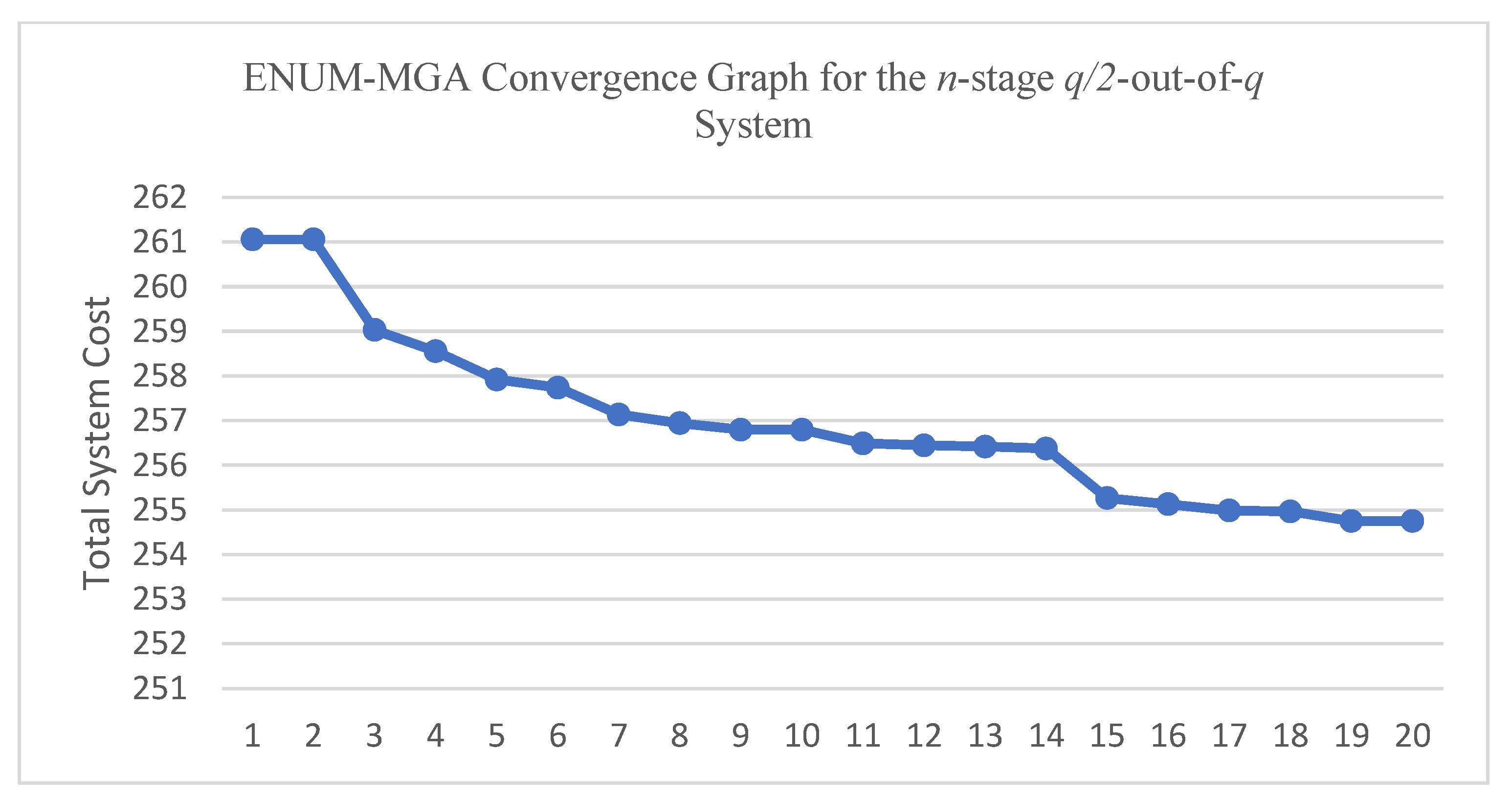
Table 25 demonstrates that for the total system costs of 20 simulation runs, the average total system cost equals 256.9299 and the lowest total system cost equals 254.75. The convergence graph in
Figure 13 explicitly indicates that the total system cost can likely be ameliorated and converged for the main
n-stage
q/2-out-of-
q system by applying the proposed ENUM–MGA combined method. Furthermore,
Table 26 demonstrates the optimal system cost, the optimal failure rates, the optimal repair rates, the availability of all subsystems, and the system availability for the principal simulation case for
n-stage
q/2-out-of-
q system.
In
Table 26, the optimal total system cost obtained by the ENUM-MGA combined method for the
n-stage
q/2-out-of-
q system, which is just like the
n-stage standby system and parallel-series system, is also much superior to the optimal total system cost obtained by the modified genetic algorithm for the
n-stage single component series system in
Table 6. Furthermore, other simulation results produced by the TS–MGA, SA–MGA, NESA–MGA, and MRAH–MGA combined methods for the
n-stage
q/2-out-of-
q system also prove that the proposed availability optimization decision support design system can apply the component redundancy design of the
n-stage
q/2-out-of-
q system to reduce cost and meet the certain level of the system availability requirement compared to the
n-stage single component series system.
Table 27.
The total system costs of 20 simulation runs obtained by TA–MGA for the n-stage q/2-out-of-q system.
Table 27.
The total system costs of 20 simulation runs obtained by TA–MGA for the n-stage q/2-out-of-q system.
| cr-rate = 0.95 mu-rate = 0.5 GApopulation = 200 GAloop = 200 |
|---|
| Total System Cost (TabuLoop) (CPU Time) |
|---|
| 262.3425(50)(3575.53) | 262.2905(50)(3563.52) | 262.2645(50)(3557.276) | 262.0538(50)(3605.8) |
| 262.0088(50)(3561.249) | 261.7917(50)(3634.4527) | 262.2589(100)(7246.5046) | 260.9296(100)(7143.268) |
| 260.7991(100)(7183.86) | 260.74(100)(7156.376) | 260.34(100)(7161.29) | 259.68(150)(10,747.22) |
| 256.96(150)(10,650.82) | 255.3389(150)(10,727.65) | 255.7538(200)(14,803) | 254.8258(200)(14,318.947) |
| 254.4347(200)(14,404.277) | 254.8747(250)(18,055.384) | 254.8549(250)(17,686.767) | 254.0007*(250)(17,993.076) |
| Lowest Total System Cost (TabuLoop)(CPUTime) 254.0007*(250)(17,993.076) |
| Avg. Total System Cost (TabuLoop) (Avg. CPUTime) |
| 262.1253(50)(3582.97) | 261.01(100)(7178.26) | 257.327(150)(10,708.56) | 255.0048(200)(14,508.74) |
| 254.5768(250)(17,911.74) | | | |
By applying the TA–MGA combined method for the principal
n-stage
q/2-out-of-
q system,
Table 27 above shows 20 selected simulated outcomes of the total system costs by assuming TabuLoop equal to 50 with an average CPU running time of 3582.97 s until 250 with an average CPU running time of 17,911.74 s, and it further converges the average total system cost of 262.1253 to 254.5768 and the total system cost of 262.3425 to the lowest 254.0007. Since the average total system cost of 255.0048 with 200 Tabu loops is just a little higher than 254.5768 with 250 Tabu loops, the simulation process stops running at 250 Tabu loops and finally achieves the lowest converged result of 254.0007. In addition,
Figure 14 illustrates how the total system cost has improved and finally converged for the
n-stage
q/2-out-of-
q system by conducting the proposed TA–MGA combined methods.
Additionally, for the above-mentioned lowest converged total system cost of 254.0007, which is obtained at 250 Tabu loops,
Table 28 displays the optimal system cost related to the optimal failure rates, the repair rates, the availability of all subsystems, and the system availability, as follows:
Table 28.
Optimal Solutions obtained by TA–MGA for the n-stage q/2-out-of-q system.
Table 28.
Optimal Solutions obtained by TA–MGA for the n-stage q/2-out-of-q system.
| TabuLoop = 250 cr-rate = 0.95 mu-rate = 0.5 GApopulation = 200 GAloop = 200 |
|---|
| Decision Variables | Subsystem(i) |
|---|
| | 1 | 2 | 3 | 4 | 5 |
|---|
| 2 | 2 | 4 | 2 | 2 |
| (10−3) | 0.2417 | 0.2132 | 0.1613 | 0.4915 | 0.2629 |
| 0.0018 | 0.0014 | 0.0008 | 0.0022 | 0.0015 |
| 0.9864 | 0.9830 | 0.9810 | 0.9667 | 0.9788 |
| Optimal Total System Cost 254.0007 |
| 0.9000 |
Table 29.
The total system costs of 20 simulation runs obtained by SA–MGA for the n-stage q/2-out-of-q system.
Table 29.
The total system costs of 20 simulation runs obtained by SA–MGA for the n-stage q/2-out-of-q system.
| cr-rate = 0.95 mu-rate = 0.5 GApopulation = 200 GAloop = 200 |
|---|
| Total System Cost (SAloop) (CPU Time) |
|---|
| 283.9753(25)(4042.73) | 283.563(25)(4044.1266) | 262.1185(25)(4047.668) | 261.4488(25)(3961.58) |
| 260.0856(25)(3999.2586) | 257.8223(25)(3954.55) | 257.4265(25)(3968.1949) | 261.1689(50)(8044.036) |
| 257.6876(50)(7999.579) | 256.4644(50)(7875.32) | 254.2033(50)(7946.35) | 253.2374(50)(7989.318) |
| 253.0851(50)(8079.2985) | 251.9111(50)(8077.339) | 251.0012(100)(16,361.8) | 247.9969(100)(16,218.2) |
| 247.0783(100)(16,154.4) | 245.7722(100)(15,967.8) | 243.5175(150)(23,846.4) | 242.8014*(150)(24,025.1) |
| Lowest Total System Cost (SAloop)(CPUTime) 242.8014*(150)(24,025.1) |
| Avg. Total System Cost (SAloop)(CPUTime) |
| 266.6342857(25)(4002.6) | 255.3939714(50)(8001.6) | 247.96215(100)(16,175.5) | 243.15943(150)(23,935.8) |
By applying the SA–MGA combined method to continue the simulated numerical cases for the
n-stage
q/2-out-of-
q system,
Table 29 displays 20 picked simulated outcomes of the total system costs by presuming SAloop equal to 25 with an average CPU running time of 4002.587657 s until 150 with an average CPU running time of 23,935.75 s, and it further converges the average total system cost of 266.6342857 to 243.15943 and the total system cost of 283.9753 to the lowest 242.8014. As the average total system cost of 243.15943 with 150 SA loops is just a little lower than 247.96215 with 100 SA loops, the simulation process ceases at 150 SA loops and converges to the lowest result of 242.8014. Consequently, the convergence graph in
Figure 15 also demonstrates the trend that the total system cost has improved and eventually converged for the principle
n-stage
q/2-out-of-
q system by conducting the proposed SA–MGA combined method.
In addition, for the above lowest converged result of 242.8014, which is obtained at 150 SA loops,
Table 30 shows the optimal system cost related to the optimal failure rates, the optimal repair rates, the availability of all subsystems, and the system availability, as follows:
Table 30.
Optimal Solutions obtained by SA–MGA for the for the n-stage q/2-out-of-q system.
Table 30.
Optimal Solutions obtained by SA–MGA for the for the n-stage q/2-out-of-q system.
| SAloop = 150 cr-rate = 0.95 mu-rate = 0.5 GApopulation = 200 GAloop = 200 |
|---|
| Decision Variables | Subsystem(i) |
|---|
| | 1 | 2 | 3 | 4 | 5 |
|---|
| 2 | 2 | 2 | 2 | 2 |
| (10−3) | 0.2225 | 0.2136 | 0.1470 | 0.5036 | 0.2538 |
| 0.0021 | 0.0014 | 0.0009 | 0.0023 | 0.0014 |
| 0.9904 | 0.9814 | 0.9818 | 0.9672 | 0.9750 |
| Optimal Total System Cost 242.8014 |
| 0.9000 |
Conducting the NESA–MGA combined method to simulate numerical cases for the
n-stage
q/2-out-of-
q system,
Table 31 demonstrates 20 incited simulated consequences of the total system costs by supposing NESAloop equal to 50, which average CPU running time is 1791.623921 s until 150, which average CPU running time is 5351.647619 s, and it further converges the average total system cost of 246.7436125 to 239.555425 and the total system cost of 267.1363 to the lowest 238.6284. As the average total system cost of 239.555425 with 150 NESA loops is pretty close to 239.7594875 with 100 SA loops, the simulation process halts at 150 NESA loops and converges to the lowest outcome of 238.6284.
Table 31.
The total system costs of 20 simulation runs obtained by NESA–MGA for the n-stage q/2 out-of-q system.
Table 31.
The total system costs of 20 simulation runs obtained by NESA–MGA for the n-stage q/2 out-of-q system.
| cr-rate = 0.95 mu-rate = 0.5 GApopulation = 200 GAloop = 200 |
|---|
| Total System Cost (NESAloop) (CPU Time) |
|---|
| 267.1363(50)(1815.2488) | 266.8671(50)(1847.3193) | 240.2965(50)(1748.9829) | 240.2547(50)(1761.1064) |
| 240.0845(50)(1815.1721) | 240.083(50)(1799.07156) | 239.7278(50)(1735.1919) | 239.499(50)(1810.89833) |
| 240.3252(100)(3765.378) | 239.8942(100)(1716.0388) | 239.8309(100)(3499.851) | 239.755(100)(3623.509) |
| 239.7221(100)(3639.3678) | 239.7076(100)(3751.0742) | 239.5324(100)(3512.8106) | 239.3085(100)(3507.3925) |
| 240.099(150)(5112.6764) | 239.9187(150)(5415.5617) | 239.5756(150)(5408.593) | 238.6284*(150)(5469.7597) |
| Lowest Total System Cost (NESAloop)(CPUTime) 238.6284*(150)(5469.7597) |
| Avg. Total System Cost (NESAloop)(CPUTime) |
| 246.7436125(50)(1791.623921) | 239.7594875(100)(3376.927721) | 239.555425(150)(5351.647619) | |
Therefore, the convergence graph in
Figure 16 clearly displays the trend that the total system cost will ameliorate and finally converge for the
n-stage
q/2-out-of-
q system by implementing the proposed NESA–MGA combined method.
Additionally, for the above lowest converged outcome of 238.6284, which is obtained at 150 NESA loops,
Table 32 illustrates the optimal system cost related to the optimal failure rate, the optimal repair rate, the availability of each subsystem, and the system availability, as follows:
Table 32.
Optimal Solutions obtained by NESA–MGA for the for the n-stage q/2-out-of-q system.
Table 32.
Optimal Solutions obtained by NESA–MGA for the for the n-stage q/2-out-of-q system.
| SAloop = 150 cr-rate = 0.95 mu-rate = 0.5 GApopulation = 200 GAloop = 200 |
|---|
| Decision Variables | Subsystem(i) |
|---|
| | 1 | 2 | 3 | 4 | 5 |
|---|
| 2 | 2 | 2 | 2 | 2 |
| (10−3) | 0.2500 | 0.2303 | 0.1509 | 0.4489 | 0.2487 |
| 0.0014 | 0.0014 | 0.0010 | 0.0026 | 0.0015 |
| 0.9760 | 0.9801 | 0.9822 | 0.9776 | 0.9799 |
| Optimal Total System Cost 238.6284 |
| 0.9000 |
Table 33 and
Table 34 display the simulation consequences obtained by the MRAH-MGA combined method for the
n-stage
q/2-out-of-
q system, showing the total system costs of 20 simulation runs, the related average total system cost of 239.999455, and the lowest total system cost equal to 226.8125, which is superior to all other combined methods and has an extremely low average CPU running time of around 262.7216 s.
Table 33.
The total system costs of 20 simulation runs obtained by MRAH–MGA for the n-stage q/2- out-of-q system.
Table 33.
The total system costs of 20 simulation runs obtained by MRAH–MGA for the n-stage q/2- out-of-q system.
| cr-rate = 0.95 mu-rate = 0.5 GApopulation = 200 GAloop = 200 |
|---|
| Total System Cost (CPU Time) |
|---|
| 243.3626(266.64) | 241.8375(261.93) | 241.6838(258.7) | 241.6701(256.99) | 241.43(265.25) | 240.9255(263.05) |
| 240.9255(256.75) | 240.9154(270.45) | 240.8245(255.27) | 240.7902(260.678) | 240.6668(257) | 240.2744(272.2) |
| 239.8724(270.69) | 239.872(283.1) | 239.872(255.66) | 239.6613(262.1) | 239.5804(255.9) | 239.506(263.87) |
| 239.5061(258.029) | 226.8125*(260.12) | | | | |
| Lowest Total System Cost (CPU Time)
226.8125*(260.12) |
| Avg. Total System Cost (Avg. CPU Time)
239.999455(262.7216) |
Table 34.
Optimal Solutions obtained by MRAH–MGA for the n-stage q/2-out-of-q system.
Table 34.
Optimal Solutions obtained by MRAH–MGA for the n-stage q/2-out-of-q system.
| Decision Variables | Subsystem(i) |
|---|
| | 1 | 2 | 3 | 4 | 5 |
|---|
| 2 | 2 | 2 | 2 | 2 |
| (10−3) | 0.3184 | 0.2656 | 0.2125 | 0.4842 | 0.3759 |
| 0.0020 | 0.0015 | 0.0009 | 0.0023 | 0.0018 |
| 0.9922 | 0.9626 | 0.9886 | 0.9635 | 0.9932 |
| Optimal Total System Cost 226.8125 |
| System Availability 0.903544 |
Additionally,
Figure 17 demonstrates that the total system cost is improved and converged for the main
n-stage
q/2-out-of-
q system by executing the proposed MRAH–MGA combined method.
4.5. The Simulation Case for n-Stage Mixed System
In the previous four sections, the proposed availability optimization decision support design system has designed four individual systems, including an
n-stage single component system,
n-stage standby system, parallel-series system, and
n-stage
q/2-out-of-
q system, which all have subsystems assumed to be the same configuration. Yet, in the real world, the actual system is generally complicated and comprises various subsystems with different configurations. Next, the availability optimization decision support design system aims to design the
n-stage mixed systems with different combinations of subsystems, including a standby, parallel, and
q/2-out-of-
q connected in series configuration. This study will further conduct the simulation cases by adopting the ENUM-MGA, TA–MGA, SA–MGA, NESA–MGA, and MRAH–MGA combined methods for one specific
n-stage mixed system, which comprises two parallel subsystems, two standby subsystems, and one
q/2-out-of-
q subsystem.
Table 35 and
Table 36 show the simulation results of the ENUM–MGA combined method.
Table 37 and
Table 38 display the simulation outcomes produced by the TA–MGA combined method.
Table 39 and
Table 40 demonstrate the simulation results generated by the SA–MGA combined method.
Table 41 and
Table 42 show the simulation outcomes created by the NESA–MGA combined method.
Table 43 and
Table 44 display the simulation outcomes resulting from the MRAH–MGA combined method.
Regarding the simulation cases of the
n-stage mixed system, the numerical results obtained by the ENUM-MGA combined method is illustrated in the following
Table 34 and
Table 36 and
Figure 18.
Table 35 shows the total system costs of 20 simulation runs, in which the average total system cost equals 228.43785 and the lowest total system cost equals 227.164. The convergence graph in
Figure 18 denotes that the total system cost has improves and converged for the
n-stage mixed system by enforcing the proposed ENUM–MGA combined method. Furthermore,
Table 35 demonstrates the optimal system cost, the optimal failure rates, the optimal repair rates, the availability of all subsystem, and the system availability for the principal simulation case of the
n-stage mixed system.
By adopting the TA–MGA combined method for the
n-stage mixed system, 20 picked simulated results of the total system costs are displayed in the following
Table 37 by setting TabuLoop equal to 50 with an average CPU running time of 2207.1796 s until 250 with an average CPU running time of 11,108.103 s, and they are further converged from the average total system cost of 228.8267 to 221.294 and from the total system cost of 229.1124 to the lowest 221.1764. Since the average total system cost of 221.9263083 with 200 Tabu loops is just a little higher than 221.294 with 250 Tabu loops, the simulation process stops running at 250 Tabu loops and finally achieves the lowest converged result of 221.1764.
Table 37.
The total system costs of 20 simulation runs acquired by TA–MGA combined method for the n-stage mixed system.
Table 37.
The total system costs of 20 simulation runs acquired by TA–MGA combined method for the n-stage mixed system.
| cr-rate = 0.95 mu-rate = 0.5 GApopulation = 200 GAloop = 200 |
|---|
| Total System Cost (TabuLoop) (CPU Time) |
|---|
| 229.1124(50)(2227.49) | 228.541(50)(2186.86) | 225.9619(100)(4345.43) | 225.0738(100)(4470.18) |
| 223.2599(150)(6641.27) | 222.8208(150)(6655.76) | 222.5571(200)(9621.79) | 222.1876(200)(9335.25) |
| 221.9989(200)(9412.08) | 221.9579(200)(9410.79) | 221.9419(200)(9498.078) | 221.8878(200)(9814.1) |
| 221.8746(200)(8811.95) | 221.8395(200)(9169.73) | 221.8395(200)(8834.7) | 221.7808(200)(8776.96) |
| 221.6745(200)(10,261.2) | 221.5756(200)(8838.7) | 221.4116(250)(11,185) | 221.1764*(250)(11,031.066) |
| Lowest Total System Cost(TabuLoop)(CPUTime) 221.1764*(250)(11,031.066) |
| Avg. Total System Cost (TabuLoop)(CPUTime) |
| 228.8267(50)(2207.1796) | 225.51785(100)(4407.8031) | 223.04035(150)(6648.5153) | 221.9263083(200)(9315.444) |
| 221.294(250)(11,108.103) | | | |
Moreover, the convergence graph in
Figure 19 illustrates how the total system cost has been reformed and at last converged for the
n-stage mixed system by implementing the proposed TA–MGA combined method.
Regarding the above lowest optimal total system cost of 221.1764, which is converged at 250 TA loops,
Table 38 delineates the detailed information, including the optimal failure rates, the optimal repair rates, the availability of all subsystems, and the system availability.
Table 38.
Optimal Solutions obtained by TA–MGA combined method for the n-stage mixed system.
Table 38.
Optimal Solutions obtained by TA–MGA combined method for the n-stage mixed system.
| cr-rate = 0.95 mu-rate = 0.5 GApopulation = 200 GAloop = 200 |
|---|
| Decision Variables | Subsystem(i) |
|---|
| | 1 | 2 | 3 | 4 | 5 |
|---|
| 3 | 3 | 2 | 3 | 2 |
| (10−3) | 0.3511 | 0.2778 | 0.1402 | 0.6599 | 0.2538 |
| 0.0010 | 0.0010 | 0.0009 | 0.0015 | 0.0014 |
| 0.9838 | 0.9846 | 0.9816 | 0.9716 | 0.9743 |
| Optimal Total System Cost 221.1764 |
| 0.9000 |
By employing the SA–MGA combined method to execute the simulated numerical examples for the
n-stage mixed system, the following
Table 39 displays 21 picked simulated results of the total system costs by supposing SAloop equal to 50 with an average CPU time of 4050.163 s until 150 with an average CPU time of 14,840.777 s, and it further converges the average total system cost of 228.4432 to 222.2532 and the total system cost of 229.2389 to the lowest 222.2532. For the case when the average total system cost of 222.2532 with 150 SA loops is lower than 222.2608 with 200 SA loops, the simulation process ceases at 150 SA loops and converges to the lowest total system cost of 222.2532.
Table 39.
The total system costs of 21 simulation runs obtained by SA–MGA for the n-stage mixed system.
Table 39.
The total system costs of 21 simulation runs obtained by SA–MGA for the n-stage mixed system.
| cr-rate = 0.95 mu-rate = 0.5 GApopulation = 200 GAloop = 200 |
|---|
| Total System Cost (SAloop) (CPU Time) |
|---|
| 229.2389(50)(4970.83) | 228.4881(50)(2227.22) | 227.6027(50)(4952.435) | 225.5595(100)(9425.54) |
| 225.5595(100)(10,604.14) | 224.8517(100)(9812.857) | 224.7499(100)(9550.08) | 224.4633(100)(9920.997) |
| 224.4258(100)(9953.296) | 224.3913(100)(9775.858) | 224.0892(100)(9659.037) | 224.0892(100)(10,342.6) |
| 224.0509(100)(9603.48) | 224.0509(100)(10,283.213) | 224.0485(100)(9558.37) | 224.0485(100)(9420.227) |
| 223.698(100)(9663.32) | 223.698(100)(16,025.8) | 222.2665(150)(14,807.37) | 222.2532*(150)(14,874.18) |
| 222.2608(200)(20,724.566) | | | |
| Lowest Total System Cost (SAloop)(CPUTime) 222.2532*(150)(14,874.18) |
| Avg. Total System Cost (SAloop)(CPUTime) |
| 228.4432(50)(4050.163) | 224.3849467(100)(224.384947) | 222.25985(150)(14,840.777) | |
Consequently, the convergence graph in
Figure 20 demonstrates the trend that the total system cost has improved and in the end converged for the
n-stage mixed system by utilizing the proposed SA–MGA combined method.
In addition, for the above lowest converged result of 222.2532, which is acquired at 150 SA loops,
Table 40 describes the detailed information, including the optimal system cost, the optimal failure rates, the optimal repair rates, the availability of all subsystems, and the system availability, as follows:
Table 40.
Optimal Solutions obtained by SA–MGA for the for the n-stage mixed system.
Table 40.
Optimal Solutions obtained by SA–MGA for the for the n-stage mixed system.
| SAloop =150 cr-rate = 0.95 mu-rate = 0.5 GApopulation = 200 GAloop = 200 |
|---|
| Decision Variables | Subsystem(i) |
|---|
| | 1 | 2 | 3 | 4 | 5 |
|---|
| 3 | 3 | 2 | 3 | 2 |
| (10−3) | 0.3409 | 0.2825 | 0.1563 | 0.6524 | 0.2629 |
| 0.0011 | 0.0010 | 0.0010 | 0.0014 | 0.0015 |
| 0.9872 | 0.9839 | 0.9823 | 0.9668 | 0.9756 |
| Optimal Total System Cost 222.2532 |
| 0.9000 |
Employing the NESA–MGA combined method to simulate numerical cases of the
n-stage mixed system,
Table 41 illustrates 20 chosen simulated outcomes of the total system costs by assuming NESAloop equal to 50, which an average CPU running time is 1104.221 s until 200, which an average CPU running time is 4383.1 s, and it further converges the average total system cost of 224.20025 to 221.49795 and the total system cost of 224.841 to the lowest 221.4456. For the reason that the average total system cost of 221.99705 with 150 NESA loops is pretty close to 221.49795 with 200 NESA loops, the simulation process halts at 200 NESA loops and converges to the lowest outcome of 221.4456.
Table 41.
The total system costs of 20 simulation runs obtained by NESA–MGA for the n-stage mixed system.
Table 41.
The total system costs of 20 simulation runs obtained by NESA–MGA for the n-stage mixed system.
| cr-rate = 0.95 mu-rate = 0.5 GApopulation = 200 GAloop = 200 |
|---|
| Total System Cost (NESAloop) (CPU Time) |
|---|
| 224.841(50)(1132.647) | 223.5595(50)(1075.794) | 224.1458(100)(2100.519) | 224.0577(100)(2051.946) |
| 223.2254(100)(2173.69) | 223.2249(100)(2084.81) | 223.1785(100)(2073.37) | 223.1368(100)(1930.83) |
| 223.1191(100)(2039.28) | 223.0354(100)(1963.96) | 222.8479(100)(2072.59) | 222.7554(100)(2108.03) |
| 222.7554(100)(2108.03) | 222.7554(100)(2101.82) | 222.6034(100)(2112.59) | 222.4549(100)(1987.02) |
| 222.4549(100)(2005.96) | 222.5399(150)(3335.04) | 221.4542(150)(3330.326) | 221.5503(200)(4490.57) |
| 221.4456*(200)(4275.63) |
| Lowest Total System Cost (NESAloop)(CPUTime) 221.4456*(200)(4275.63) |
| Avg. Total System Cost (NESAloop)(CPUTime) |
| 224.20025(50)(1104.221) | 223.07111(100)(2057.601) | 221.99705(150)(3332.682) | 221.49795(200)(4383.1) |
Accordingly, the convergence graph in
Figure 21 displays the trend that the total system cost of the
n-stage mixed system can be bettered and eventually converged by utilizing the proposed NESA–MGA combined method.
Regarding the above lowest optimal total system cost of 221.4456, which is obtained at 200 NESA loops, the following
Table 42 delineates the complete information, including the optimal total system cost, the optimal failure rates, the optimal repair rates, the availability for all subsystems, and the system availability.
Table 42.
Optimal Solutions obtained by NESA–MGA for the for the n-stage mixed system.
Table 42.
Optimal Solutions obtained by NESA–MGA for the for the n-stage mixed system.
| SAloop = 150 cr-rate = 0.95 mu-rate = 0.5 GApopulation = 200 GAloop = 200 |
|---|
| Decision Variables | Subsystem(i) |
|---|
| | 1 | 2 | 3 | 4 | 5 |
|---|
| 3 | 3 | 2 | 3 | 2 |
| (10−3) | 0.3670 | 0.2758 | 0.1482 | 0.5969 | 0.2498 |
| 0.0010 | 0.0010 | 0.0011 | 0.0013 | 0.0014 |
| 0.9818 | 0.9839 | 0.9855 | 0.9701 | 0.9746 |
| Optimal Total System Cost 221.4456 |
| 0.9000 |
According to
Table 42, the simulation outcomes acquired by the MRAH-MGA combined method for the
n-stage mixed system are classified into two modes based on the different parameter design for the modified genetic algorithm. Mode 1 applies the originally proposed parameter design for the modified genetic algorithm—which assumes a chromosome crossover rate equal to 0.95, a chromosome mutation rate equal to 0.5, a chromosome population equal to 200, and a genetic generation equal to 200—to obtain the total system costs of 20 simulation runs with the average total system cost of 223.72877 and the lowest total system cost equal to 222.0561. The outcomes acquired from mode 1 are worse than the other combined methods, except for the ENUM-MGA and SA-MGA combined methods. Therefore, mode 2 adopts the other parameter design for the modified genetic algorithm—which assumes a chromosome crossover rate equal to 0.95, a chromosome mutation rate equal to 0.05, a chromosome population equal to 50, and a genetic generation equal to 50—to obtain the total system costs of 20 simulation runs with the average total system cost of 234.300425 and the lowest total system cost equal to 216.977. Comparing the performance between mode 1 and mode 2, the lowest total system cost of mode 2 is apparently lower than that of mode 1, but the average total system cost of mode 2 is higher than that of mode 1. The main reason for this is that the variance of the total system cost acquired from mode 2 of 90.67164485 is much bigger than that of mode 1 at 1.346792558. Therefore, even when the average total system cost of mode 2 is bigger than that of mode 1, there still exists the simulation result, in which the lowest total system cost of mode 2 is significantly lower than that of mode 1 and the other four combined methods, and it has an extremely low CPU running time of around 7.691521 s. The convergence graph in
Figure 22 further displays the trends of the total system costs of the
n-stage mixed system by implementing the proposed mode 1 MRAH–MGA combined method and the mode 2 MRAH–MGA combined method.
Table 43.
The total system costs of 40 simulation runs obtained by MRAH–MGA for the n-stage mixed system.
Table 43.
The total system costs of 40 simulation runs obtained by MRAH–MGA for the n-stage mixed system.
| Mode 1: cr-rate = 0.95 mu-rate = 0.5 GApopulation = 200 GAloop = 200 |
|---|
| Mode 2: cr-rate = 0.95, mu-rate = 0.05, GApopulation = 50, GAloop = 50 |
|---|
| Total System Cost (CPU Time)(Mode) |
|---|
| 225.6124(117.52)(1) | 225.4198(117.01)(1) | 225.0842(116.427)(1) | 225.0159(116.804)(1) | 225.0068(117.214)(1) |
| 224.7567(119.738)(1) | 224.4263(111.36)(1) | 223.9598(112.564)(1) | 223.8361(118.652)(1) | 223.7809(110.09)(1) |
| 223.6381(109.987)(1) | 223.5414(117.902(1) | 223.1572(117.8)(1) | 223.0616(117.35)(1) | 222.9696(115.826)(1) |
| 222.6717(117.809)(1) | 222.4027(112.205)(1) | 222.1095(116.968)(1) | 222.0686(110.17)(1) | 222.0561(114.55)(1) |
| 251.287(7.585734)(2) | 246.9526(7.664593)(2) | 243.9434(7.705879)(2) | 243.6529(7.59)(2) | 242.9158(7.652)(2) |
| 242.087(7.599641)(2) | 240.1311(7.584795)(2) | 239.9994(15.7473)(2) | 234.6201(9.6669)(2) | 232.8847(7.748)(2) |
| 232.8333(7.847)(2) | 232.7708(7.614695)(2) | 232.3982(7.707281)(2) | 229.2715(7.6298)(2) | 228.2998(7.585)(2) |
| 28.2592(7.599764)(2) | 227.8516(8.261175)(2) | 220.0629(7.555221)(2) | 218.8102(7.59)(2) | 216.977(7.692)(2) |
| Lowest Total System Cost(CPU)(mode) 222.0561(114.55)(1) 216.977*(7.691521)(2) |
| Avg. Total System Cost(CPU)(mode) 223.72877*(115.39779)(1) 234.300425(8.1814052)(2) |
| Var. Total System Cost(mode) 1.346792558*(1) 90.67164485(2) |
In light of the lowest converged result of 216.977, which is obtained by mode 2 of the MRAH-MGA combined method,
Table 44 delineates the complete information comprising the optimal component redundancy amounts, the optimal failure rates, the optimal repair rates, the availability for all subsystems, the system availability, and the optimal total system cost, as follows:
Table 44.
Optimal Solutions obtained by mode 2 of MRAH–MGA for the for the n-stage mixed system.
Table 44.
Optimal Solutions obtained by mode 2 of MRAH–MGA for the for the n-stage mixed system.
| cr-rate = 0.95, mu-rate = 0.05, GApopulation = 50, GAloop = 50 |
|---|
| Decision Variables | Subsystem(i) |
|---|
| | 1 | 2 | 3 | 4 | 5 |
|---|
| 3 | 3 | 2 | 3 | 2 |
| (10−3) | 0.3515 | 0.3115 | 0.2880 | 0.5268 | 0.3496 |
| 0.0009 | 0.0010 | 0.0016 | 0.0012 | 0.0017 |
| 0.9805 | 0.9951 | 0.9898 | 0.9594 | 0.9800 |
| Optimal Total System Cost 216.977 |
| 0.90806 |
4.6. The Comparison of Five Proposed System Configurations
According to the results from
Table 3,
Table 4,
Table 5,
Table 6,
Table 7,
Table 8,
Table 9,
Table 10,
Table 11,
Table 12,
Table 13,
Table 14,
Table 15,
Table 16,
Table 17,
Table 18,
Table 19,
Table 20,
Table 21,
Table 22,
Table 23,
Table 24,
Table 25,
Table 26,
Table 27,
Table 28,
Table 29,
Table 30,
Table 31,
Table 32,
Table 33,
Table 34,
Table 35,
Table 36,
Table 37,
Table 38,
Table 39,
Table 40,
Table 41,
Table 42,
Table 43 and
Table 44, the optimal total system cost and CPU running time based on the four proposed system configurations and the five proposed combined methods are further collected and rearranged as the following
Table 45.
According to the results of
Table 45, all optimal total system costs obtained by the ENUM-MGA, TS-MGA, SA-MGA, NESA-MGA, and MRAH-MGA combined methods for the
n-stage standby system, parallel-series system,
n-stage
q/2-out-of-
q system, and
n-stage mixed system are comprehensively much better than the optimal total system cost of 545.489 obtained by the genetic algorithm for the
n-stage single component series system. Therefore, it is demonstrated clearly that the proposed availability optimization decision support design system can easily apply different component redundancy system designs to save a lot of cost and reach the high standard of the system availability requirement compared to the
n-stage single component series system.
Additionally, from the outcomes in
Table 45, all optimal total system costs obtained by the ENUM-MGA, TA-MGA, SA-MGA, NESA-MGA, and MRAH-MGA combined methods for the parallel-series system are apparently lower than those obtained for the
n-stage standby system. Notably, the difference between the standby subsystem and the parallel subsystem is that for the parallel subsystem, all of the components are in operational condition, but for the standby subsystem, only one component is in operational condition and all of the other components are in standby condition. Since this study assumes the same deteriorating probability for operating components and for standby components, the parallel subsystem can clearly meet the same level of availability requirement with less cost compared to the standby subsystem. This is why in this study, the optimal total system cost for the parallel-series system is lower than the
n-stage standby system. However, in the real world, the deteriorating situation of the standby component should be better than the operating component. This could lead to the cost saving of the standby subsystem to cover the original advantage of the parallel subsystem in order to easily reach high-level availability.
Moreover,
Table 45 also shows that all of the optimal total system costs obtained by the ENUM-MGA, TA-MGA, SA-MGA, NESA-MGA, and MRAH-MGA combined methods for the
n-stage
q/2-out-of-
q system are higher than those obtained for the
n-stage standby system and parallel-series system, which can be verified easily from the aspect of system configuration structure and system availability theory.
Finally, the proposed
n-stage mixed system in this study comprises two parallel subsystems, two standby subsystems, and one
q/2-out-of-
q subsystem. Therefore,
Table 45 clearly displays that all of the optimal total system costs acquired by the ENUM-MGA, TA-MGA, SA-MGA, NESA-MGA, and MRAH-MGA combined methods for this
n-stage mixed system are higher than the parallel-series system, but lower than the
n-stage standby system and the
n-stage
q/2-out-of-
q system.
4.7. The Performance Comparison of Five Proposed Combined Methods
Based on the outcomes from
Table 4,
Table 5,
Table 6,
Table 7,
Table 8,
Table 9,
Table 10,
Table 11,
Table 12,
Table 13,
Table 14,
Table 15,
Table 16,
Table 17,
Table 18,
Table 19,
Table 20,
Table 21,
Table 22,
Table 23,
Table 24,
Table 25,
Table 26,
Table 27,
Table 28,
Table 29,
Table 30,
Table 31,
Table 32,
Table 33,
Table 34,
Table 35,
Table 36,
Table 37,
Table 38,
Table 39,
Table 40,
Table 41,
Table 42,
Table 43,
Table 44 and
Table 45, the performance comparisons of the five proposed combined methods for the four proposed system configurations are illustrated and analyzed completely as follows.
Comparing the performance of the five combined methods for the n-stage standby system, the optimal system cost is 243.2092 for the ENUM-MGA combined method, 236.831 for the TS-MGA combined method, 236.463 for the SA-MGA combined method, 237.27 for the NESA-MGA combined method, and 226.45 for the MRAH -MGA combined method. The performance ranking regarding the criteria of the optimal total system cost has the sequence MRAH-MGA, SA-MGA, TS-MGA, NESA-MGA, ENUM-MGA. Moreover, the CPU running time is 2697.3 s for the ENUM-MGA combined method, 7641 s for the TA–MGA combined method, 21,232.9 s for the SA–MGA combined method, 9441.45 s for the NESA–MGA combined method, and 5.31 s for the MRAH–MGA combined method. Therefore, the performance ranking regarding the criteria of CPU running time has the order MRAH-MGA, ENUM-MGA, TA-MGA, NESA-MGA, SA-MGA. Consequently, for the n-stage standby system, the optimal total system cost obtained by conducting the MRAH-MGA combined method is superior to all of the other combined methods, and it also has an extreme and lowest CPU running time of around 5.31 s.
To compare the performance of the five combined methods for the parallel-series system, the optimal total system cost is 220.278 for the ENUM-MGA combined method, 214.62 for the TS-MGA combined method, 214.7569 for the SA-MGA combined method, 214.9928 for the NESA-MGA combined method, and 208.9659 for the MRAH-MGA combined method. The performance ranking regarding the criteria of the optimal total system cost is ranked as the sequence MRAH-MGA, TS-MGA, SA-MGA, NESA-MGA, ENUM-MGA. Moreover, the CPU running time is 2696.55 s for the ENUM-MGA combined method, 9361 s for the TS-MGA combined method, 8182.35 s for the SA–MGA combined method, 12,864.215 s for the NESA-MGA combined method, and 98.64 s for the MRAH–MGA combined method. Therefore, the performance ranking regarding the criteria of CPU running time has the order MRAH-MGA, ENUM-MGA, SA-MGA, TS-MGA, NESA-MGA. Consequently, for the parallel-series system, the optimal total system cost obtained by conducting the MAHA-GA combined method is superior to all of the other combined methods, and it also has an extreme and lowest CPU running time of around 98.64 s.
Concerning the performance of the five different combined methods for the n-stage q/2-out-of-q system, the optimal system cost is 254.75 for the ENUM-MGA combined method, 254.0007 for the TA–MGA combined method, 242.8014 for the SA–MGA combined method, 238.6284 for the NESA–MGA combined method, and 226.8125 for the MRAH–MGA combined method. As a result, the performance ranking concerning the criteria of the optimal total system cost has the order MRAH-MGA, NESA-MGA, SA-MGA, TS-MGA, ENUM-MGA. Additionally, the CPU running time is about 4763.557856 s for the ENUM-MGA combined method, 17,993.076 s for the TA–MGA combined method, 24,025.088 s for the SA–MGA combined method, 5469.7597 s for the NESA–MGA combined method, and 260.12 s for the MRAH-MGA combined method. Therefore, the performance ranking for the criteria of CPU running time has the sequence MRAH-MGA, ENUM-MGA, NESA-MGA, TA-MGA, SA-MGA. Accordingly, with regard to the n-stage q/2-out-of-q system, the optimal total system cost obtained by conducting the MRAH-MGA combined method is evidently better than all of the other combined methods, and it also has the lowest CPU running time of 98.64 s.
Regarding the performance of the five different combined methods for the n-stage mixed system, the optimal system cost is 227.164 for the ENUM-MGA combined method, 221.1764 for the TS-MGA combined method, 222.2532 for the SA-MGA combined method, 221.4456 for the NESA-MGA combined method, and 216.977 for mode 1 of the MRAH-MGA combined method. Therefore, the performance ranking concerning the criteria of the optimal total system cost has the ranked mode 1 sequence MRAH-MGA, TS-MGA, NESA-MGA, SA-MGA, ENUM-MGA. In addition, the CPU running time is about 3072.13 s for the ENUM-MGA combined method, 11,031.066 s for the TS-MGA combined method, 14,874.18 s for the SA-MGA combined method, 4275.63 s for the NESA-MGA combined method, and 7.691521 s for the MRAH-MGA combined method. Therefore, the performance ranking for the criteria of CPU running time has the sequence MRAH-MGA, ENUM-MGA, NESA-MGA, TS-MGA, SA-MGA. Accordingly, regarding the n-stage mixed system, the optimal total system cost obtained by conducting mode 1 of the MRAH-MGA combined method is significantly better than all of the other combined methods, it also has the lowest CPU running time of 7.691521 s.
Concluding the above comparison results, the following
Table 46 and
Table 47 demonstrate the detailed performance ranking and the relative comparison indices of the optimal total system cost and CPU running time for the five proposed combined methods based on the four proposed system configurations.
Summarizing the performances of the optimal total system cost in
Table 46, the MRAH-MGA combined method ranks in the top spot for all proposed four system configurations; the TA-MGA combined method ranks in the second spot for two proposed system configurations, the third spot for one proposed system configuration, and the fourth spot for one proposed system configuration; the SA-MGA combined method ranks in the second spot for one proposed system configuration, the third spot for two system configurations, the second spot for one proposed system configuration, the third spot for two proposed system configurations, and the fourth spot for one system configuration; the NESA-MGA combined method ranks in the second spot for one system configuration, the third spot for one system configuration, and the fourth spot for two system configurations; and the ENUM-MGA combined method ranks last for all system configurations. Furthermore, from the view of the total performance ranking of the optimal system cost, the MRAH–MGA combined method (4) is in the first spot, the TS–GA combined method (11) is in the second spot, the SA-MGA combined method (12) is in the third spot, the NESA-MGA combined method (13) is in the fourth spot, and the ENUM-MGA combined method (20) is in the last spot. Therefore, it is evident that the performance of the optimal system cost for the MRAH–MGA combined method significantly surpasses the other four combined methods.
In addition, regarding to the performances of the CPU running time in
Table 46, the MRAH-MGA combined method ranks in first place for all system configurations; the ENUM-MGA combined method ranks in second place for all system configurations; the NESA-MGA combined method ranks in third place for two system configurations, second place for one system configuration, and fourth place for one system configuration; the TS-MGA combined method ranks in third place for one system configuration and fourth place for three system configurations; and the SA-MGA combined method ranks in third place for one system configuration and the last place for three system configurations. Moreover, in terms of the total performance ranking of CPU running time, the MRAH–MGA combined method (4) is in first place, the ENUM–MGA combined method (8) is in second place, the TS-MGA combined method (15) and NESA-MGA combined method (13) are both in third place, and the SA-MGA combined method (18) is in last place. Therefore, it is evident that the performance of the CPU running time for the MRAH-MGA combined method is largely superior to the other four combined methods.
The relative compared indices for the optimal total system cost and CPU running time is determined as the ratio 1 for the lowest outcome, and the ratios for the other four combined methods are their values divided by the value of the lowest outcome.
Table 47 expresses the values for all five proposed combined methods. In
Table 47, the average relative compared index for the optimal total system cost acquired by MRAH-MGA is 1, NESA-MGA is 1.0373, SA-MGA is 1.0417, ENUM-MGA is 1.0469, and TS-MGA is 1.053. The performance of the optimal total system cost from the MRAH-MGA combined method is almost 3.73% superior to NESA-MGA, 4.17% superior to SA-MGA, and 4.69% superior to ENUM-MGA. Furthermore, the average relative compared index for the CPU running time from the MRAH–MGA combined method is 1, the ENUM-MGA combined method is 238.276, the NESA-MGA combined method is 496.3765, the TA-MGA combined method is 759.387, and the SA-MGA combined method is 1527.0562. The performance of CPU running time from the MRAH-MGA combined method is approximately 237 times superior to the ENUM-MGA combined method, 497 times superior to the NESA-MGA combined method, 758 times superior to the TA–MGA combined method, and 1526 times superior to the SA–MGA combined method. Therefore, it can be concluded that the performance of the MRAH-MGA combined method in acquiring the optimal system cost is not only superior to the other four combined methods, but the performance of the MRAH-MGA combined method in CPU running time is also superior compared to the other four proposed combined methods. The main reason for this is that system configuration constraints restrict the number of redundancy components in cases of a smaller ceiling, thus the proposed well-designed heuristic approach of MRAH has no difficulty finding the optimal redundant component amount to reach the optimal total system cost, even with much less CPU running time compared to TS, SA, NESA, and ENUM.


