Abstract
In this paper, we present a finite-time synchronization (FTS) for quantized Markovian-jump time-varying delayed neural networks (QMJTDNNs) via event-triggered control. The QMJTDNNs take into account the effects of quantization on the system dynamics and utilize a combination of FTS and event-triggered communication to mitigate the effects of communication delays, quantization error, and efficient synchronization. We analyze the FTS and convergence properties of the proposed method and provide simulation results to demonstrate its effectiveness in synchronizing a network of QMJTDNNs. We introduce a new method to achieve the FTS of a system that has input constraints. The method involves the development of the Lyapunov–Krasovskii functional approach (LKF), novel integral inequality techniques, and some sufficient conditions, all of which are expressed as linear matrix inequalities (LMIs). Furthermore, the study presents the design of an event-triggered controller gain for a larger sampling interval. The effectiveness of the proposed method is demonstrated through numerical examples.
Keywords:
Lyapunov–Krasovskii functional; event-triggered control; neural networks; synchronization; finite-time stability MSC:
37C75; 60J25; 93D40; 34D20
1. Introduction
Because of their superiority in managing data and learning algorithms, neural networks (NNs) have piqued the interest of numerous academics in many domains over the past several decades. As a result, NNs have extensive applications in a variety of fields, including image processing, financial markets, combinatorial optimization, and fixed-point calculations [1,2,3]. Meanwhile, Markovian-jump time-varying delayed neural networks (MJTDNNs) are a type of neural network that incorporates a Markovian-jump process into their dynamics. This allows the network to switch between different modes of operation, depending on the system’s present condition [4,5,6]. The Markovian-jump process is a mathematical model that describes how the system state changes over time, with different modes or states having different dynamics. The transmission of axonal signals usually creates delays in all neural networks, causing unexpected changing network phenomena, such as oscillation and instability [1,2,3,4].
In recent years, research on neural networks has been increasingly preoccupied with the concept of finite-time (FT) stability. For a very long time, one of the most important areas of research has concerned the stability of dynamic systems. The Lyapunov stability methodology has been extensively employed by academics for the purpose of assessing system stability [7,8,9,10]. Yet, throughout the course of the past several years, academics have additionally been focusing more of their attention on the performance needs of dynamic systems in finite time. Since Dorato and Weiss first presented the idea of FT stability in 1961 and 1967, respectively [11,12], numerous facets of FT stability, such as boundedness, stability, stabilization, and synchronization, have also been extensively researched, including both linear as well as nonlinear systems [8,9,13]. The issue of achieving FT stability or synchronization in quantized Markovian-jump time-varying delayed neural networks (QMJTDNNs) is a crucial and difficult field of research. Markovian-jump neural networks have the ability to undergo sudden changes in their dynamics or structure due to external factors or disturbances. Quantization introduces additional complexity, as it causes errors that can affect the system’s stability and synchronization. The interaction between random jumps, quantization errors, and control laws presents a significant challenge, and developing effective control laws for these systems is crucial for their performance in areas such as robotics, communication, and signal processing. However, there is a dearth of literature on the topic of FT stability or synchronization for QMJTDNNs [14,15,16,17].
Synchronization is an important topic that has gained a lot of attention due to its wide range of applications in secure communication [18], image encryption [19], and information science [16]. Drive–response synchronization is a popular area of research, where the goal is to synchronize a drive model with a response model using appropriate controllers. Several control methods have been developed, such as intermittent control [20], impulsive control [21], and sliding-mode control [22]. However, constant control gains are often designed to satisfy the synchronization condition, which can be far greater than necessary, making it uneconomical. Adaptive control can address this issue by designing dynamic control gains that adjust automatically based on the system’s state. In neuroscience, synchronization is a critical mechanism of neural information transmission and processing and is a typical form of neuronal cluster firing activity, which promotes normal brain functions such as cognition, emotion, and behavior. NNs are made up of many nodes that are connected to each other and have the following key features: (1) NNs contain a large number of interconnected neurons, (2) they have diverse junctions where the weights of connections can vary and point in different directions, and (3) the activation function of neurons is nonlinear [23]. Since NNs have such complicated properties, they may be utilized in a wide variety of contexts, with the specific applications being determined by the dynamic properties of the linked networks, notably in terms of synchronization [17]. At present, the synchronization of QMJTDNNs is still a challenging research field, and the related research is scarce [24,25]. Furthermore, the synchronization of NNs has been recognized as a key research topic due to the complex and dynamic behavior of coupled nodes. This dynamic behavior allows for a broad variety of applications, including the detection of shock patterns in physical systems and secure communication using synchronization-based cryptography, amongst others [15,26], and so on.
Quantization is an essential aspect in the process of networked control systems, as it reduces the communication burden and reduces the effect of noise and quantization errors [27,28,29,30]. However, the presence of quantization may also result in a decline in the performance of the system. In addition, the presence of time-varying delays in the networks can lead to additional difficulties in achieving synchronization. To address these challenges, we propose a system based on the combination of quantized control and event-triggered (ET) strategies, which effectively reduces the communication burden and improves the system’s performance [31,32,33]. The ET scheme only updates the control inputs when the system’s state deviates from a predefined neighborhood, thus reducing the number of transmissions and improving the system’s efficiency [34,35,36,37,38]. Actuator saturation is a typical event in the field of control systems where the actuator, which is responsible for controlling the system’s behavior, reaches its maximum or minimum limit. ET control can also be used to mitigate actuator saturation by reducing the frequency of updates to the actuator. This is because ET control only updates the actuator when a triggering event occurs, rather than continuously, which can reduce the likelihood of the actuator becoming saturated. However, ET control can also introduce new challenges, such as determining the appropriate triggering threshold and ensuring that the triggering events occur often enough to maintain the system’s performance. An investigation of ET synchronization for time-delayed recurrent neural networks was carried out by the authors [38], who also took into account the limits imposed by actuators. The event-based control issue of a dissipative type-two fuzzy Markovian-jump system was also taken into consideration in these studies, which took into consideration sensor saturation as well as actuator nonlinearity. While this was going on, ref. [34] focused on creating an ET control mechanism that would provide both asymptotic and stability. Despite the existing research on ET synchronization and control problems for various types of systems, however, to the best of our knowledge, none of the previous studies have tackled the ET control problem of MJTDNNs considering actuator saturation, FT synchronization (FTS), and quantization.
Motivated by the above analyses, we present an FTS for QMJTDNNs with an ET scheme under actuator saturation.
The main contributions of this paper are listed as follows:
- (i)
- The proposed approach integrates the ET scheme that can achieve synchronization in finite time despite the presence of quantization and actuator saturation in the proposed neural networks.
- (ii)
- Compared to the sampled-data control scheme in [39], the paper develops an ET scheme under the actuator saturation scheme, which can save communication resources efficiently. The problems of FTS and MJTDNNs are discussed in this article, whose settling times do not depend on any initial values of the corresponding systems. The derived results can further complement previous work and they are more generalized.
- (iii)
- By employing advanced integral inequalities to construct a suitable Lyapunov–Krasovskii functional (LKF), sufficient conditions are acquired. According to the analytical framework in this paper, we investigate the synchronization of MJTDNNs by using an LMI approach. Moreover, the obtained results are studied via the quantization with actuator saturation. That is, the proposed method is applicable to various different situations.
- (iv)
- Additionally, we investigate the ET scheme, saturation, and quantization. ET scheme can reduce network burden. The effectiveness of the ET scheme in achieving for FTS in QMJTDNNs. The ET scheme with quantization and actuator saturation is demonstrated through numerical simulations. Additionally, the potential impact of the intended MJTDNNs is demonstrated via numerical examples.
The structure of this paper is outlined as follows. In Section 2, we present the problem formulation and the system model. In Section 3, we talk about the theoretical analysis for synchronizing QMJTDNNs in a finite amount of time. In Section 4, we present the numerical simulations to validate the effectiveness of the proposed scheme. Finally, in Section 5, we draw conclusions and future research directions.
Notation: In this context, the notation refers to the n-dimensional Euclidean space, whereas the term stands for the collection of all real matrices. Matrix transposition is denoted by the symbol “T”, and the variable can either be a symmetric or positive definite matrix. is the notation that is used to describe the Euclidean norm in , and is the symbol that is used to represent the signum function. When discussing square matrices, the terms and refer, respectively, to the greatest and the lowest eigenvalues. In a symmetric matrix, a term that is induced as a result of the symmetry is denoted by the symbol “*”, whereas the notation indicates a diagonal matrix. In addition, we can define a probability space that consists of the symbols , where stands for the sample space, stands for the -algebra of events, and stands for the probability measure that is defined on .
2. Preliminaries and Problem Formulation
In this study, we consider MJTDNNs described by the following equation:
where is the notation for the state vector, and is the representation of the neuron activation function. represents the external input of the system, and there are three matrices , , and , respectively. The matrix is diagonal, and the matrices and are connection weight matrices with the necessary dimensions. In addition to this, there is a time-varying delay denoted by , which is given as . The delay’s derivative, denoted by , must satisfy the condition .
A conventional Markov process can be characterized with probability transitions in the set , if it is assumed that a right-continuous Markov chain indicated by is specified to have values within a finite set , as defined in [40,41],
where t, , , , and denote the transition probability from modes i to j satisfying for with , .
The focus of our paper is on utilizing the master–slave concept, where we designate the system (1) as the master system and construct the slave system accordingly.
where is a state vector and is the actuator saturation function.
The Design of Error System and Quantized ET Scheme
Define . Then, we can express the error system as follows:
where , and we can simplify our calculations by substituting into Equation (3),
Assumption 1
([42]). Each neuron activation function () is continuous and bounded and satisfies the following condition:
where and are known positive scalars and , .
Remark 1
([43]). The saturation function can be decomposed into a linear and a nonlinear segment, which helps clarify its behavior and implications for the model at hand
where , and , . Subsequently, a scalar value exists, satisfying the condition
An ET strategy was developed to increase the efficiency of transmission resources by reducing the communication load, as shown in Figure 1. This scheme was implemented between the sampler and the quantizer, with the objective of saving limited communication resources. The ET sampling approach is based on periodically sampled data and can be expressed using the inequality proposed by Yue and Wang [44].
where is a symmetric positive definite matrix, and denote integers . Here, denotes the sampling instants, where d is the sampling period (), while is a given event parameter and . Notably, when in (5), the inequality is not satisfied for almost all the sampled states , and the ET scheme reduces to a periodic time-triggered scheme.
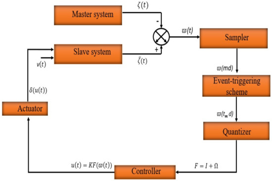
Figure 1.
A schematic representation of the proposed system (4).
The inequality (5) defines the release times , , , etc., where is the initial time. The time between two consecutive release times, , corresponds to the sampling period set by the event generator in (5). The sampling period is bounded below by , and the zero phenomenon is excluded. To determine whether to transmit the current sampled signal, an ET correspondence plan compares the difference between the current sampled sensor measurements and the latest transmitted sensor measurements to a specified threshold given by (5).
A logarithmic quantizer is defined as follows
where . The quantization levels for are given as
where each of the quantization levels is denoted by . The quantizer density is represented by . The initial quantization values of the subquantizer are , where .
The following describes the definition of the logarithmic quantization law denoted by .
where is the quantizer parameters and considering , . Using the method given in [45], due to the symmetry of the logarithmic quantizer, , it can be obtained that the logarithmic quantizer maps are intervals within a quantization level. Note that for
,
and for ,
Thus, the quantizer is characterized as follows:
Then, we can easily get
where , and denotes an uncertain scalar. It is easy to see that .
We now consider the case of time-varying delays in the network communication, denoted by , where is a value that varies over time and belongs to the interval , with being a positive real number. To handle this, we first divide the time interval into subintervals. We then define as follows.
We now consider the following two cases:
Case (i): If , where , define a function as
Obviously,
Case (ii): If , consider the following intervals
To satisfy the ET condition in (5), we introduce two piecewise functions for , as follows:
In case (i), for , define . In case (ii), define
From the above condition, is defined as . It is easy to prove that . Finally, we define .
The quantized controller is defined as
where , is the controller gain matrix to be determined. Since , based on the quantization function, we can write the following:
By utilizing Remark 1, we can determine the impact of actuator saturation on the system being considered at the same time,
From Remark 1, there exists a scalar satisfying:
Therefore, for any , we can derive
Definition 1
([46]). We can use the notation to represent the saturation function of . This function is defined as
where , or we can write it as follows:
Definition 2
([47]). The MJTDNNs (16) are said to be FTS with respect to , if
where and are scalars and satisfy .
Definition 3
([48]). Assume that is a positive stochastic functional, and let us define its weak infinitesimal operator as
Lemma 1
([49]). Assume that ϖ is a differentiable function defined as . Let R be a symmetric matrix in , and let be symmetric matrices. Consider also any matrices and that satisfy
then, the following inequality holds:
where
,
, , .
Lemma 2
([50]). For matrices and , we have
where is any chosen constant.
Lemma 3
((Schur Complement) [50]). The LMI is equivalent to , .
Lemma 4
([51]). Suppose we have , as well as a positive definite matrix . Then, we can state the following inequality
3. Main Results
Based on the above discussions, this section uses a suitable LKF for the error system (16) as FTS under a quantized ET control scheme. For convenience, we establish the following naming conventions for vectors and matrices:
, ,
,
, ,
, ,
,
,
,
,
,
,
,
,
,
,
,
,
,
,
Theorem 1.
where , .
For given scalars , , , , , , , , and time constant , and control gain , the MJTDNNs (16) can achieve stochastic FTS with respect to if the following conditions are satisfied: Symmetric positive-definite matrices , , , , , exist, along with appropriate dimension matrices , , , , , , , , , , , and . Diagonal matrices U and , and scalars (l = 1, 2, …, 7) also exist. The above matrices and scalars must satisfy certain matrix inequalities:
Proof.
Construct the LKF as follows:
where
Consequently, the weak infinitesimal operator of is defined as follows:
Applying the techniques presented in [52], we can obtain an equation for the weak infinitesimal generator of by computing it along the system trajectory, as shown in Equation (16). This can be achieved using the following expression:
By using Lemma 1, we can get
For any appropriate dimension matrix , we can consider the following equality,
Based on Assumption 1, we can write
similarly, we get
where , .
We can obtain the following inequality from Equations (32)–(41), as well as from Equations (13) and (18)
By utilizing the Schur complement (Lemma 3) with Equation (42), we can arrive at the following:
Based on Equation (44), and under the assumption of a positive constant satisfying certain conditions, it follows that
The following inequality can be derived from inequality (45):
It is worth noting that the value of t lies between 0 and T. Utilizing this fact, we can derive the following inequality,
We can obtain the following information by utilizing Equation (30),
Subsequently, we can attain,
from the above inequality, we can obtain
Based on Definition 2, we can determine that the system described by Equation (16) achieves stochastic FTS with respect to . □
Remark 2.
In our approach, we utilized an ET mechanism and free-weighting matrices to derive (16) in Theorem 1. However, due to the presence of condition (5), directly obtaining the gains for (16) is not possible. To address this challenge, we introduce a new theorem that allows us to obtain the gain needed to meet the requirements of the system. This theorem is crucial for enabling us to effectively implement the ET control scheme and ensure the synchronization and performance of the MJTDNNs.
Now, we are in a position to design the ET controller for the error system (16).
Theorem 2.
where
where , .
Suppose we have a time constant and scalars , , , , , , , , and . Let the MJTDNNs (16) be subject to the ET condition (5) and gain matrix . If there exist symmetric positive-definite matrices , , , , , and , as well as appropriately dimensioned matrices , , , , , , , , , (), (), (), and (), as well as diagonal matrices U and , and scalars (), , , , and such that the inequalities for the matrices are as follows, then the MJTDNNs are stochastically FTS with respect to :
Proof.
To prove Theorem 2, we can follow the same approach as in Theorem 1. First, let us define . Next, we can multiply Equations (26)–(29) on the left and right by , respectively. Then, by defining a new matrix variable , we can use Theorem 1 to define the subsequent steps,
For the uncertain terms from (60), , ,
, and there exist scalars , , , and such that
Remark 3.
We already knew that the research object of articles [2,3,53,54] was MJNNs, but we can see that these articles mainly discussed stability, state estimation, and synchronization research. Different from the method of constructing functionals in these articles, this article discusses a kind of FTS with quantization and actuator saturation problems, which is rare. On the other hand, the issue of FTS is also not involved in QMJTDNNs.
Remark 4.
Many existing works with respect to finite-time synchronization conditions for NNs, see [15,16,17], address these in terms of inequalities. Compared with the approach used in [17], the finite-time synchronization conditions obtained in Theorem 2 can be addressed in terms of LMIs, which can be solved by utilizing the LMI toolbox in Matlab. It should be mentioned that condition (31) cannot be solved directly in terms of LMIs; however, by constructing an LKF with free-matrix-based integral inequalities and utilizing Schur complement lemma, the matrix inequalities are turned into the linear matrix inequalities, which can be solved in terms of LMIs.
Remark 5.
By utilizing the novel LKF, more information about the time-delay variation can be incorporated into the synchronization existence conditions. Therefore, compared to the approach presented in [17] and Theorem 2 in this paper, the latter can yield less-conservative results. Fortunately, only the LMIs in Theorem 2 need to be solved, allowing for the establishment of the relationship between neural network synchronization and time delays, although the proposed method with free-weighting matrices and zero inequality has a higher complexity than existing results in [17]. Using the MATLAB LMI toolbox, the calculations are no longer a huge problem. Therefore, compared with existing results, the proposed conditions can still be viewed as an improvement over existing results.
4. Numerical Examples
Example 1.


Consider a two-neuron two-mode MJTDNN (16) with the following system parameters with
and the Markovian process with transition matrix . The delays and the other parameter are given as follows: , , . By solving LMIs (50)–(58), we get ; then, the feasible solutions are as follows:
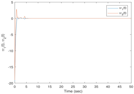
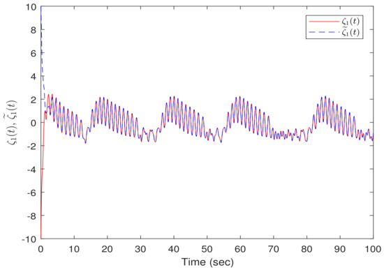
The flowchart of event-triggered control is illustrated in Figure 2. Moreover, the simulation results for Example 1 are presented in Figure 3, Figure 4 and Figure 5. A sampling period of was set, and the initial condition was . Figure 3 and Figure 4 show the evolution of and , respectively, while Figure 5 displays the trajectories of . It is evident from the figures that the system reached a synchronized state for a certain period of time under the action of the controller (14), thus validating the effectiveness of the proposed control method.
Figure 2.
The flowchart of the proposed controller in Example 1.
Figure 3.
The time response of state variable in Example 1.
Figure 4.
The time response of state variable in Example 1.
Figure 5.
The time evolution of the error system states in Example 1.
Table 1 provides a summary of the maximum upper bound (MUB) that is appropriate for each separate μ, as determined by Theorem 2, along with the upgrade values that correspond to those upper bounds. The findings of this research indicate that the method that was suggested is an impactful means of determining the highest permissible upper bound, as shown by the obtained results.
Table 1.
Maximum allowable bound for different values of , for Example 1.
Example 2.


Mode 1:
Mode 2:
Mode 3:
The activation functions are chosen as , which can be easily obtained from Assumption 1.
Assuming that the Markov process is satisfied, the transition matrix for the MJTDNN with three jumping modes specified in Equation (16) can be represented in the following manner:
Here, is the value that we chose to specify as the value of the parameter for the triggered scheme that applied to this scenario. In addition, we specified the following values for the other parameters: , and for the quantization parameter. By utilizing the LMI toolbox available in MATLAB and Theorem 2, we obtained and determined that the ET matrix was given by
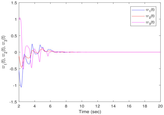
Under the obtained gain matrix of Theorem 2, the conditions are satisfied; then, MJTDNN (16) is FTS, and the simulation results are presented in Figure 6, Figure 7, Figure 8 and Figure 9.
Figure 6.
State responses for in Example 2.
Figure 7.
State responses for in Example 2.
Figure 8.
State responses for in Example 2.
Figure 9.
State trajectories for the error system in Example 2.
Figure 6, Figure 7 and Figure 8 illustrate the state trajectories of the master and slave systems’ state responses, which show that the slave system can track the real states . The initial conditions for the drive and response systems were chosen as and , respectively. Figure 9 plots the trajectory of the error estimation signal where it can be seen that the designed synchronization satisfied the specified requirements, demonstrating the effectiveness of the designed FTS. It is observed from Figure 6, Figure 7, Figure 8 and Figure 9 that the ET controller proposed in the study effectively achieved the FTS between the response system and the master system.
5. Conclusions
This paper studied the problem of an FTS for QMJTDNNs with actuator saturation and an ET strategy. The proposed controller ensured that the synchronization error converged to zero within a finite time while reducing the communication burden among nodes by triggering updates only when necessary. The FTS criteria for QMJTDNNs were derived in the form of LMIs using a suitable LKF. Then, solving the LMIs, the ET control gains were obtained. The effectiveness of the proposed approach was demonstrated through numerical simulations. For future directions, several avenues could be explored. For instance, one could investigate the robustness of the proposed method under various uncertainties or disturbances. Moreover, we could extend the main results in this paper to more realistic systems; for instance, the sliding-mode control with fractional-order reaction–diffusion terms and other network issues, such as dropouts and denial of service (DoS), will be considered for the ET sliding-mode control of the concerned system. From a practical perspective, as network communication continues to evolve and becomes more complex, it will be increasingly important to explore the diverse range of attack methods that may emerge. This will be a key area of focus in our future research, as we aim to develop innovative approaches for detecting and mitigating these threats and enhancing the resilience and security of network communication systems; the proposed approach can be also suitable for other systems such as in [14,16].
Author Contributions
Conceptualization, S.S.; methodology, R.V.; formal analysis, R.V.; investigation, N.G.; writing—original draft, S.S.; writing—review and editing, N.G.; supervision, N.G. and R.V. All authors have read and agreed to the published version of the manuscript.
Funding
This research was funded by the Centre for Nonlinear Systems, Chennai Institute of Technology (CIT), India, with funding number CIT/CNS/2023/RP-005.
Data Availability Statement
Data sharing is not applicable to this article as no datasets were generated or analyzed during the current study.
Acknowledgments
We gratefully acknowledge this work was funded by the Centre for Nonlinear Systems, Chennai Institute of Technology (CIT), India.
Conflicts of Interest
The author declares that there is no conflict of interest regarding the publication of this paper.
References
- Yu, Y.; Zhang, Z.; Zhong, M.; Wang, Z. Pinning synchronization and adaptive synchronization of complex-valued inertial neural networks with time-varying delays in fixed-time interval. J. Frankl. Inst. 2022, 359, 1434–1456. [Google Scholar] [CrossRef]
- Lin, Y.; Zhuang, G.; Xia, J.; Sun, W.; Zhao, J. Asynchronous H∞ dynamic output feedback control for Markovian jump neural networks with time-varying delays. Int. J. Control. Autom. Syst. 2022, 20, 909–923. [Google Scholar] [CrossRef]
- Wu, T.; Cao, J.; Xiong, L.; Zhang, H.; Shu, J. Sampled-data synchronization criteria for Markovian jumping neural networks with additive time-varying delays using new techniques. Appl. Math. Comput. 2022, 413, 126604. [Google Scholar] [CrossRef]
- Zou, C.; Li, B.; Liu, F.; Xu, B. Event-Triggered μ-state estimation for Markovian jumping neural networks with mixed time-delays. Appl. Math. Comput. 2022, 425, 127056. [Google Scholar] [CrossRef]
- Song, X.; Lu, H.; Xu, Y.; Zhou, W. H∞ synchronization of semi-Markovian jump neural networks with random sensor nonlinearities via adaptive event-triggered output feedback control. Math. Comput. Simul. 2022, 198, 1–19. [Google Scholar] [CrossRef]
- Aslam, M.S.; Li, Q.; Hou, J.; Qiulong, H. Mode-dependent delays for dissipative filtering of stochastic semi-Markovian jump for neural networks. Adv. Contin. Discret. Model. 2022, 2022, 21. [Google Scholar] [CrossRef]
- Li, Z.; Zhang, Z.; Liao, Q.; Rong, M. Asymptotic and robust stabilization control for the whole class of fractional-order gene regulation networks with time delays. Fractal Fract. 2022, 6, 406. [Google Scholar] [CrossRef]
- Zhang, S.; Liu, X.; Li, X. Finite-time synchronisation of delayed fractional-order coupled neural networks. Int. J. Syst. Sci. 2022, 53, 2597–2611. [Google Scholar] [CrossRef]
- Li, D.; Cao, J. Finite-time synchronization of coupled networks with one single time-varying delay coupling. Neurocomputing 2015, 166, 265–270. [Google Scholar] [CrossRef]
- Dai, A.; Zhou, W.; Xu, Y.; Xiao, C. Adaptive exponential synchronization in mean square for Markovian jumping neutral-type coupled neural networks with time-varying delays by pinning control. Neurocomputing 2016, 173, 809–818. [Google Scholar] [CrossRef]
- Dorato, P. Short-Time Stability in Linear Time-Varying Systems; Polytechnic Institute of Brooklyn: Brooklyn, NY, USA, 1961. [Google Scholar]
- Weiss, L.; Infante, E. Finite time stability under perturbing forces and on product spaces. IEEE Trans. Autom. Control 1967, 12, 54–59. [Google Scholar] [CrossRef]
- Wang, L.; Shen, Y.; Ding, Z. Finite time stabilization of delayed neural networks. Neural Netw. 2015, 70, 74–80. [Google Scholar] [CrossRef]
- Tang, R.; Su, H.; Zou, Y.; Yang, X. Finite-time synchronization of Markovian coupled neural networks with delays via intermittent quantized control: Linear programming approach. IEEE Trans. Neural Netw. Learn. Syst. 2021, 33, 5268–5278. [Google Scholar] [CrossRef] [PubMed]
- Guan, C.; Fei, Z.; Karimi, H.R.; Shi, P. Finite-time synchronization for switched neural networks via quantized feedback control. IEEE Trans. Syst. Man Cybern. Syst. 2019, 51, 2873–2884. [Google Scholar] [CrossRef]
- Xu, C.; Yang, X.; Lu, J.; Feng, J.; Alsaadi, F.E.; Hayat, T. Finite-time synchronization of networks via quantized intermittent pinning control. IEEE Trans. Cybern. 2017, 48, 3021–3027. [Google Scholar] [CrossRef]
- Zhang, D.; Cheng, J.; Cao, J.; Zhang, D. Finite-time synchronization control for semi-Markov jump neural networks with mode-dependent stochastic parametric uncertainties. Appl. Math. Comput. 2019, 344, 230–242. [Google Scholar] [CrossRef]
- He, W.; Luo, T.; Tang, Y.; Du, W.; Tian, Y.C.; Qian, F. Secure communication based on quantized synchronization of chaotic neural networks under an event-triggered strategy. IEEE Trans. Neural Netw. Learn. Syst. 2019, 31, 3334–3345. [Google Scholar] [CrossRef]
- Sheng, S.; Zhang, X.; Lu, G. Finite-time outer-synchronization for complex networks with Markov jump topology via hybrid control and its application to image encryption. J. Frankl. Inst. 2018, 355, 6493–6519. [Google Scholar] [CrossRef]
- He, X.; Zhang, H. Exponential synchronization of complex networks via feedback control and periodically intermittent noise. J. Frankl. Inst. 2022, 359, 3614–3630. [Google Scholar] [CrossRef]
- Peng, D.; Li, X. Leader-following synchronization of complex dynamic networks via event-triggered impulsive control. Neurocomputing 2020, 412, 1–10. [Google Scholar] [CrossRef]
- Zhang, M.; Zang, H.; Bai, L. A new predefined-time sliding mode control scheme for synchronizing chaotic systems. Chaos Solitons Fractals 2022, 164, 112745. [Google Scholar] [CrossRef]
- Zhao, Y.; Ren, S.; Kurths, J. Synchronization of coupled memristive competitive BAM neural networks with different time scales. Neurocomputing 2021, 427, 110–117. [Google Scholar] [CrossRef]
- Lu, B.; Jiang, H.; Hu, C.; Abdurahman, A.; Liu, M. H∞ output synchronization of directed coupled reaction-diffusion neural networks via event-triggered quantized control. J. Frankl. Inst. 2021, 358, 4458–4482. [Google Scholar] [CrossRef]
- Zhang, Y.; Li, X.; Liu, C. Event-triggered finite-time quantized synchronization of uncertain delayed neural networks. Optim. Control Appl. Methods 2022, 43, 1584–1603. [Google Scholar] [CrossRef]
- Cuomo, K.M.; Oppenheim, A.V.; Strogatz, S.H. Synchronization of Lorenz-based chaotic circuits with applications to communications. IEEE Trans. Circuits Syst. II Analog Digit. Signal Process. 1993, 40, 626–633. [Google Scholar] [CrossRef]
- Zheng, Q.; Xu, S.; Du, B. Quantized guaranteed cost output feedback control for nonlinear networked control systems and its applications. IEEE Trans. Fuzzy Syst. 2021, 30, 2402–2411. [Google Scholar] [CrossRef]
- Li, J.; Niu, Y. Output-feedback-based sliding mode control for networked control systems subject to packet loss and quantization. Asian J. Control 2021, 23, 289–297. [Google Scholar] [CrossRef]
- Xue, B.; Yu, H.; Wang, M. Robust H∞ Output feedback control of networked control systems with discrete distributed delays subject to packet dropout and quantization. IEEE Access 2019, 7, 30313–30320. [Google Scholar] [CrossRef]
- Chang, X.H.; Jin, X. Observer-based Fuzzy feedback control for nonlinear systems subject to transmission signal quantization. Appl. Math. Comput. 2022, 414, 126657. [Google Scholar] [CrossRef]
- Zhao, R.; Zuo, Z.; Wang, Y. Event-triggered control for networked switched systems with quantization. IEEE Trans. Syst. Man Cybern. Syst. 2022, 52, 6120–6128. [Google Scholar] [CrossRef]
- Shanmugam, S.; Hong, K.S. An event-triggered extended dissipative control for Takagi-Sugeno Fuzzy systems with time-varying delay via free-matrix-based integral inequality. J. Frankl. Inst. 2020, 357, 7696–7717. [Google Scholar] [CrossRef]
- Zong, G.; Ren, H. Guaranteed cost finite-time control for semi-Markov jump systems with event-triggered scheme and quantization input. Int. J. Robust Nonlinear Control 2019, 29, 5251–5273. [Google Scholar] [CrossRef]
- Liu, D.; Yang, G.H. Dynamic event-triggered control for linear time-invariant systems with-gain performance. Int. J. Robust Nonlinear Control 2019, 29, 507–518. [Google Scholar] [CrossRef]
- Vadivel, R.; Hammachukiattikul, P.; Zhu, Q.; Gunasekaran, N. Event-triggered synchronization for stochastic delayed neural networks: Passivity and passification case. Asian J. Control 2022. [Google Scholar] [CrossRef]
- Fan, Y.; Huang, X.; Shen, H.; Cao, J. Switching event-triggered control for global stabilization of delayed memristive neural networks: An exponential attenuation scheme. Neural Netw. 2019, 117, 216–224. [Google Scholar] [CrossRef]
- Vadivel, R.; Hammachukiattikul, P.; Gunasekaran, N.; Saravanakumar, R.; Dutta, H. Strict dissipativity synchronization for delayed static neural networks: An event-triggered scheme. Chaos Solitons Fractals 2021, 150, 111212. [Google Scholar] [CrossRef]
- Vadivel, R.; Ali, M.S.; Joo, Y.H. Event-triggered H∞ synchronization for switched discrete time delayed recurrent neural networks with actuator constraints and nonlinear perturbations. J. Frankl. Inst. 2020, 357, 4079–4108. [Google Scholar] [CrossRef]
- Lin, J.; Shi, P.; Xiao, M. Event-triggered stabilisation of sampled-data singular systems: A hybrid control approach. Int. J. Control 2022. [Google Scholar] [CrossRef]
- Fragoso, M.D.; Costa, O.L. A unified approach for stochastic and mean square stability of continuous-time linear systems with Markovian jumping parameters and additive disturbances. SIAM J. Control Optim. 2005, 44, 1165–1191. [Google Scholar] [CrossRef]
- Xing, X.; Yao, D.; Lu, Q.; Li, X. Finite-time stability of Markovian jump neural networks with partly unknown transition probabilities. Neurocomputing 2015, 159, 282–287. [Google Scholar] [CrossRef]
- Lou, X.; Cui, B. Delay-dependent criteria for global robust periodicity of uncertain switched recurrent neural networks with time-varying delay. IEEE Trans. Neural Netw. 2008, 19, 549–557. [Google Scholar] [PubMed]
- Li, L.; Zou, W.; Fei, S. Event-triggered synchronization of delayed neural networks with actuator saturation using quantized measurements. J. Frankl. Inst. 2019, 356, 6433–6459. [Google Scholar] [CrossRef]
- Yue, D.; Tian, E.; Han, Q.L. A delay system method for designing event-triggered controllers of networked control systems. IEEE Trans. Autom. Control 2012, 58, 475–481. [Google Scholar] [CrossRef]
- Fu, M.; Xie, L. The sector bound approach to quantized feedback control. IEEE Trans. Autom. Control 2005, 50, 1698–1711. [Google Scholar]
- Sun, L.; Wang, Y.; Feng, G. Control design for a class of affine nonlinear descriptor systems with actuator saturation. IEEE Trans. Autom. Control 2014, 60, 2195–2200. [Google Scholar] [CrossRef]
- He, S.; Liu, F. Finite-time boundedness of uncertain time-delayed neural network with Markovian jumping parameters. Neurocomputing 2013, 103, 87–92. [Google Scholar] [CrossRef]
- Luan, X.; Liu, F.; Shi, P. Finite-time filtering for non-linear stochastic systems with partially known transition jump rates. IET Control Theory Appl. 2010, 4, 735–745. [Google Scholar] [CrossRef]
- Zeng, H.B.; He, Y.; Wu, M.; She, J. Free-matrix-based integral inequality for stability analysis of systems with time-varying delay. IEEE Trans. Autom. Control 2015, 60, 2768–2772. [Google Scholar] [CrossRef]
- Boyd, S.; El Ghaoui, L.; Feron, E.; Balakrishnan, V. Linear Matrix Inequalities in System and Control Theory; Society for Industrial and Applied Mathematics (SIAM): Philadelphia, PA, USA, 1994. [Google Scholar]
- Wang, Y.; Xie, L.; De Souza, C.E. Robust control of a class of uncertain nonlinear systems. Syst. Control Lett. 1992, 19, 139–149. [Google Scholar] [CrossRef]
- Cheng, J.; Zhu, H.; Ding, Y.; Zhong, S.; Zhong, Q. Stochastic finite-time boundedness for Markovian jumping neural networks with time-varying delays. Appl. Math. Comput. 2014, 242, 281–295. [Google Scholar] [CrossRef]
- Jiang, X.; Xia, G.; Feng, Z.; Jiang, Z.; Qiu, J. Reachable set estimation for Markovian jump neutral-type neural networks with time-varying delays. IEEE Trans. Cybern. 2020, 52, 1150–1163. [Google Scholar] [CrossRef] [PubMed]
- Wu, Z.G.; Shi, P.; Su, H.; Chu, J. Stochastic synchronization of Markovian jump neural networks with time-varying delay using sampled data. IEEE Trans. Cybern. 2013, 43, 1796–1806. [Google Scholar] [CrossRef] [PubMed]


Disclaimer/Publisher’s Note: The statements, opinions and data contained in all publications are solely those of the individual author(s) and contributor(s) and not of MDPI and/or the editor(s). MDPI and/or the editor(s) disclaim responsibility for any injury to people or property resulting from any ideas, methods, instructions or products referred to in the content. |
© 2023 by the authors. Licensee MDPI, Basel, Switzerland. This article is an open access article distributed under the terms and conditions of the Creative Commons Attribution (CC BY) license (https://creativecommons.org/licenses/by/4.0/).