Fractional-Order Variational Image Fusion and Denoising Based on Data-Driven Tight Frame

Abstract

Multi-modal image fusion can provide more image information, which improves the image quality for subsequent image processing tasks. Because the images acquired using photon counting devices always suffer from Poisson noise, this paper proposes a new three-step method based on the fractional-order variational method and data-driven tight frame to solve the problem of multi-modal image fusion for images corrupted by Poisson noise. Thus, this article obtains fused high-quality images while removing Poisson noise. The proposed image fusion model can be solved by the split Bregman algorithm which has significant stability and fast convergence. The numerical results on various modal images show the excellent performance of the proposed three-step method in terms of numerical evaluation metrics and visual quality. Extensive experiments demonstrate that our method outperforms state-of-the-art methods on image fusion with Poisson noise.

1. Introduction

A single image cannot fully display all the information of the target scene. For example, computed tomography (CT) images mainly shows hard bone tissues of the body, while magnetic resonance imaging (MRI) mainly shows soft tissues. Multifocus images are formed by focusing on different objects because the imaging equipment cannot achieve focused imaging of all the objects in the same scene. Infrared images can capture thermal radiation information, but the resolution is poor, while visible images have higher resolution. Therefore, it is essential to perform image fusion. The current research of image fusion is mainly applied in the fields of medical science [1], remote sensing [2], monitoring [3], etc.

The current image fusion algorithms are mainly based on the principal component analysis method [4], the pyramid transform-based method [5], the wavelet transform-based method [6], etc. The article [7] elaborates the theoretical knowledge behind the different fusion algorithms. The method based on principal component analysis is easy-to-understand research. However, it is computationally intensive and has poor real-time performance. The methods based on pyramid transform mainly include the Laplacian pyramid [8], gradient pyramid [9], etc. However, the pyramid decomposition is redundant and lacks direction selectivity, which cannot effectively present the structural information of the fused image and leads to blurred boundaries of the fused image. The main methods based on wavelet transform are dual-tree complex wavelet transform [10], contourlet transform [11], shearlet transform [12], etc., but the relationship between the decomposition layers, fusion quality, and time efficiency need to be balanced. The article [13] describes the latest research progress in image fusion.

Because the variational method has a mature theoretical system and it is easy to design and analyze [14], it is widely used in image recovery [15], image denoising [16], and image fusion [17]. The authors in the literature [15] proposed a variational model for local non-texture inpainting based on the total variational model and the Mumford–Shah model. The authors in the literature [16] proposed a fractional-order total variational model for image denoising. In the literature [17], a three-step method for fusing clear images is proposed, as shown in Figure 1. In the image decomposition step, the images are processed using a variational model based on the data-driven tight frame (DDTF):

$$\begin{array}{c}\hfill \underset{v_1,v_2,{\left\{a_i\right\}}_{i=1}^{r^2}}{min}\parallel v_1-W{u}_1{\parallel }_2^2+\parallel v_2-W{u}_2{\parallel }_2^2+{\lambda }_1^2\parallel v_1{\parallel }_0+{\lambda }_2^2{\parallel v_2\parallel }_0,\end{array}$$

(1)

$$s.t.W^{T}W=I,$$

where ${\lambda }_1>0,{\lambda }_2>0$ are the parameters corresponding to the two balances. $u_1,u_2$ are the clear source images, and $v_1,v_2$ are the sparse representation coefficients of $u_1,u_2$, respectively. $W:=W(a_1,a_2,\dots ,a_{r^2})$ is the analysis operator associated with the tight frame generated by $r^2$ two-dimensional filters ${\left\{a_i\right\}}_{i=1}^{r^2}$. I is the unit matrix. Unfortunately, clear images can be handled by this method; images containing noise do not work.

In addition, noise is also an important factor to be considered in the image fusion process. In the process of actual image generation, noise interference is inevitable. For example, Poisson noise is often generated when using photon counting devices, which mainly depends on the number of photons. The common noises mainly include Gaussian noise, salt and pepper noise, Poisson noise, etc. The first two kinds of noise have been studied by a large number of researchers [18,19,20,21]. Image denoising is performed using artificial neural networks in article [22], and a new hybrid filter technique is proposed by combining anisotropic diffusion with a Butterworth band-pass filter to overcome over-filtering of the image in article [23] for image denoising. Hence, in this paper, we focus on the image disturbed by Poisson noise. The Tikhonov regularization model [22], the total variational model (TV) [23], and the higher-order total variational model [24] are common methods that use variational models for removing Poisson noise. The total variational-based denoising model is as follows:

$$\underset{u}{min}{\parallel \nabla u\parallel }_1+\beta {\parallel u-flnu\parallel }_1.$$

(2)

where $\beta$ is a positive parameter, f is the source image, and u is the denoised image. This model performs well on piecewise constant images, but it causes staircasing artifacts for piecewise smooth images. High-order total variational models such as the PDE-based model [25] and the Lysaker–Lundervold–Tai (LLT) model [26] introduce speckle artifacts.

Different from other types of models, the fractional-order total variational (FOTV) model has shown that it can suppress staircasing artifacts and speckle artifacts [27]. By considering the intensity of adjacent images, their local geometric features can be maintained [28,29]. The literature [16] proposes a Poisson denoising model based on fractional-order total variation, which can maintain the high-order smoothness of the image. The model is as follows:

$$\underset{u}{min}\parallel {\nabla }^{\alpha }{u\parallel }_1+\beta {\parallel u-flnu\parallel }_1.$$

(3)

where $\alpha$ is the fraction that is greater than or equal to 1, f is the noise image, u is the denoised image, and $\beta$ is the parameter of the fidelity term.

Before the fusion of images containing noise, the images are usually pre-processed with noise removal; however, this operation also reduces the efficiency of image fusion. Consider that each term in the variational model (1) for image fusion and the variational model (3) for image denoising is independent and indispensable to each other. The addition of an item to the variational model is feasible and easy to interpret. Many methods have been proposed to simultaneously denoise and fuse images disturbed by Gaussian noise [30,31,32], and these methods have achieved excellent results. Inspired by them, we want to fuse images disturbed by Poisson noise using the variational model.

In this paper, a new three-step method for image denoising and fusion is proposed by combining the two variational models (1) and (3), and its work flowchart is shown in Figure 2. Firstly, in the image decomposition step, an improved variational model is proposed to process the images with noise, and the split Bregman method is used to solve it. Secondly, the coefficients are constructed according to the fusion rules. Finally, the fused image is obtained using the variational model in the image reconstruction step, which maintains the image smoothness and significant features.

Our contributions can be summarized as follows:

• Motivated by a fractional-order total variational denoising model and a data-driven tight frame variational model for image fusion, a variational fusion model capable of handling noisy images is constructed. The denoised images and analysis operator are obtained by this model.
• The new three-step method is constructed. The method combines FOTV and DDTF models for simultaneously denoising and fusing images, and it can find the complementary information from the noisy source images to obtain the final fused images and suppress the noise output. This is the first time that a fractional-order variational model is used to denoise and fuse images disturbed by Poisson noise.
• We evaluate this method on different types of images. The experiments show that the proposed method is more effective.

The rest of this paper is organized as follows. In Section 2, a new three-step method is proposed. In Section 3, the solving procedure using the split Bregman algorithm is described in detail. In Section 4, by numerical experiments, the advantages of the proposed method are illustrated. This paper concludes with a brief summary in Section 5.

2. Materials and Methods

In this section, we focus on the basic theory of fractional-order derivatives and image fusion, and the proposed three-step method is further described.

2.1. Related Materials

Fractional-order derivatives are widely used in image processing due to their extra degrees of freedom. The literature [33] reviews the progress of research on fractional-order derivatives in different image processing areas. Full-reference image quality assessment methods are proposed in the literature [34] by combining the Grünwald–Letnikov derivative and image gradients. The application of fractional-order derivatives in color image edge detection is presented in the literature [35].

Total variation models using fractional-order derivatives are used for Gaussian noise removal [36], Poisson noise removal [16], multiplicative noise removal [37], etc. The theory of fractional-order derivatives is described below. The fractional-order gradient is defined as ${\nabla }^{\alpha }u=[D_1^{\alpha }u,D_2^{\alpha }u]$, where $D_1^{\alpha }u,D_2^{\alpha }u$ are the discrete gradients along the x-axis and the y-axis and are defined by

$${\left(D_1^{\alpha }u\right)}_{i,j}=\sum _{k=0}^{K-1}{(-1)}^k{C}_k^{\alpha }{u}_{i-k,j},{\left(D_2^{\alpha }u\right)}_{i,j}=\sum _{k=0}^{K-1}{(-1)}^k{C}_k^{\alpha }{u}_{i,j-k}.$$

where K is the number of adjacent pixels used to calculate the fractional-order derivative at each pixel. The image u is expressed as a matrix $u_{i,j},1\le i\le N,1\le j\le M$. The coefficients ${\left\{C_k^{\alpha }\right\}}_{k=0}^{K-1}$ are determined by the Gamma function $\mathsf{\Gamma }\left(x\right)$, $C_k^{\alpha }=\frac{\mathsf{\Gamma }(\alpha +1)}{\mathsf{\Gamma }(k+1)\mathsf{\Gamma }(\alpha +1-k)}$. Then, the FOTV of u is defined as

$$\parallel {\nabla }^{\alpha }{u\parallel }_1:=\sum _{i,j}|{\left(D_1^{\alpha }u\right)}_{i,j}|+|{\left(D_2^{\alpha }u\right)}_{i,j}|.$$

Notice that when $\alpha =1$, ${\left(D_1^{1}u\right)}_{i,j}=u_{i,j}-u_{i-1,j},{\left(D_2^{1}u\right)}_{i,j}=u_{i,j}-u_{i,j-1}.$ It is natural that FOTV is equivalent to TV.

The basic idea of image fusion using the variational method is as follows: the actual image problem is first transformed into an energy general function model and then solved by the variational method. The general structure of image fusion is mainly divided into three steps: image decomposition, the fusion coefficient according to certain rules, and image reconstruction. In other words, the source image is first input, and then the fused image is finally output after the whole process. Both the first and third steps use the variational model to process the image, as shown in Figure 2.

2.2. The Proposed New Three-Step Method

For the proposed new three-step method, the specific model corresponding to each step will be introduced in detail. In the step of image decomposition, the model that can process images with Poisson noise is proposed as follows:

$$\begin{array}{cc}\hfill \underset{u_1,u_2,v_1,v_2,{\left\{a_i\right\}}_{i=1}^{r^2}}{min}& {\gamma }_1\parallel u_1-f_{1}ln{u}_1{\parallel }_1+{\gamma }_2\parallel u_2-f_{2}ln{u}_2{\parallel }_1+{\beta }_1\parallel {\nabla }^{\alpha }{u}_1{\parallel }_1+{\beta }_2{\parallel {\nabla }^{\alpha }{u}_2\parallel }_1\hfill \\ \hfill & +\parallel v_1-W{u}_1{\parallel }_2^2+\parallel v_2-W{u}_2{\parallel }_2^2+{\lambda }_1^2\parallel v_1{\parallel }_0+{\lambda }_2^2{\parallel v_2\parallel }_0,\hfill \end{array}$$

(4)

$$s.t.W^{T}W=I,$$

where ${\gamma }_1,{\gamma }_2,{\beta }_1,{\beta }_2,{\lambda }_1,{\lambda }_2$ are the parameters, which are all positive values. The last two items using ${\lambda }_1^2,{\lambda }_2^2$ are convenient to solve with the hard threshold operator. $f_1,f_2$ are the images containing noise, $u_1,u_2$ are the denoised images, $v_1,v_2$ are the sparse representation coefficients of $u_1,u_2$, and W is the analysis operator.

By solving the model (4), the denoised images $u_1,u_2$ and the analysis operator W are obtained. We use $c_i=W{u}_i$ to denote the coefficients of the image $u_i$, $i=1,2$. The magnitude of the coefficients at each pixel can indicate the presence or absence of features in the neighborhood of that pixel, and the fusion coefficients are represented by the following fusion rule:

$$c^j\left(x\right)=\left\{\begin{array}{c}{c}_1^j\left(x\right),x\in \left\{x\right|{\Sigma }_j|c_1^j\left(x\right)|\ge {\Sigma }_j|c_2^j\left(x\right)\left|\right\},\hfill \\ c_2^j\left(x\right),x\in \left\{x\right|{\Sigma }_j|c_1^j\left(x\right)|<{\Sigma }_j|c_2^j\left(x\right)\left|\right\},\hfill \end{array}\right.$$

(5)

where $c^j\left(x\right)$ denotes the coefficient of the jth filter acting at pixel x, $j=1,2,\dots ,r^2,x=1,2,\dots ,N$. $c_i^j\left(x\right)$ denotes the coefficients of the jth filter acting at pixel x of images $u_i$, $i=1,2$.

For the image reconstruction step, based on the denoised images $u_1,u_2$ and coefficients c obtained in the first two steps, the fused image u is reconstructed using the following variational model:

$$\underset{u}{min}{\parallel Wu-c\parallel }_1+\frac{{\mu }_1}{2}{\parallel u|}_{{\mathrm{\Omega }}_1}-u_1{|}_{{\mathrm{\Omega }}_1}{\parallel }_2^2+\frac{{\mu }_2}{2}{\parallel u|}_{{\mathrm{\Omega }}_2}-u_2{{|}_{{\mathrm{\Omega }}_2}\parallel }_2^2,$$

(6)

where ${\mu }_1,{\mu }_2$ are parameters, ${\mathrm{\Omega }}_i$ denotes the restricted area of $u_i$, ${\mathrm{\Omega }}_i=\left\{j\right||\nabla u\left(j\right)|<t\}$, and t is a constant.

3. Algorithm

In this section, the models (4) and (6) corresponding to the image decomposition and image reconstruction steps are described in detail.

3.1. Image Decomposition

For the variational model (4) proposed in the previous section, it is equal to the following subproblems.

• The u-subproblem: for fixed $W,v_1,v_2$, we solve

  $$\underset{u_1}{min}{\gamma }_1\parallel u_1-f_{1}ln{u}_1{\parallel }_1+{\beta }_1\parallel {\nabla }^{\alpha }{u}_1{\parallel }_1+{\parallel v_1-W{u}_1\parallel }_2^2,$$

  (7)

  $$\underset{u_2}{min}{\gamma }_2\parallel u_2-f_{2}ln{u}_2{\parallel }_1+{\beta }_2\parallel {\nabla }^{\alpha }{u}_2{\parallel }_1+{\parallel v_2-W{u}_2\parallel }_2^2.$$

  (8)
• The v-subproblem: for fixed $W,u_1,u_2$, we solve

  $$\underset{v_1,v_2}{min}\parallel v_1-W{u}_1{\parallel }_2^2+\parallel v_2-W{u}_2{\parallel }_2^2+{\lambda }_1^2\parallel v_1{\parallel }_0+{\lambda }_2^2{\parallel v_2\parallel }_0.$$

  (9)
• The W-subproblem: for fixed $v_1,v_2,u_1,u_2$, we solve

  $$\underset{W^{T}W=I}{min}\parallel v_1-W{u}_1{\parallel }_2^2+{\parallel v_2-W{u}_2\parallel }_2^2.$$

  (10)

Firstly, the u-subproblem is solved by introducing the variables $Q_1={\nabla }^{\alpha }{u}_1,Q_2={\nabla }^{\alpha }{u}_2$ and taking the split Bregman iteration method to transform Equations (7) and (8) into the following form:

$$\begin{array}{cc}\hfill (u_1^{k+1},Q_1^{k+1})=& \underset{u_1,Q_1}{argmin}{\gamma }_1\parallel u_1-f_{1}ln{u}_1{\parallel }_1+{\beta }_1\parallel Q_1{\parallel }_1+{\parallel v_1^{k+1}-W^{k+1}{u}_1\parallel }_2^2\hfill \\ & +\frac{{\delta }_1}{2}{\parallel Q_1-{\nabla }^{\alpha }{u}_1-{\theta }_1^k\parallel }_2^2,\hfill \end{array}$$

(11)

$${\theta }_1^{k+1}={\theta }_1^k+({\nabla }^{\alpha }{u}_1^{k+1}-Q_1^{k+1}),$$

(12)

$$\begin{array}{cc}\hfill (u_2^{k+1},Q_2^{k+1})=& \underset{u_2,Q_2}{argmin}{\gamma }_2\parallel u_2-f_{2}ln{u}_2{\parallel }_1+{\beta }_2\parallel Q_2{\parallel }_1+{\parallel v_2^{k+1}-W^{k+1}{u}_2\parallel }_2^2\hfill \\ & +\frac{{\delta }_2}{2}{\parallel Q_2-{\nabla }^{\alpha }{u}_2-{\theta }_2^k\parallel }_2^2,\hfill \end{array}$$

(13)

$${\theta }_2^{k+1}={\theta }_2^k+({\nabla }^{\alpha }{u}_2^{k+1}-Q_2^{k+1}),$$

(14)

where the parameters ${\delta }_1,{\delta }_2$ are positive numbers. It is natural that Equations (11) and (13) can be further rewritten as subproblems for $u_1,Q_1,u_2,Q_2$.

$$u_1^{k+1}=\underset{u_1}{argmin}{\gamma }_1\parallel u_1-f_{1}ln{u}_1{\parallel }_1+\parallel v_1^{k+1}-W^{k+1}{u}_1{\parallel }_2^2+\frac{{\delta }_1}{2}{\parallel Q_1^k-{\nabla }^{\alpha }{u}_1-{\theta }_1^k\parallel }_2^2,$$

(15)

$$Q_1^{k+1}=\underset{Q_1}{argmin}{\beta }_1\parallel Q_1{\parallel }_1+\frac{{\delta }_1}{2}{\parallel Q_1-{\nabla }^{\alpha }{u}_1^{k+1}-{\theta }_1^k\parallel }_2^2,$$

(16)

$$u_2^{k+1}=\underset{u_2}{argmin}{\gamma }_2\parallel u_2-f_{2}ln{u}_2{\parallel }_1+\parallel v_2^{k+1}-W^{k+1}{u}_2{\parallel }_2^2+\frac{{\delta }_2}{2}{\parallel Q_2^k-{\nabla }^{\alpha }{u}_2-{\theta }_2^k\parallel }_2^2,$$

(17)

$$Q_2^{k+1}=\underset{Q_2}{argmin}{\beta }_2\parallel Q_2{\parallel }_1+\frac{{\delta }_2}{2}{\parallel Q_2-{\nabla }^{\alpha }{u}_2^{k+1}-{\theta }_2^k\parallel }_2^2.$$

(18)

The Euler–Lagrange equations of Equations (15) and (17) are as follows:

$${\gamma }_1(u_1-f_1)/u_1-2{\left(W^{k+1}\right)}^T(v_1^{k+1}-W^{k+1}{u}_1)-{\delta }_1{\left({\nabla }^{\alpha }\right)}^T(Q_1^k-{\nabla }^{\alpha }{u}_1-{\theta }_1^k)=0,$$

(19)

$${\gamma }_2(u_2-f_2)/u_2-2{\left(W^{k+1}\right)}^T(v_2^{k+1}-W^{k+1}{u}_2)-{\delta }_2{\left({\nabla }^{\alpha }\right)}^T(Q_2^k-{\nabla }^{\alpha }{u}_2-{\theta }_2^k)=0.$$

(20)

To efficiently solve nonlinear Equations (19) and (20), u in the denominator replaces the previous iteration $u^k$ and $u^{k+1}$ is solved by the fast Fourier transform (FFT) under periodic boundary conditions.

$$u_1^{k+1}={\mathcal{F}}^{-1}[\frac{\mathcal{F}(2{\left(W^{k+1}\right)}^T{u}_1^k{v}_1^{k+1}+{\gamma }_1{f}_1+{\delta }_1{\left({\nabla }^{\alpha }\right)}^T{u}_1^k(Q_1^k-{\theta }_1^k))}{{\gamma }_1+\mathcal{F}(2{\left(W^{k+1}\right)}^T{W}^{k+1}{u}_1^k+{\delta }_1{\left({\nabla }^{\alpha }\right)}^T\left({\nabla }^{\alpha }\right)u_1^k)}],$$

(21)

$$u_2^{k+1}={\mathcal{F}}^{-1}[\frac{\mathcal{F}(2{\left(W^{k+1}\right)}^T{u}_2^k{v}_2^{k+1}+{\gamma }_2{f}_2+{\delta }_2{\left({\nabla }^{\alpha }\right)}^T{u}_2^k(Q_2^k-{\theta }_2^k))}{{\gamma }_2+\mathcal{F}(2{\left(W^{k+1}\right)}^T{W}^{k+1}{u}_2^k+{\delta }_2{\left({\nabla }^{\alpha }\right)}^T\left({\nabla }^{\alpha }\right)u_2^k)}],$$

(22)

where $\mathcal{F}$ denotes FFT.

One can verify readily that the solution of subproblem $Q_1,Q_2$ can be expressed explicitly as

$$Q_1^{k+1}=({\nabla }^{\alpha }{u}_1^{k+1}+{\theta }_1^k)max\{0,1-\frac{{\beta }_1}{{\delta }_1|{\nabla }^{\alpha }{u}_1^{k+1}+{\theta }_1^k|}\},$$

(23)

$$Q_2^{k+1}=({\nabla }^{\alpha }{u}_2^{k+1}+{\theta }_2^k)max\{0,1-\frac{{\beta }_2}{{\delta }_2|{\nabla }^{\alpha }{u}_2^{k+1}+{\theta }_2^k|}\}.$$

(24)

By Equations (11)–(24), the solution of the u-subproblem is found. The solution process for the v-subproblem is described below.

Equation (9) can be solved by the hard threshold operator T:

$$v_i^{k+1}=T_{{\lambda }_i}\left(W^k{u}_i^k\right)=\left\{\begin{array}{c}{W}^k{u}_i,\left|W^k{u}_i^k\right|>{\lambda }_i,\hfill \\ 0,|W^k{u}_i^k|\le {\lambda }_i,\hfill \end{array}\right.$$

(25)

where ${\lambda }_i>0$ are given constants, $i=1,2$.

At the end of the image decomposition step, the W-subproblem is solved. Because the subproblem (10) is a minimization problem with quadratic constraints, it can be solved by singular value decomposition (SVD) as follows:

$$W=\frac{1}{r}R{L}^T,$$

(26)

where L, R are the SVD of $V_1{U}_1^T+V_2{U}_2^T$, $V_1{U}_1^T+V_2{U}_2^T=LD{R}^T$. $V_i, U_i$ denotes the matrix that pulls the image blocks of $r\times r$ into column vectors.

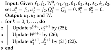
Combining the above solving process, the image decomposition step algorithm is as follows (Algorithm 1):

Algorithm 1: The image decomposition step algorithm

3.2. Image Reconstruction

By introducing the variables $y,z$ and the parameter $\delta >0$, Equation (6) can be solved using the split Bregman iteration method and rewritten as

$$u^{k+1}=\underset{u}{argmin}\frac{{\mu }_1}{2}{\parallel u|}_{{\Omega }_1}-u_1{|}_{{\Omega }_1}{\parallel }_2^2+\frac{{\mu }_2}{2}{\parallel u|}_{{\Omega }_2}-u_2{|}_{{\Omega }_2}{\parallel }_2^2+\frac{\delta }{2}{\parallel Wu-c-z^k+y^k\parallel }_2^2,$$

(27)

$$z^{k+1}=\underset{z}{argmin}{\parallel z\parallel }_1+\frac{\delta }{2}{\parallel z-W{u}^{k+1}+c-y^k\parallel }_2^2,$$

(28)

$$y^{k+1}=y^k+(W{u}^{k+1}-c-z^{k+1}).$$

(29)

Similarly, the solution of the above subproblems can be obtained:

$$u^{k+1}=[\frac{({\mu }_1{D}_1{u}_1+{\mu }_2{D}_2{u}_2+\delta W^T(c+z^k-y^k))}{({\mu }_1{D}_1+{\mu }_2{D}_2+\delta I)}],$$

(30)

$$z^{k+1}=(W{u}^{k+1}-c+y^k)max\{0,1-\frac{1}{\delta |W{u}^{k+1}-c+y^k\left|\right\}}.$$

(31)

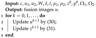
Therefore, the algorithm for image reconstruction is as follows (Algorithm 2):

Algorithm 2: The algorithm for image reconstruction

4. Numerical Experiments

In this section, to verify the effectiveness of the method, numerical experiments of the proposed three-step method are performed. All experimental results were achieved using Matlab (R2016b) on a laptop with Intel(R) Core(TM) i5-1035G1 CPU @ 1.00 GHz 1.19 GHz, 16 GB RAM, Windows 11. Different types of images are selected, including synthesized images [17], medical images [32], multifocused images [38], and infrared and visible images [39], all of which are widely used in image processing.

4.1. Evaluation Metrics

It is important to choose the metrics to evaluate the quality of the denoised image and the fused image. In general, the metrics of the denoising and fusion effect can be divided into two aspects: subjective visual effect and objective quantitative evaluation. The subjective visual effect is that people evaluate the image quality by visual observation, which cannot be judged very accurately. Usually, some objective evaluations are described in the literature. There are many metrics for image evaluation quality, such as an intelligent model proposed in article [40] to evaluate noise in ultrasound images. In this paper, the peak signal-to-noise ratio (PSNR), mutual information (MI) [41], edge strength ($Q_{abf}$) [42], and structural similarity ($Q_e$) [43] are chosen to evaluate the image quality. The PSNR is used to measure the denoising effect of the image. MI is used to measure the amount of information of an image containing another image. $Q_{abf}$ is used to determine the relative amount of edge information that is transferred from the input images into the fused image. $Q_e$ is used for determining the structural similarity between two images. It is characteristic that the larger these values are, the better the results.

4.2. Selection of Parameters

The selection of parameters is crucial in the implementation of the algorithm. In the image decomposition step, the stop criterion is $\frac{\parallel u^{k+1}-u^k{\parallel }_2}{\parallel u^k{\parallel }_2}<{10}^{-5}$, and in the image reconstruction step, the number of iterations is 1000. The method proposed in this paper mainly involves the following parameters. Basic guidance for setting these parameters is discussed. ${\gamma }_1,{\gamma }_2$ are the coefficients of the approximation term. The larger ${\gamma }_1,{\gamma }_2$, the closer the approximation solution obtained is to the exact solution. The parameters ${\beta }_1,{\beta }_2$ are the coefficients of the regular term. The larger ${\beta }_1,{\beta }_2$, the smoother the image obtained; the smaller ${\beta }_1,{\beta }_2$, the denoising effect on the image is not significant. ${\delta }_1$ and ${\delta }_2$ control the penalty function terms of $u_1,u_2$. $\frac{{\beta }_1}{{\delta }_1}$ and $\frac{{\beta }_2}{\delta 2}$ control the iterations of $Q_1,Q_2$.

4.3. Numerical Experimental Results and Analysis

At present, most researchers have studied the simultaneous denoising and fusion of images disturbed by Gaussian noise [36,44,45], and some others have studied the problem of Poisson denoising. There are few studies on the simultaneous denoising fusion of images interfered with by Poisson noise. We found a paper [46] on the simultaneous denoising and fusion of images with Poisson noise, which proposes an online convolutional coding model to train noisy images. The fusion was performed on multifocused images with a PSNR value of 29.46. Because the authors ran the model in GPU, this paper is not compared with it.

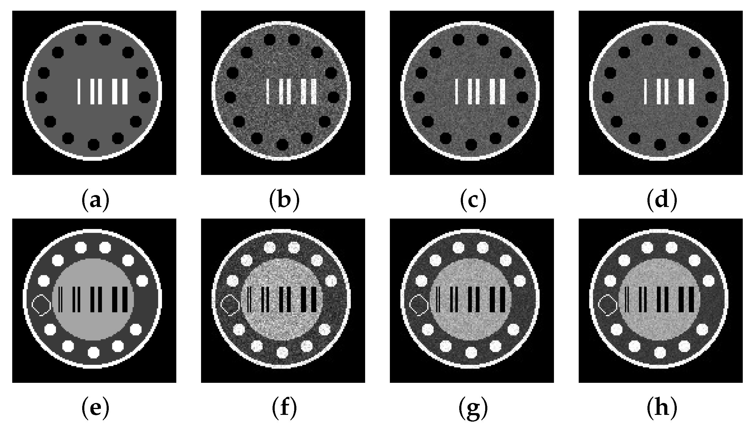
Because Poisson noise depends on the pixel intensity, the noise level can be controlled by the peak intensity of the original image. The original image with a preset peak value is scaled, before adding Poisson noise. Specifically, we consider three peak values: 55, 155, and 255.

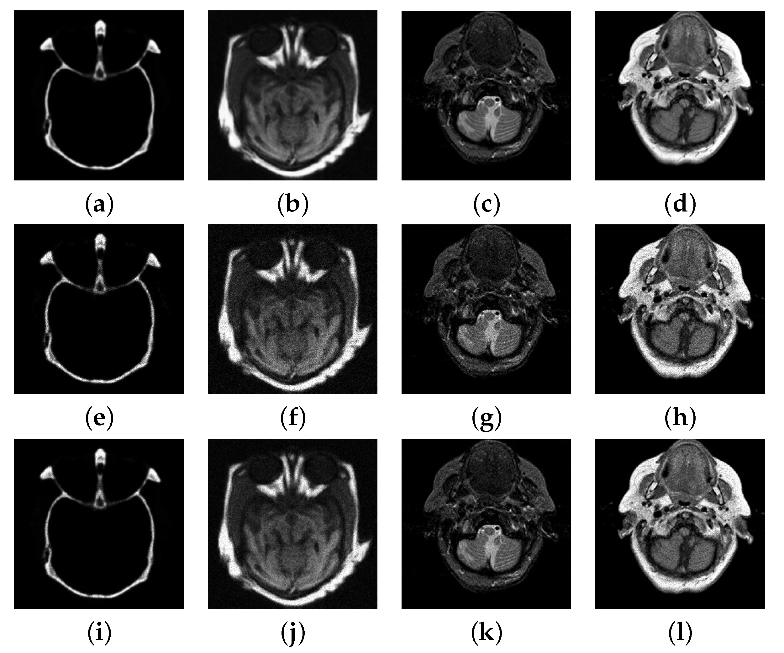
It is obvious from Figure 3 that the image with peak value 55 is more noisy than the image with peak values 155 and 255.

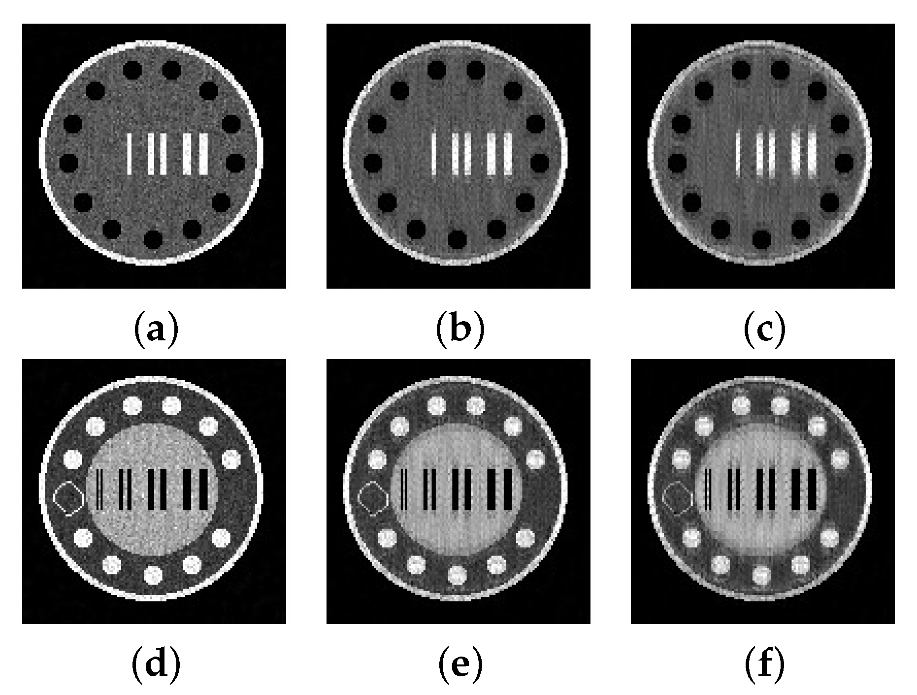
Next, the validity of fractional-order $\alpha$ is verified. In Figure 4, we present the denoising results for the image with peak 55 using different fractional orders $\alpha =1$, 1.6, and 2.4. It is obvious that when $\alpha =1$, i.e., TV, the first column still contains some noise. When $\alpha =2.4$, the last column image is too smooth and blurs the boundary. This means that the fractional-order $\alpha$ has an effect on the final result.

In the following, the numerical experiments on the proposed method using different types of images are performed, i.e., Figure 5, Figure 6, Figure 7, Figure 8, Figure 9, Figure 10, Figure 11 and Figure 12.

In all the experiments, the most appropriate parameters are chosen from the set of parameters ${\gamma }_i\in \{10,{10}^2,5\times {10}^2,8\times {10}^2,{10}^3\}$, ${\beta }_i\in \{3\times {10}^1,5\times {10}^1,8\times {10}^1,{10}^2,5\times {10}^2,8\times {10}^2,{10}^3\}$, and ${\delta }_i\in \{{10}^{-1},{10}^{-2},2\times {10}^{-2},{10}^{-3},5\times {10}^{-3}\}$, $i=1,2$. Firstly, we process the two medical images at peaks 55 and 155 and set $\alpha$ = 1.6, K = 16, and the results are shown in Figure 6.

In Figure 6, the proposed method is very effective for medical images. The Poisson noise in the image is effectively removed and most of the feature information is retained without edge blurring. Information is provided on objective evaluation metrics, i.e., the values of $PSNR$, $MI$, $Q_{abf}$, and $Q_e$ in

Table 1. Indexes of the proposed methods for medical images at peak values 55 and 155, respectively.

Test Images	Peak	Noisy	PSNR	$\mathbf{MI}$	${\mathit{Q}}_{\mathbf{abf}}$	${\mathit{Q}}_{\mathit{e}}$
CT/MRI	55	31.17/24.39	31.70/26.79	1.83	0.50	0.56
	155	35.70/28.85	36.06/28.95	2.55	0.59	0.48
MR-T1/MR-T2	55	27.98/23.90	29.91/26.15	2.61	0.40	0.53
	155	32.41/28.40	32.86/28.29	3.16	0.47	0.41

, which show that the proposed method is more effective in most cases. Note that both ‘Noisy’ and ‘PSNR’ in Table 1,

Table 2. Indexes of the proposed methods for multifocus images at peak values 155 and 255, respectively.

Test Images	Peak	Noisy	PSNR	$\mathit{MI}$	${\mathit{Q}}_{\mathbf{abf}}$	${\mathit{Q}}_{\mathit{e}}$
Multifocus1	155	25.97/25.72	28.02/27.50	4.00	0.40	0.39
	255	28.17/27.87	29.13/28.35	4.58	0.39	0.41
Multifocus2	155	25.39/25.41	29.72/30.16	4.71	0.54	0.70
	255	27.57/27.56	30.43/30.55	4.77	0.60	0.66

,

Table 3. Indexes of the proposed methods for multifocus images at peak values 155 and 255, respectively.

Method	Index	CT/MRI	MR-T1/MR-T2	Multifocus1	Multifocus2
proposed	$MI$	2.51	3.11	4.32	4.69
	$Q_{abf}$	0.59	0.39	0.39	0.54
	$Q_e$	0.44	0.37	0.48	0.69
DDTF	$MI$	2.63	2.72	3.49	3.54
	$Q_{abf}$	0.46	0.40	0.37	0.47
	$Q_e$	0.33	0.28	0.25	0.46

and

Table 4. Indexes of the proposed methods for infrared and visible images at peak values 155 and 255, respectively.

Test Images	Peak	Noisy	PSNR	$\mathit{MI}$	${\mathit{Q}}_{\mathbf{abf}}$	${\mathit{Q}}_{\mathit{e}}$
IR1/VIS1	155	26.71/26.70	27.72/28.89	2.18	0.23	0.40
	255	28.90/29.21	29.29/30.47	2.62	0.24	0.41
IR2/VIS2	155	25.01/25.80	27.63/28.30	1.67	0.29	0.24
	255	27.18/28.00	28.61/29.57	2.12	0.31	0.23

represent the values of the PSNR for the two noisy images and the denoised images, respectively.

Then, the effect of different values of the parameters on the fusion results are discussed, as shown in Figure 7. It is observed that the selection of ${\gamma }_1,{\gamma }_2,{\beta }_1,{\beta }_2$ will affect the final fusion effect, and these parameters are sensitive. The parameters ${\delta }_1,{\delta }_2$ will affect the time of the whole calculation process.

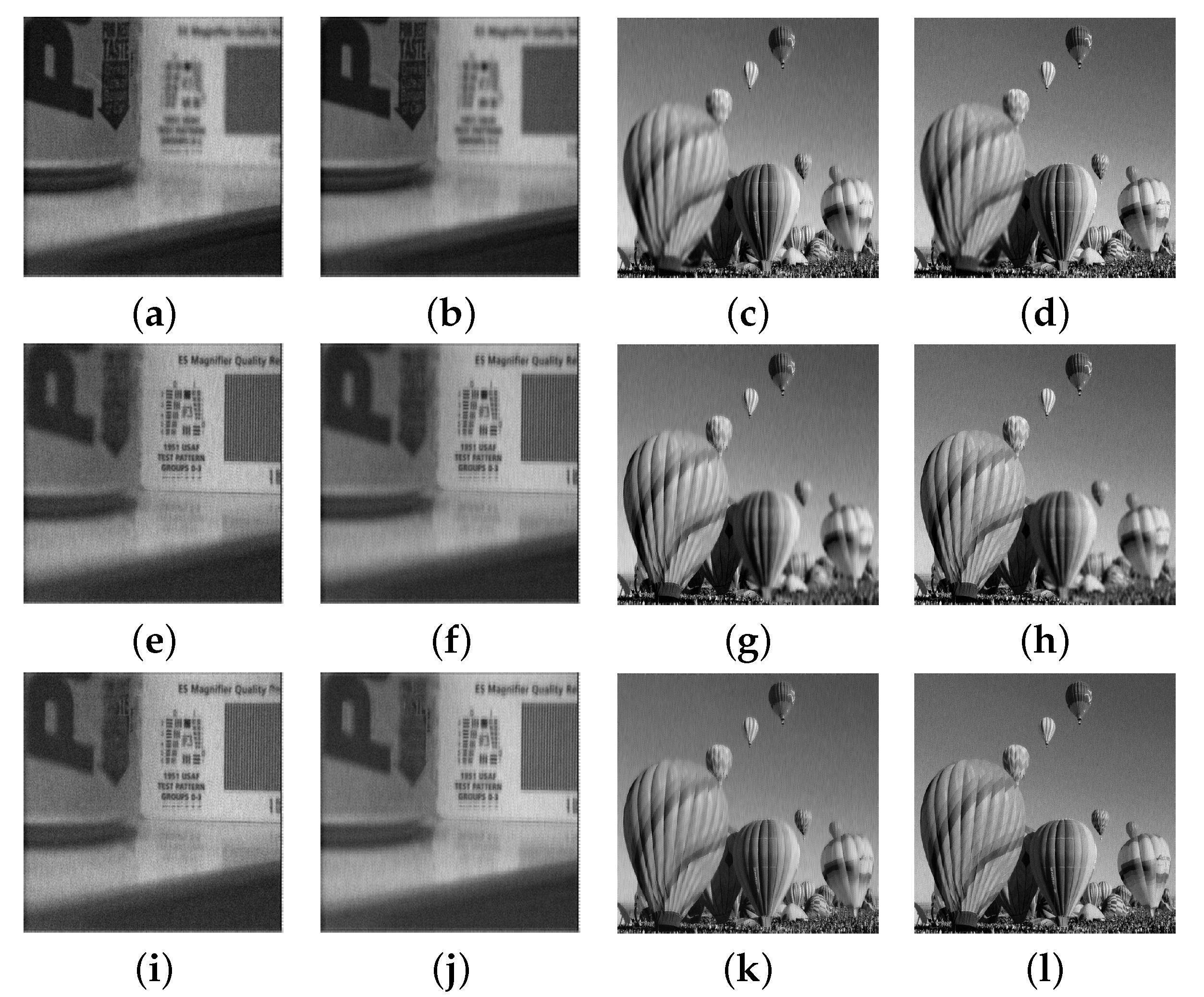
The denoising results and the final fusion results of the multifocus images are described in Figure 8 and Figure 9. Figure 8 shows the multifocus image at peaks of 155 and 255. Figure 9 shows the denoising results and the final fusion results of the multifocus image with peaks of 155 and 255, respectively.

It is not difficult to find that for (a,e,b,f) in Figure 9, although some of the noise can be removed from this image, there is still some left, and the fusion results show that the tiny texture features are blurred, which is consistent with the results in Table 2.

Medical images and multifocal images are used to compare the proposed method with the method in the literature [17], and the results are shown below. In Figure 10, the first row presents the fused images using the proposed method, and the second row presents the fused images using the DDTF method. By looking at these images, it is easy to see that our proposed method has better performance with respect to denoising, which is also illustrated by the values in Table 3.

At the end of the experiment, we show the denoising and fusion results of the infrared and visible images. Figure 11 shows the images at peaks of 155 and 255. Figure 12 shows the denoising results and fusion results for the infrared and visible images at peaks of 155 and 255, respectively.

As can be seen from Figure 12, the proposed method does not seem to be too effective in denoising infrared and visible light, and the fused image still contains some noise, which is consistent with the results in Table 4.

5. Conclusions

In this paper, motivated by the respective advantages of the image fusion method based on the variational model and the denoising method based on the fractional-order variational model, a new three-step method is proposed for the denoising and fusion of images disturbed by Poisson noise. The proposed method is solved by the split Bregman iterative algorithm. The validity of the fractional order in the variational model is examined using synthesis images. In addition, numerical experiments are performed for three different types of images to demonstrate the effectiveness of the method.

References

1. Yang, Y.; Cao, S.; Wan, W.; Huang, S. Multi-modal medical image super-resolution fusion based on detail enhancement and weighted local energy deviation. Biomed. Signal Process. Control 2023, 80, 104387. [Google Scholar] [CrossRef]
2. Gharbia, R.; Hassanien, A.; El-Baz, A.; Elhoseny, M.; Gunasekaran, M. Multi-spectral and panchromatic image fusion approach using stationary wavelet transform and swarm flower pollination optimization for remote sensing applications. Future Gener. Comput. Syst. 2018, 88, 501–511. [Google Scholar] [CrossRef]
3. Paramanandham, N.; Rajendiran, K. Infrared and visible image fusion using discrete cosine transform and swarm intelligence for surveillance applications. Infrared Phys. Technol. 2018, 88, 13–22. [Google Scholar] [CrossRef]
4. Nandi, D.; Ashour, A.; Samanta, S.; Chakraborty, S.; Salem, M.; Dey, N. Principal component analysis in medical image processing: A study. Int. J. Image Min. 2015, 1, 65–86. [Google Scholar] [CrossRef]
5. Du, J.; Li, W.; Xiao, B. Anatomical-functional image fusion by information of interest in local laplacian filtering domain. IEEE Trans. Image Process. 2017, 26, 5855–5866. [Google Scholar] [CrossRef] [PubMed]
6. Prakash, O.; Park, C.; Khare, A.; Jeon, M.; Gwak, J. Multiscale fusion of multimodal medical images using lifting scheme based biorthogonal wavelet transform. Optik 2019, 182, 995–1014. [Google Scholar] [CrossRef]
7. Hermessi, H.; Mourali, O.; Zagrouba, E. Multimodal medical image fusion review: Theoretical background and recent advances. Signal Process 2021, 183, 108036. [Google Scholar] [CrossRef]
8. Burt, P.; Adelson, E. The Laplacian pyramid as a compact image code. Readings Comput. Vision. 1983, 31, 532–540. [Google Scholar] [CrossRef]
9. Petrovic, V.; Xydeas, C. Gradient-based multiresolution image fusion. IEEE Trans. Image Process. 2004, 13, 228–237. [Google Scholar] [CrossRef]
10. Ioannidou, S.; Karathanassi, V. Investigation of the dual-tree complex and shift-invariant discrete wavelet transforms on quickbird image fusion. IEEE Geosci. Remote. Sens. Lett. 2007, 1, 166–170. [Google Scholar] [CrossRef]
11. Yang, L.; Guo, B.; Ni, W. Multimodality medical image fusion based on multiscale geometric analysis of contourlet transform. Neurocomputing 2008, 72, 203–211. [Google Scholar] [CrossRef]
12. Wang, L.; Li, B.; Tian, L. Multi-modal medical image fusion using the inter-scale and intra-scale dependencies between image shift-invariant shearlet coefficients. Inf. Fusion 2014, 19, 20–28. [Google Scholar] [CrossRef]
13. Singh, S.; Singh, H.; Bueno, G.; Deniz, O.; Singh, S.; Monga, H.; Hrisheekesha, P.N.; Pedraza, A. A review of image fusion: Methods, applications and performance metrics. Digit. Signal Process. 2023, 137, 104020. [Google Scholar] [CrossRef]
14. Chan, T.; Shen, J.; Vese, L. Variational PDE models in image processing. Not. Am. Math. Soc. 2003, 50, 14–26. [Google Scholar]
15. Chan, T.; Shen, J. Mathematical models for local non-texture inpainting. SIAM J. Appl. Math. 2002, 62, 1019–1043. [Google Scholar]
16. Rahman, M.; Zhang, J.; Qin, J.; Lou, Y. Poisson image denoising based on fractional-order total variation. Inverse Probl. Imaging 2020, 14, 77–96. [Google Scholar] [CrossRef]
17. Zhang, Y.; Zhang, X. Variational bimodal image fusion with data-driven tight frame. Inf. Fusion 2020, 55, 164–172. [Google Scholar] [CrossRef]
18. Thakur, R.K.; Maji, S.K. Multi scale pixel attention and feature extraction based neural network for image denoising. Pattern Recognit. 2023, 141, 109603. [Google Scholar] [CrossRef]
19. Zhang, Q.; Huang, C.; Yang, L.; Yang, Z. Salt and pepper noise removal method based on graph signal reconstruction. Digit. Signal Process. 2023, 135, 103941. [Google Scholar] [CrossRef]
20. Singh, A.; Kushwaha, S.; Alarfaj, M.; Singh, M. Comprehensive overview of backpropagation algorithm for digital image denoising. Electronics 2022, 11, 1590. [Google Scholar] [CrossRef]
21. Kushwaha, S.; Singh, R.K. Optimization of the proposed hybrid denoising technique to overcome over-filtering issue. Biomed. Eng. Biomed. Tech. 2019, 64, 601–618. [Google Scholar]
22. Tikhonov, A.; Goncharsky, A.; Stepanov, V.; Yagola, A. Numerical Methods for the Solution of Ill-Posed Problems; Mathematics and its Applications; Kluwer Academic Publishers Group: Dordrecht, The Netherlands, 1995; 328p. [Google Scholar]
23. Rudin, L.; Osher, S.; Fatemi, E. Nonlinear total variation based noise removal algorithms. Phys. Nonlinear Phenom. 1992, 60, 259–268. [Google Scholar] [CrossRef]
24. Chan, T.; Marquina, A.; Mulet, P. High-order total variation-based image restoration. SIAM J. Sci. Comput. 2000, 22, 503–516. [Google Scholar] [CrossRef]
25. Zhang, J.; Ma, M.; Wu, Z.; Deng, C. High-order total bounded variation model and its fast algorithm for Poissonian image restoration. Math. Probl. Eng. 2019, 2019, 1–11. [Google Scholar] [CrossRef]
26. Lysaker, M.; Lundervold, A.; Tai, X. Noise removal using fourth-order partial differential equation with applications to medical magnetic resonance images in space and time. IEEE Trans. Image Process. 2003, 12, 1579–1590. [Google Scholar] [CrossRef] [PubMed]
27. Bai, J.; Feng, X. Fractional-order anisotropic diffusion for image denoising. IEEE Trans. Image Process. 2007, 16, 2492–2502. [Google Scholar] [CrossRef] [PubMed]
28. Pu, Y. Fractional differential analysis for texture of digital image. J. Algorithms Comput. Technol. 2007, 1, 357–380. [Google Scholar]
29. Zhang, J.; Chen, K. A total fractional-order variation model for image restoration with nonhomogeneous boundary conditions and its numerical solution. SIAM J. Imaging Sci. 2015, 8, 2487–2518. [Google Scholar] [CrossRef]
30. Liu, L.; Xu, L.; Fang, H. Infrared and visible image fusion and denoising via l2-lp norm minimization. Signal Process. 2020, 172, 107546. [Google Scholar] [CrossRef]
31. Goyal, S.; Singh, V.; Rani, A.; Yadav, N. Multimodal image fusion and denoising in NSCT domain using CNN and FOTGV. Biomed. Signal Process. Control. 2022, 71, 103214. [Google Scholar] [CrossRef]
32. Li, X.; Zhou, F.; Tan, H. Joint image fusion and denoising via three-layer decomposition and sparse representation. Knowl.-Based Syst. 2021, 224, 107087. [Google Scholar] [CrossRef]
33. Yang, Q.; Chen, D.; Zhao, T.; Chen, Y. Fractional calculus in image processing: A review. Fract. Calc. Appl. Anal. 2016, 19, 1222–1249. [Google Scholar] [CrossRef]
34. Varga, D. Full-Reference image quality assessment based on Grünwald–Letnikov derivative, image gradients, and visual saliency. Electronics 2022, 11, 559. [Google Scholar] [CrossRef]
35. Henriques, M.; Valério, D.; Gordo, P.; Melicio, R. Fractional-order colour image processing. Mathematics 2021, 9, 457. [Google Scholar] [CrossRef]
36. Mei, J.; Dong, Y.; Huang, T. Simultaneous image fusion and denoising by using fractional-order gradient information. J. Comput. Appl. Math. 2019, 351, 212–227. [Google Scholar] [CrossRef]
37. Ullah, A.; Chen, W.; Khan, M.A. A new variational approach for restoring images with multiplicative noise. Comput. Math. Appl. 2016, 71, 2034–2050. [Google Scholar] [CrossRef]
38. Jiang, Q.; Jin, X.; Chen, G.; Lee, S.; Cui, X.; Yao, S.; Wu, L. Two-scale decomposition-based multifocus image fusion framework combined with image morphology and fuzzy set theory. Inf. Sci. 2020, 541, 442–474. [Google Scholar] [CrossRef]
39. Li, H.; Wu, X.; Kittler, J. Infrared and visible image fusion using a deep learning framework. In Proceedings of the International Conference on Pattern Recognition, Beijing, China, 20–24 August 2018; pp. 2705–2710. [Google Scholar]
40. Hossain, M.M.; Hasan, M.M.; Rahim, M.A.; Rahman, M.M.; Yousuf, M.A.; Al-Ashhab, S.; Akhdar, H.F.; Alyami, S.A.; Azad, A.; Moni, M.A. Particle swarm optimized fuzzy CNN with quantitative feature fusion for ultrasound image quality identification. IEEE J. Transl. Eng. Health Med. 2022, 10, 1–12. [Google Scholar]
41. Qu, G.; Zhang, D.; Yan, P. Information measure for performance of image fusion. Electron. Lett. 2002, 38, 313–315. [Google Scholar] [CrossRef]
42. Piella, G.; Heijmans, H. A new quality metric for image fusion. In Proceedings of the IEEE International Conference on Image Processing, Barcelona, Spain, 14–17 September 2003; Volume 3, p. III-173. [Google Scholar]
43. Xydeas, C.; Petrovi, V. Objective image fusion performance measure. Electron. Lett. 2000, 36, 308–309. [Google Scholar] [CrossRef]
44. Zhao, W.; Lu, H. Medical image fusion and denoising with alternating sequential filter and adaptive fractional order total variation. IEEE Trans. Instrum. Meas. 2017, 66, 2283–2294. [Google Scholar] [CrossRef]
45. Wang, G.; Li, W.; Du, J.; Xiao, B.; Gao, X. Medical image fusion and denoising algorithm based on a decomposition model of hybrid variation-sparse representation. IEEE J. Biomed. Health Inform. 2022, 26, 5584–5595. [Google Scholar] [CrossRef] [PubMed]
46. Wang, W.; Xia, X.; He, C.; Ren, Z.; Wang, T.; Lei, B. A Noise-Robust online convolutional coding model and its applications to poisson denoising and image fusion. Appl. Math. Model. 2021, 95, 644–666. [Google Scholar] [CrossRef]
Figure 1. The three-step method.
Mathematics 11 02260 g001
Figure 2. The proposed new three-step method.
Mathematics 11 02260 g002
Figure 3. The four columns (ah) of images are synthesized images and the noisy images of peak values at 55, 155, and 255.
Mathematics 11 02260 g003
Figure 4. The three columns (af) of images are the denoised images with peak value 55 at fractional orders 1, 1.6, and 2.4, respectively.
Mathematics 11 02260 g004
Figure 5. (a) CT, (b) MRI, (c) MR-T1, (d) MR-T2. (eh), (il) are the noisy images at peaks of 55 and 155, respectively.
Mathematics 11 02260 g005
Figure 6. The four columns (al) are the denoised image and fused images obtained by processing the medical images at the peak of 55 and 155, respectively.
Mathematics 11 02260 g006
Figure 7. Compare the fusion effect of different parameter values for the noisy image with a peak of 55. Column 1: γ 1 = γ 2 = 10 3 , 5 × 10 2 . Column 2: β 1 = β 2 = 30 , 100 . Column 3: δ 1 = δ 2 = 10 3 , 10 1 .
Mathematics 11 02260 g007
Figure 8. (a) Multifocus1a, (b) Multifocus1b, (c) Multifocus2a, (d) Multifocus2b. (eh), (il) are the noisy images at peaks of 155 and 255, respectively.
Mathematics 11 02260 g008
Figure 9. The four columns (al) are the denoised image and fused images obtained by processing the multifocus images at the peak of 155 and 255, respectively.
Mathematics 11 02260 g009
Figure 10. The two columns (ah) show the fused images obtained by the DDTF method and the proposed method for the image with a peak of 155, respectively.
Mathematics 11 02260 g010
Figure 11. (a) IR1, (b) VIS1, (c) IR2, (d) VIS2. (e)–(h), (il) are the noisy image at peaks of 155 and 255, respectively.
Mathematics 11 02260 g011
Figure 12. The four columns (al) are the denoised image and fused images obtained by processing the infrared and visible images at peaks of 155 and 255, respectively.
Mathematics 11 02260 g012