How Connected Is China’s Systemic Financial Risk Contagion Network?—A Dynamic Network Perspective Analysis

Abstract

Modeling the effects and paths of systemic financial risk contagion is significant for financial stability. This paper focuses on China’s systemic financial risk from the perspective of dynamic networks. First, we construct a high-dimensional dynamic financial network model to capture risk contagion effects. Second, considering the ripple effect of financial risk contagion, we introduce and improve the basic model of the ripple-spreading network. Finally, small- and medium-sized banks and economic policy uncertainty are selected as the internal and external contagion source, respectively, to simulate the risk of ripple-spreading paths. The results show that financial contagion is more likely to occur within the same industry. The contagion triggered by internal shock first spreads within the same industry, and then to other industries. The contagion triggered by external shock first spreads to banks, then to diversified financial institutions, securities and insurance institutions, successively. Moreover, some small- and medium-sized commercial banks show strong abilities to spread risk ripples. The securities industry is the intermediary layer of the ripple network and plays a leading role in the ripple-spreading process. Therefore, systemic financial risk regulation should focus not only on large financial institutions but also on financial institutions with strong ripple effects. During major risk events, isolating risk intermediary nodes can cut off the paths of risk contagion and mitigate the impact on the whole financial system effectively.

1. Introduction

Systemic financial risk prevention and control is a common concern in all countries and academic circles. In recent years, the downward pressure on the economy at home and abroad has increased, and the risk factors are intertwined and superimposed. Various “black swan” events and “grey rhinoceros” factors have aggravated the uncertainty of the global economic and financial system and its systemic risk. The recent bankruptcy of Silicon Valley Bank has renewed global fears of a new round of financial turmoil [1]. However, with the deepening of global integration, the financial crisis is no longer just a problem in developed markets, and the financial network and systemic risk in emerging markets are also worthy of attention. As the functional core of the modern economy, China’s financial system faces increasing sources of turbulence and potential risk points. On the one hand, banks, securities, insurance and the diversified financial institutions have developed complex business and numerous financial products, which make China’s financial system show higher connectedness and a proclivity to risk contagion. On the other hand, financial system in China is simultaneously exposed to external shocks such as public health events, international financial market volatility and economic policy uncertainty, etc. Accompanied by exogenous shocks and endogenous influences, the derivative and contagion paths of systemic financial risk show networked characteristics. Therefore, modeling the effects and paths of systemic risk contagion in China is of great significance to maintain the stability of Chinese financial system and even the world economy.

The structure of the financial network is constantly developing and evolving, and the impact of financial risk events on the financial system is also a dynamic conduction process. When the financial system is affected by macroeconomic shocks, economic system reforms or some unpredictable factors, the equilibrium state of the original network structure will be broken, and the intensity, form and direction of risk contagion may change. Therefore, the financial network structure is always in an unstable state, and it is unreasonable to use the static model to analyze the network contagion relationship. Granger [2] pointed out that structural instability is a non-negligible problem in the field of economic research and that static models have difficulty capturing structural changes in sample relationships. Bostanci et al. [3] also showed that static network models could not reflect the shift in the role of risk contagion relationships across time. Therefore, we focus on the dynamic modeling of the financial network. The rolling time window technology is often used to capture the time-varying characteristic of financial networks [4,5], which is advantageous in describing the differences of financial network risk contagion relationships in different periods. In particular, since the financial system is characterized by high dimensionality and high complexity, how to integrate the “high-dimensional” and “time-varying” characteristics of financial network into the same framework and construct the high-dimensional dynamic network model is worth further exploration.

Ripple effect describes the phenomenon of an effect caused by one thing spreading gradually. That is, if one of the related things changes, the others will follow; just like throwing a stone into a lake, the ripples will spread from the center to the surroundings and gradually spread into the distance. Existing studies have shown that systemic financial risk contagion has ripple effects [6,7]. When the contagion source causes financial contagion, financial risks will spread in the financial system gradually and dynamically, and then affect the stability and security of the whole financial system [8]. In fact, the formation and evolution of many real complex network systems largely depend on the spreading of the influence of a few local events, which have similar behavior rules as the ripple-spreading phenomenon in nature. The ripple-spreading network model (RSNM) [9,10] is the result of the study of the natural ripple-spreading phenomenon, which can simulate the dynamic process of the initial ripple spreading by setting the relevant behavioral parameters. Jie et al. [11] proposed a dynamic ripple-spreading algorithm for solving optimization problems in random network. In addition, the natural ripple-spreading process of RSNM has certain similarities with financial risk contagion characteristics such as the initial ripple energy value in the model corresponding to the magnitude of financial shocks; the energy amplification coefficient corresponding to the risk amplifying effect of institutions; the connection threshold corresponding to risk resistance ability of institutions, etc. Therefore, the dynamic contagion paths of systemic financial risk in a financial network can be better described by simulating the laws embodied in the natural ripple-spreading phenomenon.

This paper aims to reveal the networked contagion mechanisms of China’s systemic financial risk from the perspective of dynamic network. How to build a high-dimensional dynamic financial network to capture risk contagion effects? How to extract and integrate the factors influencing financial contagion to study risk ripple-spreading process? How to construct a ripple-spreading network model that is consistent with the characteristics of financial risk contagion? We focus on answering the above questions. In addition, it should be noted that we explore the risk characteristics of the financial system at the whole system level, focusing on financial risk with systemic hazards, that is, once an institution suffers from an internal or external shock and goes bankrupt, other financial institutions will also suffer losses or even go bankrupt as a result. Therefore, this risk is a systemic risk, which is essentially different from the financial institutions’ own risk.

This paper is organized as followsL Section 2 offers a brief related literature review. Section 3 describes the methodology. Section 4 presents data and the empirical analysis results. Section 5 provides a brief conclusion.

2. Related Literature

The networked contagion characteristics of systemic financial risk have made complex network techniques a mainstream approach to studying systemic financial risk.

Existing studies on systemic financial risk contagion from the perspective of complex networks was mainly divided into two main categories: one was the financial network constructed based on actual business data; the other was the financial network constructed based on high-frequency market data. The first type of financial networks mainly included interbank payment networks [12,13], common risk exposure networks [14,15], asset-liability networks [16,17], etc. Such financial networks reflected the bilateral transactions of financial institutions based on the actual asset correlation relationships, and could better identify risk contagion paths. However, most of the required asset data was difficult to obtain and update in real time, which led to the lag in monitoring systemic risk and was not suitable for the dynamic financial network construction [18].

In recent years, an increasing number of scholars have constructed financial complex network models based on financial market data and portrayed the global risk contagion effects among sectors. Benoit et al. [18] pointed out that the measurement of systemic financial risk based on market data was not confined to a specific correlation form among individuals and could realize the global and multi-channel measurement research on systemic financial risk. Mao et al. [19] pointed out that the network approach is more suitable for presenting a virtually spatial structure of financial networks. Related studies in this field mainly included correlation networks [20,21], causal networks [22,23,24], information spillover networks [25,26] and tail risk networks [27,28,29]. In addition to these common financial networks, many novel networks had been developed to study financial contagion such as multilayer networks [30,31], Bayesian networks [32], multiplex networks [33], etc. Among them, the network connectedness approach proposed by Diebold et al. [25] broke the limitation of measuring the risk spillover relationship between variables in the “two-two” framework and could consider the multi-period influence relationship between variables, which had certain advantages over other financial network models. However, most relevant studies were carried out in the traditional low-dimensional framework. Demirer et al. [34] pointed out that when the number of variables in the VAR system increases, the network connectedness approach would face the problem of the “ dimensional curse “, which was difficult to apply to the study of complex risk contagion relationships among multiple institutions or markets. With the continuous development of modern econometric methods, the application of LASSO and elastic network shrinkage technology provided the possibility for the construction of high-dimensional financial networks [35]. In particular, the elastic network shrinkage technology combines LASSO and ridge regression, which had better efficacy in the estimation of high-dimensional dynamic network models based on the rolling time window [5].

To sum up, the studies of systemic financial risk contagion from the perspective of complex networks has yielded relatively rich results. In these financial networks, nodes represent financial institutions or financial markets, edges represent inter-individual correlations, and the contagion effects and paths of systemic risk can be identified by measuring and testing whether there are correlation, causality or spillover effects between network nodes. In addition, some scholars pay attention to the high-dimensional financial network. However, throughout the studies in this field, there is little literature on modeling and analyzing the dynamic ripple-spreading process of systemic financial risk contagion. Thus, in considering and integrating relevant factors affecting financial risk contagion, we propose using the ripple-spreading network model to simulate financial contagion. The risk ripple-spreading processes show the dynamic paths of financial contagion, and reveal which financial institutions are first infected with financial contagion and which are later infected, thus providing a new tool for the regulatory practice of systemic risk.

3. Methodology

3.1. High-Dimensional Dynamic Network Model of Systemic Risk Contagion

The Diebold–Yilmaz Connectedness Index (DYCI) method links forecast error variance decompositions to edge weights in networks, providing a network estimate [25]. However, when the number of variables in the VAR system increases, it will face the problem of the “dimensional curse “. To overcome this problem, we adopt the elastic network shrinkage technology to estimate the sparse VAR of financial institution volatilities. Gross et al. [5] pointed out that for the estimation of a high-dimensional dynamic network model based on the rolling time window, the elastic network shrinkage technology has a stronger applicability. The implementation of the DYCI model starts with the estimation of an N-variable VAR (p) model:

$$X_t={\displaystyle {\sum }_{ k=1}^{ p}{\beta }_k}{X}_{t-k}+{\epsilon }_{\mathrm{t}}$$

(1)

where $X_t={(x_{1,t},x_{2,t},\dots ,x_{N,t})}^{\prime }$ is an N-dimensional endogenous variable; ${\beta }_k$ is the $N\times N$ coefficients matrix to be estimated. The elastic network shrinkage estimation will solve the following optimization problem:

$$\widehat{\beta }=\arg {\min }_{\beta }\left\{{\displaystyle {\sum }_{ t=1}^{ T}{(X_{it}-{\displaystyle {\sum }_{ k=1}^{ p}{\beta }_{k,i}{X}_{it-k}})}^2+\lambda {\displaystyle {\sum }_{ k=1}^{ p}[(1-\alpha )\left|{\beta }_{k,i}\right|+\alpha {\left|{\beta }_{k,i}\right|}^2]}}\right\}$$

(2)

where $\widehat{\beta }$ is the estimated coefficient matrix of the elastic network; $(1-\alpha )\left|{\beta }_{k,i}\right|+\alpha {\left|{\beta }_{k,i}\right|}^2$ is the penalty function, $0\le \alpha \le 1$. When $\alpha =0$, the penalty function is LASSO form. When $\alpha =1$, the model is transformed into ridge regression form. Parameter $\lambda$ controls the penalty intensity. In this paper, we use the “10-fold cross-validation” to determine the values of parameters $\alpha$ and $\lambda$ based on the principle of minimizing the mean square error.

The variance decomposition matrix gives an intuitive and appealing measure of edge weights: what proportion of future fluctuations in variable $i$ results from the shocks in variable $j$. The pairwise connectedness ${\theta }_{i\leftarrow j}^H$ can be calculated as follows:

$${\theta }_{i\leftarrow j}^H=\frac{{\mathsf{\sigma }}_{ii}^{-1}{\displaystyle {\sum }_{h=0}^{H-1}{(e_i^{\prime }{A}_h\sum e_j)}^2}}{{\displaystyle {\sum }_{h=0}^{H-1}{(e_i^{\prime }{A}_h\sum A_h^{\prime }{e}_i)}^2}}$$

(3)

where ${\mathsf{\sigma }}_{ii}^{-1}$ is the standard deviation of the error term for the $i$th equation; $A_h$ is $h$-step moving average coefficient matrix; $e_i$ is the selection vector, with one as the $i$th element and zeros otherwise. Since the shocks are not orthogonal, the entries of each row in the variance decomposition matrix do not add up to 1. Hence, to better analyze the risk contagion effect, we normalize it based on a row summation approach in order to obtain the following:

$$X_{i\leftarrow j}^H=({\theta }_{i\leftarrow j}^H/{\displaystyle {\sum }_{j=1}^N{\theta }_{i\leftarrow j}^H})\times 100$$

(4)

Further, following Diebold et al. [25], we can look at more aggregate measures such as “to connectedness” and “from connectedness”. Where “to connectedness” denotes the total directional connectedness from variable $i$ to all remaining variables, “from connectedness” denotes the total directional connectedness to variable $i$ from all remaining variables. Additionally, “aggregate connectedness” measures the total effect of risk spillover in the financial system. They are denoted by $S_i^H(to)$, $S_i^H(from)$ and $S(H)$, respectively, as follows:

$$S_i^H(to)=X_{j\leftarrow i}^H; S_i^H(from)=X_{i\leftarrow j}^H , i\ne j$$

(5)

$$S(H)=\frac{1}{N}{\displaystyle {\sum }_{i,j=1}^N{X}_{j\leftarrow i}^H}=\frac{1}{N}{\displaystyle {\sum }_{i, j=1}^N{X}_{i\leftarrow j}^H}, i\ne j$$

(6)

Further, to refine the risk cross-contagion effect within and between sectors, we group the four sectors of banking, securities, insurance and diversified financial industries, and calculate OUT, IN, OTO (out-to-other) and IFO (in-from-other) indicators for each institution in the group.

$$OU{T}_i=\frac{1}{N-1}{\displaystyle {\sum }_{j=1}^N{X}_{j\leftarrow i}} ; I{N}_i=\frac{1}{N-1}{\displaystyle {\sum }_{j=1}^N{X}_{i\leftarrow j}} , i\in a , i\ne j$$

(7)

$$OT{O}_i=\frac{1}{N-N_a}{\displaystyle {\sum }_{j=1}^{N-N_a}{X}_{j\leftarrow i}^H} ; IF{O}_i=\frac{1}{N-N_a}{\displaystyle {\sum }_{j=1}^{N-N_a}{X}_{i\leftarrow j}^H},i\in a,j\notin a$$

(8)

where $OU{T}_i$ represents the average risk output intensity of financial institution $i$ to the system network; $I{N}_i$ represents the intensity of financial institution $i$ exposure to system network shocks; $a$ denotes the group, which can be banking, securities, insurance or the diversified financial industry. $OT{O}_i$ and $IF{O}_i$ denote the average risk output intensity of institution $i$ in group $a$ to all individuals in other groups, and the average risk shock intensity received from all individuals in other groups, respectively; $N_a$ indicates the number of members in group $a$. By comparing the mean values of $OT{O}_i$ and $IF{O}_i$ in each group, the risk contagion roles of different financial sectors can be identified. When OTO-mean > IFO-mean, this group is the net risk output sector; when OTO-mean < IFO-mean, this group is the net risk input sector.

Finally, the $G{I}_{a\to b}$ (Group Influence) indicator is calculated to portray the intensity of risk cross-contagion among the sectors in each group.

$$G{I}_{a\to b}=\frac{1}{N_a{N}_b}{\displaystyle {\sum }_{i=1}^{N_a}{\displaystyle {\sum }_{j=1}^{N_b}{X}_{i\to j}^H}}, i\in a,j\in b$$

(9)

where financial institution $i$ belongs to group $a$, institution $j$ belongs to group $b$; $N_a$ and $N_b$ denote the number of members in group $a$ and group $b$, respectively.

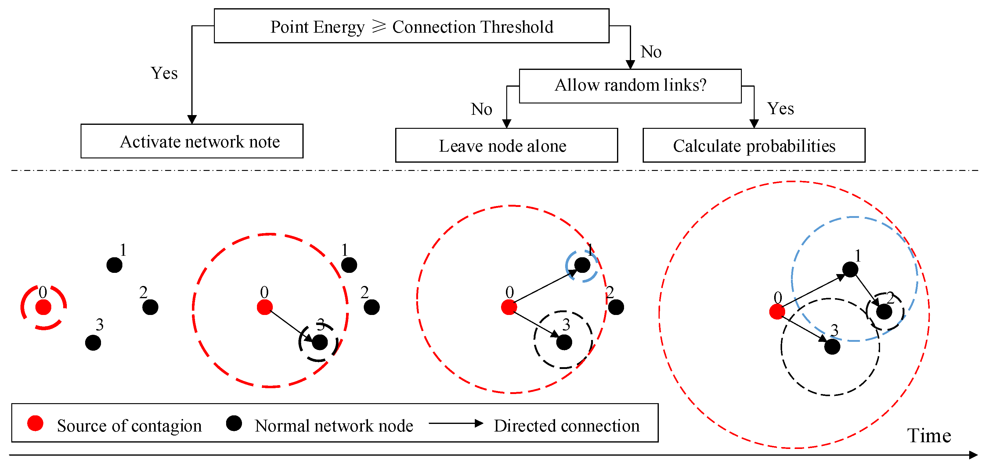
3.2. Ripple-Spreading Network Model of Systemic Risk Contagion

The ripple-spreading network model (RSNM) proposed by Hu et al. [9] is the result of the study of the natural ripple-spreading phenomenon. The core of the RSNM is to determine the parameters of ripple-spreading behavior, which include the contagion source-related parameters and the network node-related parameters.

(1) The contagion source-related parameters are $E_0$, $s_0$ and $d_{0i}$.

$E_0$: The energy of the initial ripple triggered by the contagion source;

$s_0$: The spreading speed of the ripple triggered by contagion source;

$d_{0i}$: The distance between the contagion source and node $i$.

(2) The node-related parameters are ${\alpha }_i$, ${\beta }_i$, $s_i$ and $d_{ij}$.

${\alpha }_i$: The risk amplifying factor of node $i$;

${\beta }_i$: The connection threshold, representing the resistance of node $i$ to shocks;

$s_i$: The spreading speed of the ripple triggered by note $i$;

$d_{ij}$: The distance between node $i$ and $j$.

The RSNM model has a very good potential for both extensions and applications, and can accurately describe the network topology using easily manageable ripple-spreading related parameters, which is more memory efficient than traditional adjacency matrix. The ripple-spreading network model constructed by Hu et al. [9] is a deterministic ripple-spreading network, i.e., given a set of parameters, the final topological structure can be uniquely determined. However, in the process of financial risk contagion, the determinants and uncertainties exist simultaneously. The risk of a financial institution or asset is triggered both by its own characteristics such as the ability of the financial institution to resist risk contagion and by many unknown factors such as market sentiment that cause financial risks to propagate in a more or less unpredictable manner. Uncertainty itself is especially an essential feature of financial risk contagion. Thus, in order to better coordinate the determinants and uncertainties in the risk system, we introduce some stochastic features and construct the semi-deterministic model based on the deterministic model to simulate systemic financial risk contagion spreading process, i.e., if the current point energy of the stimulating ripple is above the connection threshold of a node, then the node behavior must occur. Further, in the case where no threshold of the node is reached, the node may still be activated according to a certain probability function.

Following Hu et al. [9], Figure 1 below gives the basic idea of the semi-deterministic ripple-spreading network model in a simple and intuitive form.

Specifically, based on the ripple behavior parameters, the new ripple-spreading network model can be described as the following dynamic simulation process:

Step 1: Initialize the current time instant, i.e., $t=0$.

Initialize the current point energy of contagion source as $e_{source}(t)=E_0,(E_0>0)$. Since each node has no initial energy, i.e., $E_{nodes}(i)=0$, its current point energy is $e_{nodes}(i,t)=E_{nodes}(i)=0, i=1,2,\cdots ,N$. Assume contagion source and each node has a ripple with a current radius of 0, i.e., $r_{source}(i,t)=0$, $r_{nodes}(i,t)=0$.

Step 2: If the stopping criteria is not satisfied, let $t=t+1$.

Then, update the current radius and point energy of contagion source as follows:

$$r_{source}(i,t)=r_{source}(i,t-1)+s_0 ; e_{source}(i,t)=f_{Decay}(E_0,r_{source}(i,t))$$

(10)

where $s_0$ is the spreading speed of ripples caused by contagion source, and $f_{Decay}$ is a function defining how the point energy decays as the ripple spreads out.

A typical decaying function can be defined as follows:

$$f_{Decay}(E_0,r_{source}(i,t))=\frac{\eta E_0}{2\pi r_{source}(i,t)}$$

(11)

where $\eta$ is a decaying coefficient and $\pi$ is the mathematical constant. Clearly, $\eta$ has an important influence on the decaying speed of ripples, and will therefore affect the final network topology. In this paper, we set $\eta =1$.

Step 3: Check which new nodes are reached by the ripples of contagion source. If $d_{0j}\le r_{source}(i,t)$, then the initial ripple spreads to node $j$. If $d_{0j}>r_{source}(i,t)$, and the initial ripple fails to spread to node $j$, which needs to be reached at $t+2$ or further moments.

Step 4: Check which new nodes are activated and generate response ripples. If $e_{source}(i,t)\ge {\beta }_j$, then node $j$ is activated and generates a responding ripple, thus creating a directed connection from the contagion source to node $j$. At this point, node $j$ generates a responding ripple with initial energy $E_{nodes}(j)={\alpha }_j{e}_{source}(i,t)$.

Further, initialize the current point energy of the response ripple to $e_{nodes}(j,t)=E_{nodes}(j)$, and update the current radius and point energy of the ripple starting from node $j$ in a similar way to contagion source, i.e.,

$$r_{nodes}(i,t)=r_{nodes}(i,t-1)+s_i ; e_{nodes}(i,t)=f_{Decay}(E_N(i),r_{nodes}(i,t))$$

(12)

In this step, we consider the uncertainty characteristics of financial risk contagion. If $e_{source}(i,t)<{\beta }_j$, then node $j$ will generate responding ripple with the following probability, where ${\omega }_R>0$ is the probability decay coefficient. Obviously, the lower the ripple energy, the lower the probability of generating node behavior.

$$P_R(j)=2^{{\omega }_R\left(1-{\beta }_R(j)/e_{source}(i,t)\right)}$$

(13)

Step 5: Check which new nodes are reached by the ripples of other nodes. If $d_{ij}\le r_{nodes}(i,t)$, then node $j$ is reached by the ripple generated by node $i$. If $e_{nodes}(i,t)\ge {\beta }_j$, then node $j$ is activated by node $i$, and generates a responding ripple with $E_{nodes}(j)={\alpha }_j{e}_{nodes}(i,t)$. Then, a directed connection between node $i$ and node $j$ is established, i.e., $A(i,j)=1$, where $A$ is the adjacency matrix which records the network topology. Likewise, we consider the uncertainty characteristics of financial risk contagion. If $e_{nodes}(i,t)<{\beta }_j$, then node $j$ generates responding ripple with the following probability.

$$P_R(j)=2^{{\omega }_R\left(1-{\beta }_R(j)/e_{nodes}(i,t)\right)}$$

(14)

Step 6: Repeat step 5 until the upper time limit T is reached. Clearly, in the semi-deterministic ripple-spreading network model, the final network topology has one part of connections completely determined by ripple-spreading parameters, while the other part of connections are generated in a relatively random way.

4. Empirical Results and Analysis

4.1. Sample Selection and Data Description

In order to ensure sufficient and representative samples, 44 financial institutions listed before 2011 are selected, as shown in

Table 1. Name and abbreviation of financial institution.

Institution Name	Abbr.	Institution Name	Abbr.	Institution Name	Abbr.
Industrial and Commercial Bank of China	ICBC	Bank of Ningbo	BNB	China Life Insurance	CLIC
Agricultural Bank of China	ABC	China Merchants Securities	CMS	China Pacific Insurance	CPIC
Bank of China	BOC	Changjiang Securities	CJS	China Ping An Insurance	PAIC
China Construction Bank	CCB	CITIC securities	CITIC	Tianmao Insurance Company	TMIC
Bank of Communications	BCM	Everbright Securities	EBS	Xinli Finance	XLF
China Merchants Bank	CMB	GF securities	GFS	Anxin Trust and Investment	AXT
Shanghai Pudong Development Bank	SPD	Guoyuan Securities	GYS	Bohai Leasing	BHL
China CITIC Bank	BCC	Sinolink securities	SLS	Luxin Venture Capital	LXC
Ping An Bank	PAB	Southwest Securities	SWS	Minmetals Capital Company	MCC
Huaxia Bank	HXB	Haitong Securities	HTS	Minsheng Holdings	MSH
China Minsheng Bank	MSB	Huatai Securities	HZS	Aijian Group	AJG
China Everbright Bank	CEB	Northeast Securities	NES	Shaanxi International Turst	SIT
China’s Industrial Bank	IBC	Pacific Securities	PS	Sunny Loan Top	SLT
Bank of Beijing	BOB	Sealand Securities	SS	Cnpc Capital Company Limited	CNP
Bank of Nanjing	BNJ	Industrial Securities	IS

, including banks, securities, insurance and diversified financial institutions. The sample covers the periods from 4 January 2011 to 10 February 2023, with a total of $44\times 2940$ samples. Following Demirer et al. [34], we use the stock volatility of financial institutions for empirical research and analysis.

$$V_{i, t}=0.511{(H_{i, t}-L_{i, t})}^2-0.019[(C_{i, t}-O_{i, t})(H_{i, t}+L_{i, t}-2O_{i, t})-2(H_{i, t}-O_{i, t})(L_{i, t}-O_{i, t})]-0.383{(C_{i, t}-O_{i, t})}^2$$

(15)

where $H_{i, t}$, $L_{i, t}$, $O_{i, t}$ and $C_{i, t}$ are the logs of daily high, low, opening and closing prices, respectively. The data are obtained from WIND database.

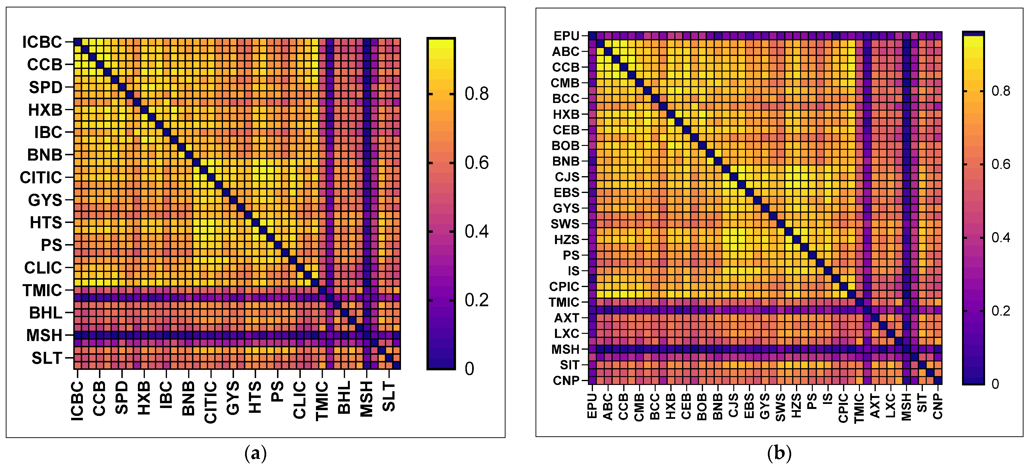
4.2. High-Dimensional Financial Network Connectedness Analysis

Constructing high-dimensional financial networks based on the elastic network shrinkage technology. Through this chapter, we can determine which financial institutions have a greater “to connectedness” and which have a greater “from connectedness”, and thus lay the foundation for the risk ripple-spreading network analysis.

Figure 2 below simultaneously present high-dimensional risk contagion networks during “the full sample”, “the stock market crash in China in 2015”, and “the COVID-19 pandemic in 2020”. Overall, the financial network structure and the risk contagion relationships between sectors show differentiated characteristics. The full sample analysis produces a measure of the average network during the sample period. In the full sample network, i.e., Figure 2a, some small- and medium-sized commercial banks such as HXB, CEB, SPD and BOB have a greater “to connectedness” and exhibit stronger risk spillover effects. Therefore, compared with the large state-owned commercial banks that are valued for being “too-big-to-fail”, we should guard against the occurrence of “black swan” events in small- and medium-sized commercial banks. Diversified financial institutions such as CNP, XLF, LXC, MCC and AJG have a greater “from connectedness” and show stronger vulnerability. Meanwhile, it can be seen from Figure 2c that some securities institutions such as CMS, IS, HTS and GFS show stronger risk spillover effects.

Based on the aforementioned network topology analysis method, we further discuss the risk cross-contagion relationship among the groups of sectors.

Table 2. Cross-sectoral network connectedness analysis of systemic financial risk **.

Panel A: Cross-sectoral network connectedness (2011–2023)
	$a$	$G{I}_{a\to b}$ (Group Influence)				IN-Mean	OUT-Mean	IFO-Mean	OTO-Mean
$b$		Banks	Securities	Insurance	Others
Banks		4.021	1.293	2.287	0.415	2.133	2.585	1.332	1.998
Securities		1.966	3.449	1.645	0.902	2.137	2.223	1.504	1.795
Insurance		2.831	1.812	2.625	0.900	2.036	1.885	1.848	1.763
Others *		1.198	2.280	1.358	1.917	1.715	0.933	1.612	0.739
Panel B: Cross-sectoral network connectedness (2015)
	$a$	$G{I}_{a\to b}$ (Group Influence)				IN-Mean	OUT-Mean	IFO-Mean	OTO-Mean
$b$		Banks	Securities	Insurance	Others
Banks		3.106	2.286	2.289	0.594	2.179	2.412	1.723	2.097
Securities		2.228	3.227	2.108	0.828	2.193	2.525	1.721	2.268
Insurance		2.445	2.524	2.625	0.846	2.112	2.131	1.938	2.053
Others *		1.617	1.994	1.761	2.065	1.847	1.001	1.791	0.756
Panel C: Cross-sectoral network connectedness (2020)
	$a$	$G{I}_{a\to b}$ (Group Influence)				IN-Mean	OUT-Mean	IFO-Mean	OTO-Mean
$b$		Banks	Securities	Insurance	Others
Banks		2.860	2.148	1.650	1.504	2.200	2.092	1.767	1.834
Securities		1.697	3.047	1.555	1.997	2.162	2.567	1.750	2.332
Insurance		2.453	2.007	3.522	1.334	2.122	1.772	1.932	1.650
Others *		1.350	2.840	1.746	2.447	2.102	1.846	1.979	1.612

* Notes: “Others” in Table 2 denotes the diversified financial industry. ** The cross-sectoral network connectedness indicators in Table 2 are calculated based on the aforementioned Equations (7)–(9).

below simultaneously present the cross-sectoral network connectedness results during “the full sample”, “the stock market crash in China in 2015” and “the COVID-19 pandemic in 2020”.

In observing Table 2, it can be found that the risk spillover effects within each group of sectors are higher than those between sectors, and the risk spillover effects between sectors show asymmetric characteristics. Specifically, both the banking and securities industries show significant net output effect of risk (OTO-Mean > IFO-Mean), which can have a significant impact on the financial market; the diversified financial industry always shows the net input effects of risk (OTO-Mean < IFO-Mean), which is more vulnerable to the risk shocks of financial market. In addition, during the full sample period, the banking industry has the highest network contagion connectedness with the highest values of $G{I}_{a\to b}$, OUT-mean and OTO-mean; however, during the period of major risk events, although network connectedness within sectors still dominates the system network, cross-sectoral network connectedness and risk spillover effects show a clear upward trend. Especially, the securities industry has a higher network contagion connectedness than the banking industry. Therefore, with the gradual maturity of China’s capital market, the financial regulatory authorities need to pay close attention to the capital flow and various leverage activities of securities institutions, and should strengthen the risk supervision of the securities industry in times especially during major risk events.

Further, we use the rolling time window technology to capture the dynamics of the financial network. To achieve a balance between trend spotting and sample size, the window size is chosen to be 240 days, or roughly 1 year. Figure 3 below shows the dynamic spillover index of systemic financial risk under the high-dimensional network model.

Overall, systemic financial risk in China from 2012 to 2023 is characterized by periodic cyclical fluctuations, and the aggregate network connectedness of the financial system increases significantly under internal and external risk shocks. The shaded areas of Figure 3 mark the intervals of obvious fluctuation, which correspond to various market extremes events such as “China’s Banking money shortage in 2013”, “the stock market crash in China in 2015”, “Sino-US trade friction in 2018” and “the COVID-19 pandemic in 2020”. Combined with the reality of economic operation in these periods, it can be found that systemic financial risk is in a phase of rising or local peak periods often accompanied by the outbreak of typical economic and financial events or external risk events. Therefore, the high-dimensional dynamic network model captures the risk characteristics of the financial system better and is consistent basically with the actual situation of the Chinese economic and financial system. Meanwhile, the findings above provide a pavement for the later analysis of the dynamic ripple-spreading paths of systemic financial risk.

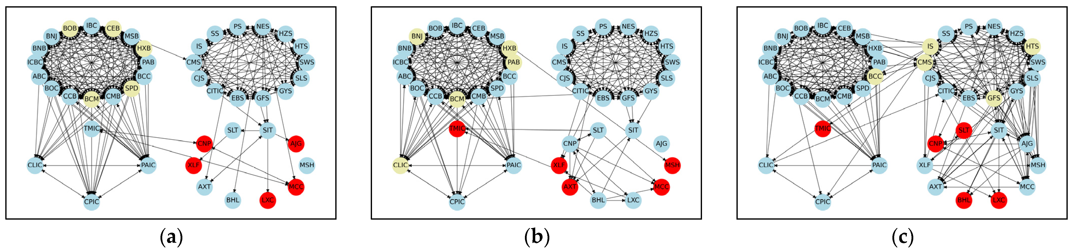
4.3. Ripple-Spreading Network Analysis of Systemic Risk Contagion

The above research shows that the network connectedness of the financial system increases significantly in the period of violent fluctuations in the financial market, policy shocks and the spread of external risks. Next, we will examine the dynamic ripple-spreading processes of systemic financial risk contagion under the impact of internal and external risks. However, how to use the findings of the aforementioned empirical studies to support the simulation design and make it more consistent with the financial risk contagion characteristics is the focus of this paper.

4.3.1. Parameter Specification for Risk Ripple-Spreading Network

Contagion sources selection. On the one hand, the financial system is exposed to internal shocks such as the bankruptcy of financial institutions and violent fluctuations in financial markets, etc. In the structure of China’s financial network, the banking sector occupies an important position, with its assets accounting for more than 80% of the overall proportion; thus, preventing systemic risk in the banking sector has become the core of maintaining financial stability. In general, large state-owned commercial banks show stability. The aforementioned studies especially have shown that some small- and medium-sized commercial banks exhibit stronger risk spillover connectedness compared to large state-owned commercial banks. Therefore, we select HXB as the source of internal contagion, which has the strongest risk spillover effect in the full-sample high-dimensional network. On the other hand, the financial system is simultaneously exposed to external shocks such as public health events, international financial market volatility, and policy uncertainty, etc. Existing studies show that “uncertainty” has become a new important driver of systemic financial risk [36,37]. Therefore, we select China’s economic policy uncertainty (EPU) [38] as a proxy variable for “uncertainty” to examine the risk ripple-spreading paths of the financial system in response to external shocks. The EPU index is constructed based on big data from news texts and covers a comprehensive dimension of “uncertainty” including not only economic and financial, but also regulatory and political uncertainty events. In particular, the EPU index takes its natural logarithmic form. EPU data from: http://www.policyuncertainty.com/ (accessed on 10 March 2023).

Initial energy value of contagion source: $E_0$. $E_0$ measures the magnitude of the systemic financial shock. To ensure sufficient network connectivity, the initial energy value of the contagion sources is set as follows:

$$e_{HXB}(t)=E_{HXB}=200\pi ; e_{EPU}(t)=E_{EPU}=200\pi$$

(16)

Amplifying factor: ${\alpha }_i$. ${\alpha }_i$ represents the contagion amplifying capability of the institution $i$. Since systemic financial risk is primarily driven by firm size [39], we argue that financial institutions with larger market capitalization have a stronger ability to amplify financial contagion. Thus, we use the market capitalization of the financial institutions to specify ${\alpha }_i$. For example, the average market capitalization of ICBC in the sample period is 16.358 × 100 billion yuan, so we set the amplifying factor ${\alpha }_{ICBC}=16.358$.

Connection threshold: ${\beta }_i$. ${\beta }_i$ reflects the resistance of financial institution $i$ to risk contagion. The calculation process of ${\beta }_i$ is similar to $X_{i\leftarrow j}^H$ in the spillover index method proposed by Diebold et al. [25]. Thus, we assume that financial institutions with larger spillover effects from other institutions are more vulnerable to financial contagion. Meanwhile, to solve the “dimensional curse” problem, we specify the parameter based on the above-mentioned high-dimensional risk spillover network.

Based on Equation (4), ${\beta }_i$ can be specified as follows:

$${\beta }_i=\frac{1}{{\displaystyle {\sum }_{j=1}^N{X}_{i\leftarrow j}^H}} , i\ne j$$

(17)

where $X_{i\leftarrow j}^H$ denotes the risk spillover effect of financial institution $j$ on $i$.

Spreading speed: $s_i$. $s_i$ affects the time required for ripple diffusion to form a stable network, but does not affect the final network topology. We assume that financial institutions with good stock liquidity will spread faster once they cause risk contagion. Thus, we use stock turnover rate to specify the parameters.

Market distance: $d_{ij}$. $d_{ij}$ represents the market distance financial institution $i$ and $j$, which is determined by the reciprocal of their volatility correlation coefficient.

Thus, $d_{ij}$ is specified as shown in Equation (18):

$$d_{ij}=\frac{1}{\left|co{r}_{ij}\right|}, if co{r}_{ij}\ne 0 ; d_{ij}=+\infty , if co{r}_{ij}=0$$

(18)

where $co{r}_{ij}$ is the correlation coefficient calculated based on history volatility data between financial institutions $i$ and $j$. In this paper, the higher the correlation between two financial institutions, the shorter the distance.

Table 3. Model parameters of risk ripple-spreading network *.

	ICBC	ABC	BOC	CCB	BCM	CMB	SPD	BCC	PAB	HXB	MSB
${\alpha }_i$	16.358	10.333	9.306	12.730	3.604	6.132	2.663	2.338	1.907	0.944	2.351
${\beta }_i$	1.101	1.098	1.089	1.087	1.083	1.083	1.082	1.091	1.094	1.082	1.092
$s_i$	0.065	0.190	0.093	0.961	0.326	0.364	0.466	0.147	0.784	0.510	0.478
	CEB	IBC	BOB	BNJ	BNB	CMS	CJS	CITIC	EBS	GFS	GYS
${\alpha }_i$	1.662	2.972	1.026	0.587	0.970	1.007	0.379	2.159	0.570	1.059	0.311
${\beta }_i$	1.085	1.088	1.091	1.092	1.107	1.072	1.077	1.068	1.092	1.082	1.089
$s_i$	0.497	0.636	0.463	0.812	0.716	0.601	1.109	1.385	1.127	1.051	1.300
	SLS	SWS	HTS	HZS	NES	PS	SS	IS	CLIC	CPIC	PAIC
${\alpha }_i$	0.308	0.310	1.261	1.094	0.204	0.220	0.225	0.442	6.528	2.381	8.046
${\beta }_i$	1.124	1.115	1.076	1.071	1.085	1.099	1.106	1.084	1.107	1.098	1.096
$s_i$	1.824	0.868	1.044	1.097	1.579	2.291	3.368	1.795	0.104	0.454	0.790
	TMIC	XLF	AXT	BHL	LXC	MCC	MSH	AJG	SIT	SLT	CNP
${\alpha }_i$	0.192	0.044	0.223	0.216	0.134	0.187	0.036	0.135	0.127	0.037	0.516
${\beta }_i$	1.291	2.031	1.198	1.206	1.241	1.259	2.124	1.402	1.133	1.261	1.314
$s_i$	1.226	2.760	1.433	1.116	1.454	2.298	2.060	1.603	1.854	2.812	0.977

* Note: The data in Table 3 are compiled by the authors based on the Equations (17) and (18). When the contagion source is EPU, we set ${\alpha }_{EPU}=0$, ${\beta }_{EPU}=+\infty$, and the propagation speed of EPU is taken as the average of all financial institutions.

below shows the parameters ${\alpha }_i$, ${\beta }_i$ and $d_{ij}$. Considering the market distances are specified by correlation, to save space, Figure 4 shows the heat map of correlation coefficients between financial institutions. It can be found that banks, securities and insurance have a higher correlation, i.e., shorter distance, while diversified financial institutions are relatively far from banks, securities and insurance.

4.3.2. Dynamic Ripple-Spreading Process of Systemic Risk under Internal Shocks

Based on the above simulation steps and network parameter setting guidelines, we simulate the dynamic ripple-spreading process of systemic financial risk contagion under internal and external shocks. Start the ripple-spreading procedure, record the instantaneous state and network topology of the risk ripple-spreading once every period Δt = 1 and select some representative instantaneous networks to study the dynamic risk contagion process.

Figure 5 below records the dynamic rippling-spreading process of systemic financial risks under the impact of HXB. On the whole, the contagion triggered by HXB first spreads within the banking industry, then spreads to the insurance and the securities industry and finally spreads to the diversified financial industry, thus triggering the cross-sectoral contagion. It can be found that financial contagion is more likely to occur between institutions in the same industry than between institutions across industries, which further confirms the findings of the aforementioned high-dimensional network model.

Specifically, Figure 5a–c shows risk contagion triggered directly by HXB. When t = 21, the contagion source HXB first triggers risk contagion within the banking industry and establishes directed connections with BOB, BCM, SPD and MSB, etc. As the risk ripple-spreading continues, all banking institutions and most insurance and securities institutions are directly affected by the impact of the contagion source HXB at t = 27, when the ripple effect of financial risk contagion first reaches the diversified financial industry (SIT). It indicates that banks are more closely networked with insurance and securities financial institutions and are more prone to financial contagion among them, while they are relatively distant from diversified financial institutions. Figure 5d–f shows that the risk contagion triggered by HXB continues to spread. At the same time, the risk cross-contagion occurs among financial institutions outside the wave source node HXB, and this cross-contagion first appears within the securities industry. For example, when t = 30, CITIC issues directed links to some securities institutions such as EBS, CJS, and HTS. When t = 32, the ripple effect of the securities industry begins to spread to other financial industries. These suggest that the securities industry assumes an intermediary role in the risk ripple network, receiving risk ripples from the banking sector while rapidly transmitting risk outward, and that the two-way risk contagion effect between the banking and securities industries plays an amplifier role in the evolution of systemic financial risk. Figure 5g–i show that the risk cross-contagion among financial institutions spreads widely and the networked contagion channels accelerate the evolution of systemic financial risk. When t = 48, all financial institutions are exposed to risk contagion, and complex and extensive network connections are established among financial institutions in all sectors.

To more clearly show the network characteristics of systemic financial risk ripple-spreading under HXB shocks,

Table 4. Statistical indicators of network nodes: HXB is set as contagion source (t = 48) *.

	ICBC	ABC	BOC	CCB	BCM	CMB	SPD	BCC	PAB	HXB	MSB
Out-degree	0	0	0	40	0	0	19	0	31	41	20
In-degree	30	30	31	30	32	31	30	32	29	31	30
	CEB	IBC	BOB	BNJ	BNB	CMS	CJS	CITIC	EBS	GFS	GYS
Out-degree	30	28	21	40	39	35	41	41	40	40	40
In-degree	30	30	31	31	30	30	31	31	27	27	27
	SLS	SWS	HTS	HZS	NES	PS	SS	IS	CLIC	CPIC	PAIC
Out-degree	41	40	41	41	41	42	42	42	0	0	40
In-degree	27	27	32	32	28	26	24	27	28	29	30
	TMIC	XLF	AXT	BHL	LXC	MCC	MSH	AJG	SIT	SLT	CNP
Out-degree	13	0	40	39	40	41	0	0	42	43	18
In-degree	25	5	27	24	26	24	1	13	26	25	25

* Note: The data in Table 4 are compiled by the authors based on the ripple-spreading network.

below reports the statistical indicators of the network’s out-degree and in-degree at t = 48. It can be found that the in-degree value of all banking institutions is above 30, while the out-degree values show different characteristics. Among them, large state-owned commercial banks such as ICBC, ABC, BOC and BCM play the role of financial stabilizer in the risk ripple-spreading network, and mainly accept the external risk without further amplifying the ripple effect (out-degree = 0). The out-degree value of joint-stock commercial banks such as HXB, PAB, MSB, CEB and IBC and city commercial banks such as BOB, BNJ and BNB are all above 20, indicating that small- and medium-sized commercial banks show strong risk ripple-spreading ability when facing shocks. Therefore, compared with the large state-owned commercial banks that are valued for being “too-big-to-fail”, we should guard against the occurrence of “black swan” events in small- and medium-sized banks. The out-degree value of securities financial institutions ranges from 35 to 42, and the in-degree value ranges from 24 to 32, indicating that securities institutions have strong risk linkage ability in the system network, which are not only easy to be stimulated by risk ripples, but also have a very strong ability to spread risk ripples outward. Additionally, the securities institutions mainly play a net spillover role in the ripple-spreading network (out-degree > in-degree). Finally, as the end node of the correlation network, the diversified financial industry engaged in financial-like business is vulnerable to systemic shocks, and its interaction with the securities industry may amplify the overall market volatility. Such institutions have low stock market value and high turnover rates, and it is recommended that the regulators guide rational investment, avoid the “herd effect” and curb speculative behavior.

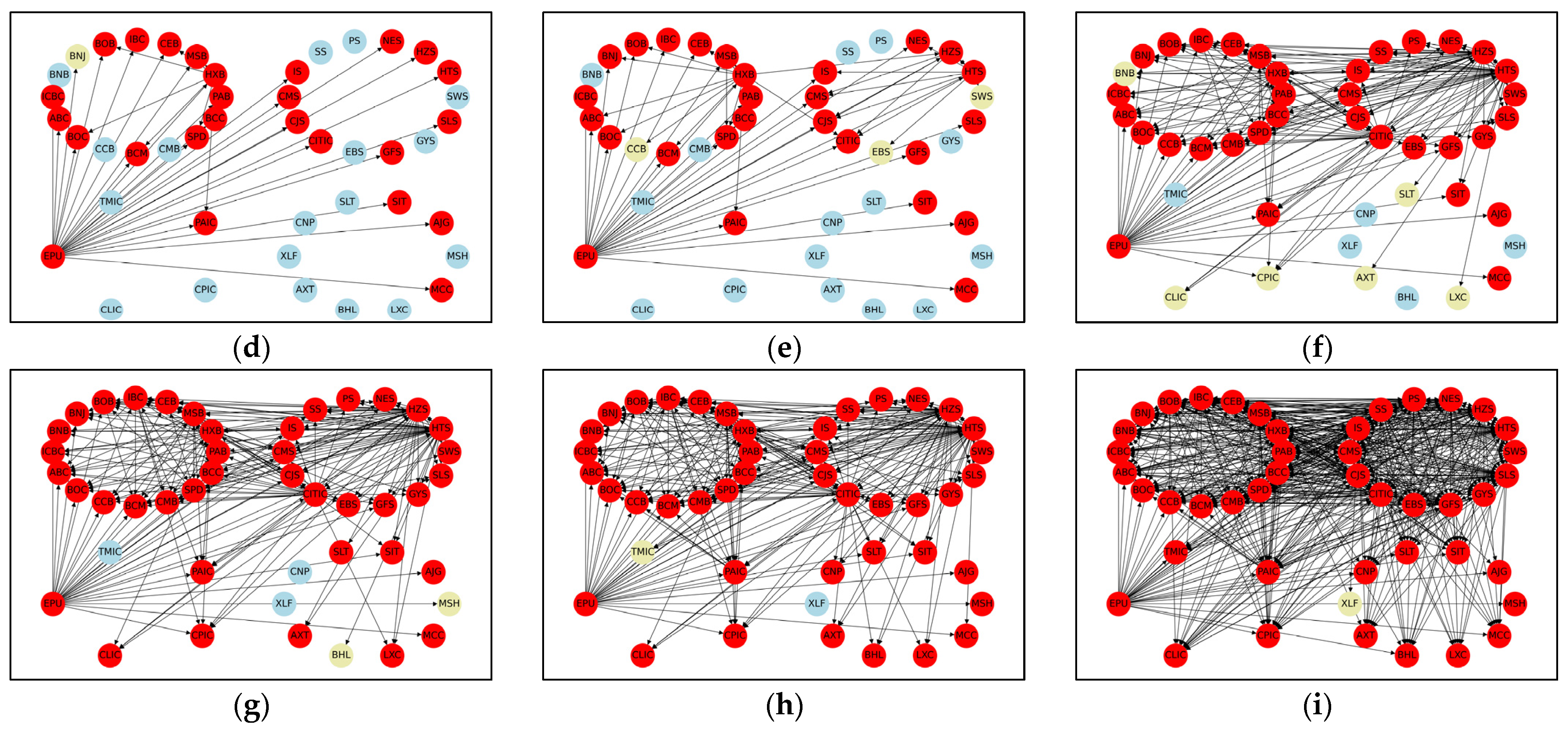
4.3.3. Dynamic Ripple-Spreading Process of Systemic Risk under External Shocks

Since the object of this study is financial institutions and EPU is the source of external contagion, EPU sends directed edges to financial institutions, but financial institutions do not send directed edges to EPU in the ripple-spreading network. Therefore, the connection threshold of EPU is set as ${\beta }_{EPU}=+\infty$; the risk amplification factor of EPU is set as ${\alpha }_{EPU}=0$. Additionally, the propagation speed of EPU is taken as the average of all financial institutions. Then, start the ripple-spreading procedure, record the instantaneous state and network topology of the risk ripple-spreading once every period Δt = 1 and select some representative instantaneous networks to study the dynamic risk contagion process.

Figure 6 below records the dynamic rippling-spreading process of systemic financial risks under the impact of EPU. On the whole, the contagion triggered by EPU first spreads to banks, and then to diversified financial institutions, securities and insurance institutions, successively, thus triggering the cross-sectoral networked contagion of systemic financial risks. Specifically, Figure 6a–c shows that four sectors are directly affected by EPU, and it can be seen that EPU has the most significant risk impact on the banking sector. When t = 40, almost all bank institutions are directly affected by EPU. The possible reason for this is that the banking sector, as a core component of China’s financial system, not only assumes the responsibility of serving the real economy, but also serves as an important transmission channel for the implementation effect of macro policies. Therefore, the banking sector is more profoundly and deeply affected by EPU shocks. In addition, it is worth noting that the diversified financial industry is affected before the insurance and securities industry when facing external shocks. Although the cross-sectoral risk spillover effect of diversified financial institutions is not so strong (see Table 2) and its scale is not as large as that of financial institutions such as banks and insurance, they are very vulnerable to external shocks. Figure 6d–i shows the process of risk cross-contagion among financial institutions triggered by EPU. It can be found that cross-sectoral risk contagion among financial institutions is gradually penetrating, the connections within the financial system are becoming more complex and the network density is gradually increasing. When t = 52, all financial institutions are affected by EPU. The number of network connections at t = 52 is significantly higher than that at t = 48, which indicates that the risk contagion among financial institutions is very rapid.

To more clearly show the network characteristics of systemic financial risk ripple-spreading under EPU shocks,

Table 5. Statistical indicators of network nodes: EPU is set as contagion source (t = 52) *.

	ICBC	ABC	BOC	CCB	BCM	CMB	SPD	BCC	PAB	HXB	MSB
Out-degree	0	0	0	0	0	0	31	0	15	36	33
In-degree	16	18	17	18	18	16	17	17	15	17	17
	CEB	IBC	BOB	BNJ	BNB	CMS	CJS	CITIC	EBS	GFS	GYS
Out-degree	0	29	28	0	0	0	28	40	0	34	0
In-degree	18	16	16	17	17	18	16	17	16	16	16
	SLS	SWS	HTS	HZS	NES	PS	SS	IS	CLIC	CPIC	PAIC
Out-degree	41	0	40	40	41	39	40	42	0	0	31
In-degree	15	13	17	16	16	16	12	16	16	17	17
	TMIC	XLF	AXT	BHL	LXC	MCC	MSH	AJG	SIT	SLT	CNP
Out-degree	0	0	0	0	0	0	0	0	0	0	0
In-degree	8	1	9	11	8	9	1	4	14	9	10

* Note: The data in Table 5 are compiled by the authors based on the ripple-spreading network. At this moment (t = 52), the out-degree value of EPU is 36; the in-degree value of EPU is 0.

below reports the statistical indicators of the network’s out-degree and in-degree at t = 52. Although the external shock changes the risk contagion paths of the financial network, as the risk ripples continue, the final network topology shows similar characteristics. For example, large state-owned commercial banks such as ICBC, ABC, BOC, CCB and BCM are still the main bearers of risk ripples (Out-degree = 0). Small- and medium-sized commercial banks such as HXB, MSB, SPD and IBC still show strong risk ripple-spreading ability. (The out-degree is about 30.) It is worth noting that the number of network connections at t = 52 is 622, which is lower than the number of network connections under internal shocks at t = 48, indicating that systemic risk spread faster under the internal shock and wider under the external shock. However, the risk ripple-spreading process is not yet sufficient at this moment (t = 52). Figure 7 below further gives the average network indicators for each sector with an upper time limit of t = 500. It can be found that the out-degree values of the four financial sectors show different characteristics, while the in-degree values show similar characteristics. The securities industry especially also shows strong risk linkage ability and occupies a dominant position in the process of risk ripple-spreading. As the risk ripple-spreading process continues, the networked contagion channels within the financial system will accelerate the evolution of systemic financial risk. Therefore, in the face of external shocks, the regulatory authorities should find the right time to cut off the risk contagion paths before the networked contagion channels are fully established, which can effectively prevent the spread of risks.

5. Conclusions

In this paper, we examine the contagion mechanism of systemic financial risk in China based on a dynamic network perspective. First, we construct a high-dimensional financial network model to extract connectedness information related to the spillover effects of systemic risk. On this basis, the ripple-spreading network model is introduced and improved to simulate the dynamic contagion paths of systemic financial risk under given shocks. This study provides a new perspective to prevent the risk of contagion in the financial sector. Compared with the existing correlation networks, causal networks and spillover networks, the ripple-spreading network can better describe the spatial and temporal phenomena of financial contagion and can reveal how financial contagion spreading from the contagion source to the whole financial system in the form of dynamic networks. According to the dynamic and intuitive paths, it is convenient to analyze which financial institutions are first infected with financial contagion and which are later. This is crucial for preventing financial contagion. In addition, the established hypotheses of the ripple-spreading network are research-based results that refer to the performed spillover index calculations and contribute to the elimination of the risk of financial contagion.

The empirical results show that financial contagion is more likely to occur between financial institutions within the same industry. As the risk ripples continue to spread, cross-sectoral risk contagion connectedness increases rapidly. The risk ripple-spreading process exhibit some differences under different shocks. The distinctive feature is that risk ripples spread faster under internal shocks and wider under external shocks. In the face of HXB internal shocks, the risk ripple first spreads within the same industry, then spreads to the insurance and securities industries, and finally spreads to the diversified financial institutions. In the face of EPU external shocks, the banking industry is the first to be directly affected, followed by the diversified financial industry, the insurance industry and the securities industry, thus triggering the cross-sectoral contagion. Compared with the insurance and securities industry, the diversified financial industry is more vulnerable to the external environment, although its scale is relatively small. In addition, we also find some common characteristics. In addition, when facing internal and external financial shocks, some small- and medium-sized commercial banks show stronger ripple-spreading abilities than the large state-owned commercial banks in the process of risk contagion. The securities industry is more responsive to risk shock than the banking industry, and shows the most active risk linkage characteristics in the risk ripple-spreading network. The securities industry especially is the intermediary layer of the ripple-spreading network and plays an amplifier role in the contagion and evolution of systemic financial risk.

The conclusion of this paper has certain guiding significance for the supervision practice of systemic financial risk. Firstly, network correlation is an important component of systemic financial risk. Real-time monitoring of the dynamic evolution characteristics of the financial network structure can help policymakers to capture the changes in risk in time, and provide references for macro-prudential management from the perspective of the global network. Secondly, the RSNM model can intuitively present the dynamic contagion paths of systemic financial risk triggered by contagion sources in the form of dynamic networks, thus providing an intuitive reference for the formulation of financial risk prevention strategies. At the same time, setting different contagion sources to simulate the risk ripple-spreading paths can also provide strong evidence for the early warning and prevention of major risks. Finally, systemic financial risk regulation should focus not only on large financial institutions, but also on financial institutions with strong ripple effects. The securities industry is the intermediary layer of the ripple-spreading network. During major risk events, isolating risk intermediary nodes can effectively cut off the paths of risk contagion and mitigate the impact on the whole financial system.

References

1. Yadav, M.P.; Rao, A.; Abedin, M.Z.; Tabassum, S.; Lucey, B. The domino effect: Analyzing the impact of Silicon Valley Bank’s fall on top equity indices around the world. Financ. Res. Lett. 2023. [Google Scholar] [CrossRef]
2. Granger, C.W.J. Can We Improve the Perceived Quality of Economic Forecasts? J. Appl. Econom. 1996, 11, 455–473. [Google Scholar] [CrossRef]
3. Bostanci, G.; Yilmaz, K. How connected is the global sovereign credit risk network? J. Bank. Financ. 2020, 113, 105761. [Google Scholar] [CrossRef]
4. Betz, F.; Hautsch, N.; Peltonen, T.A.; Schienle, M. Systemic risk spillovers in the European banking and sovereign network. J. Financ. Stab. 2016, 25, 206–224. [Google Scholar] [CrossRef]
5. Gross, C.; Siklos, P.L. Analyzing credit risk transmission to the nonfinancial sector in Europe: A network approach. J. Appl. Econ. 2020, 35, 61–81. [Google Scholar] [CrossRef]
6. Hull, J.C. Risk Management and Financial Institutions; Wiley Finance Series: Hoboken, NJ, USA, 2015. [Google Scholar]
7. Xu, F. Modeling the Paths of China’s Systemic Financial Risk Contagion: A Ripple Network Perspective Analysis. Comput. Econ. 2022, 1–27. [Google Scholar] [CrossRef]
8. Su, Z.; Xu, F. Dynamic identification of systemically important financial markets in the spread of contagion: A ripple network based collective spillover effect approach. J. Multinatl. Financ. Manag. 2021, 60, 100681. [Google Scholar] [CrossRef]
9. Hu, X.-B.; Wang, M.; Leeson, M.; Hines, E.L.; Di Paolo, E. Deterministic ripple-spreading model for complex networks. Phys. Rev. E 2011, 83, 046123. [Google Scholar] [CrossRef]
10. Hu, X.-B.; Wang, M.; Leeson, M.S. Ripple-Spreading Network Model Optimization by Genetic Algorithm. Math. Probl. Eng. 2013, 2013, 176206. [Google Scholar] [CrossRef]
11. Jie, K.-W.; Liu, S.-Y.; Sun, X.-J.; Xu, Y.-C. A dynamic ripple-spreading algorithm for solving mean–variance of shortest path model in uncertain random networks. Chaos Solitons Fractals 2023, 167, 113081. [Google Scholar] [CrossRef]
12. Soramäki, K.; Bech, M.L.; Arnold, J.; Glass, R.J.; Beyeler, W.E. The topology of interbank payment flows. Phys. A Stat. Mech. Its Appl. 2007, 379, 317–333. [Google Scholar] [CrossRef]
13. Borges, M.R.; Ulica, L.; Gubareva, M. Systemic risk in the Angolan interbank payment system–A network approach. Appl. Econ. 2020, 52, 4900–4912. [Google Scholar] [CrossRef]
14. Mistrulli, P.E. Assessing financial contagion in the interbank market: Maximum entropy versus observed interbank lending patterns. J. Bank. Financ. 2011, 35, 1114–1127. [Google Scholar] [CrossRef]
15. Giudici, P.; Sarlin, P.; Spelta, A. The interconnected nature of financial systems: Direct and common exposures. J. Bank. Financ. 2020, 112, 105149. [Google Scholar] [CrossRef]
16. Sui, P.; Tanna, S.; Zhou, D. Financial contagion in a core-periphery interbank network. Eur. J. Financ. 2019, 26, 691–710. [Google Scholar] [CrossRef]
17. Chiba, A. Financial Contagion in Core–Periphery Networks and Real Economy. Comput. Econ. 2020, 55, 779–800. [Google Scholar] [CrossRef]
18. Benoit, S.; Colliard, J.-E.; Hurlin, C.; Pérignon, C. Where the Risks Lie: A Survey on Systemic Risk. Rev. Financ. 2017, 21, 109–152. [Google Scholar] [CrossRef]
19. Mao, X.; Wei, P.; Ren, X. Climate risk and financial systems: A nonlinear network connectedness analysis. J. Environ. Manag. 2023, 340, 117878. [Google Scholar] [CrossRef] [PubMed]
20. Pereira, E.J.D.A.L.; Ferreira, P.J.S.; da Silva, M.F.; Miranda, J.G.V.; Pereira, H.B. Multiscale network for 20 stock markets using DCCA. Phys. A Stat. Mech. Its Appl. 2019, 529, 121542. [Google Scholar] [CrossRef]
21. Aslam, F.; Mohmand, Y.T.; Ferreira, P.; Memon, B.A.; Khan, M.; Khan, M. Network analysis of global stock markets at the beginning of the coronavirus disease (COVID-19) outbreak. Borsa Istanb. Rev. 2020, 20, S49–S61. [Google Scholar] [CrossRef]
22. Billio, M.; Getmansky, M.; Lo, A.W.; Pelizzon, L. Econometric measures of connectedness and systemic risk in the finance and insurance sectors. J. Financ. Econ. 2012, 104, 535–559. [Google Scholar] [CrossRef]
23. Brunetti, C.; Harris, J.H.; Mankad, S.; Michailidis, G. Interconnectedness in the interbank market. J. Financ. Econ. 2019, 133, 520–538. [Google Scholar] [CrossRef]
24. Bu, H.; Tang, W.; Wu, J. Time-varying comovement and changes of comovement structure in the Chinese stock market: A causal network method. Econ. Model. 2019, 81, 181–204. [Google Scholar] [CrossRef]
25. Diebold, F.X.; Yılmaz, K. On the network topology of variance decompositions: Measuring the connectedness of financial firms. J. Econ. 2014, 182, 119–134. [Google Scholar] [CrossRef]
26. Nguyen, L.X.D.; Mateut, S.; Chevapatrakul, T. Business-linkage volatility spillovers between US industries. J. Bank. Financ. 2020, 111. [Google Scholar] [CrossRef]
27. Härdle, W.K.; Wang, W.; Yu, L. TENET: Tail-Event driven NETwork risk. J. Econ. 2016, 192, 499–513. [Google Scholar] [CrossRef]
28. Chen, H.; Sun, T. Tail Risk Networks of Insurers around the Globe: An Empirical Examination of Systemic Risk for G-SIIs vs Non-G-SIIs. J. Risk Insur. 2020, 87, 285–318. [Google Scholar] [CrossRef]
29. Abduraimova, K. Contagion and tail risk in complex financial networks. J. Bank. Financ. 2022, 143, 106560. [Google Scholar] [CrossRef]
30. Wang, G.-J.; Chen, Y.-Y.; Si, H.-B.; Xie, C.; Chevallier, J. Multilayer information spillover networks analysis of China’s financial institutions based on variance decompositions. Int. Rev. Econ. Financ. 2021, 73, 325–347. [Google Scholar] [CrossRef]
31. Ouyang, Z.; Zhou, X. Multilayer networks in the frequency domain: Measuring extreme risk connectedness of Chinese financial institutions. Res. Int. Bus. Financ. 2023, 65, 101944. [Google Scholar] [CrossRef]
32. Chan, L.S.H.; Chu, A.M.Y.; So, M.K.P. A moving-window bayesian network model for assessing systemic risk in financial markets. PLoS ONE 2023, 18, e0279888. [Google Scholar] [CrossRef] [PubMed]
33. Jiang, C.; Sun, Q.; Ye, T.; Wang, Q. Identification of systemically important financial institutions in a multiplex financial network: A multi-attribute decision-based approach. Phys. A Stat. Mech. Its Appl. 2023, 611, 128446. [Google Scholar] [CrossRef]
34. Demirer, M.; Diebold, F.X.; Liu, L.; Yilmaz, K. Estimating global bank network connectedness. J. Appl. Econ. 2018, 33, 1–15. [Google Scholar] [CrossRef]
35. Brownlees, C.; Hans, C.; Nualart, E. Bank credit risk networks: Evidence from the Eurozone. J. Monet. Econ. 2021, 117, 585–599. [Google Scholar] [CrossRef]
36. Dicks, D.L.; Fulghieri, P. Uncertainty Aversion and Systemic Risk. J. Political Econ. 2019, 127, 1118–1155. [Google Scholar] [CrossRef]
37. Wu, J.; Yao, Y.; Chen, M.; Jeon, B.N. Economic uncertainty and bank risk: Evidence from emerging economies. J. Int. Financ. Mark. Inst. Money 2020, 68, 101242. [Google Scholar] [CrossRef]
38. Baker, S.R.; Bloom, N.; Davis, S.J. Measuring Economic Policy Uncertainty. Q. J. Econ. 2016, 131, 1593–1636. [Google Scholar] [CrossRef]
39. Varotto, S.; Zhao, L. Systemic risk and bank size. J. Int. Money Financ. 2018, 82, 45–70. [Google Scholar] [CrossRef]
Figure 1. The basic idea of the semi-deterministic ripple-spreading network model. Note: Figure 1 is plotted by the authors on the basis of Hu et al. [9].
Mathematics 11 02267 g001
Figure 2. High-dimensional network connectedness for systemic risk (20% of the edges visible). Notes: (1) In each subgraph, the four regions represent banks, securities, insurance and diversified financial institutions, respectively; (2) the yellow and red nodes indicate the top five financial institutions in terms of “to connectedness” and “from connectedness”, respectively. (3) The network diagrams in Figure 2 are calculated and plotted based on the aforementioned Equation (4). (a) network connectedness: 2011–2023; (b) network connectedness: 2015; (c) network connectedness: 2020.
Mathematics 11 02267 g002
Figure 3. Aggregate connectedness index based on the high-dimensional risk contagion network. Note: The connectedness index in Figure 3 is calculated based on the Equation (6).
Mathematics 11 02267 g003
Figure 4. The heat map of correlation coefficients between financial institutions. (a) Shows the correlation coefficient matrix between financial institutions. (b) Shows the correlation coefficient matrix between EPU and financial institutions.
Mathematics 11 02267 g004
Figure 5. The ripple-spreading process: HXB is set as contagion source. Notes: (1) Each subgraph represents the instantaneous ripple network at a certain moment. (2) The four regions of each subgraph represent banks, securities, insurance and diversified financial institutions, respectively; (3) The blue nodes represent normal financial institutions that are not at risk of infection at the current time; yellow nodes indicate financial institutions that are not at risk of infection before the current moment, but are infected at the current moment; red nodes represent financial institutions that were infected before the current time. (a) Current time: t = 21, links: 7; (b) Current time: t = 25, links: 27; (c) Current time: t = 27, links: 31; (d) Current time: t = 30, links: 41; (e) Current time: t = 32, links: 106; (f) Current time: t = 34, links: 189; (g) Current time: t = 38, links: 534; (h) Current time: t = 42, links: 665; (i) Current time: t = 48, links: 1192.
Mathematics 11 02267 g005
Figure 6. The ripple-spreading process: EPU is set as contagion source. (Notes see Figure 5). (a) Current time: t = 23, links: 6; (b) Current time: t = 34, links: 18; (c) Current time: t = 40, links: 25; (d) Current time: t = 42, links: 33; (e) Current time: t = 43, links: 53; (f) Current time: t = 45, links: 166; (g) Current time: t = 46, links: 200; (h) Current time: t = 48, links: 257; (i) Current time: t = 52, links: 622.
Mathematics 11 02267 g006aMathematics 11 02267 g006b
Figure 7. Contagion network indicators of the ripple-spreading process under EPU shocks. Notes: Figure 7 is calculated and plotted based on the ripple-spreading process; “Others” denotes the diversified financial industry. (a) Average out-degree network indicators for the four financial sectors. (b) Average In-degree network indicators for the four financial sectors.
Mathematics 11 02267 g007