Abstract
This article explores complex-valued inertial neural networks (CVINNs) with distributed delays (DDs). By constructing two new feedback controllers, some novel results on fixed-time stabilization (FTS) and preassigned-time stabilization (PTS) of CVINNs are established. Unlike most of the previous works, FTS and PTS obtained here are explored without dividing the original complex-valued system into two separate real valued subsystems. Eventually, to verify the effectiveness and reliability of the results of this article, we provide several numerical examples. The FTS and PTS of CVINNs are successfully implemented at T = 6, 5.5, and 5, and the settling time is not affected by system parameters and initial values.
Keywords:
complex-valued neural networks; inertial terms; distributed delays; fixed-time stabilization; preassigned-time stabilization MSC:
93D05; 93D15
1. Introduction
Neural networks (NNs) have wide-ranging applications in signal processing, combinatorial optimisation, automatic control, and deep learning, which have received substantial attention in the last few decades. During the applications of NNs, of which dynamic behaviours are the key points. Among them, stabilization is the important one that has a wide range of applications in bioengineering, information processing, and other fields. As is well known, the settling time (ST) of finite-time is linked to the system’s initial conditions. Furthermore, a well-known fact is that the initial conditions of NNs are difficult to obtain in some cases. Therefore, the results of finite-time are conservative. In 2012, Polyakov [1] proposed the fixed-time theory, in which the estimation of the ST is independent of the initial state. In comparison to finite time stabilization, fixed-time stabilization (FTS) has better prospects for application and have come to be the focus of scientists and researchers. In [2], Liu and Zhang studied the FTS of fuzzy NNs by means of the theory of differential inclusion. In [3], the authors investigated the FTS problems for delayed memristive neural networks. In [4], Liu et al. have researched FTS of fuzzy inertial neural networks. However, FTS also has its disadvantages, of which ST is fixed and cannot be adjusted to meet some engineering applications. Fortunately, ST of preassigned-time stabilization (PTS) and synchronization discussed in [5,6] can be adjusted according to practical need, which has more meaningful in practical engineering applications.
Babcock and Westervelt first presented the concept of inertial neural networks (INNs) in 1986 by introducing inductance into neural circuits [7]. INNs are usually described by second-order differential equations. Compared with the traditional first-order NNs, INNs show more complex dynamic characteristics [8], such as instability, bifurcation, chaos, etc., and INNs helps to realize a chaotic search of memory in the application [9]. At the same time, adding inductors into NNs has broad biological background, which can simulate the membrane characteristics of the protruding pigeon vestibular hair cells of squid through inductance [10]. INNs have important applications in information processing; therefore, studies about the dynamics and control of INNs is of great importance. In [11,12,13,14], the theoretical results of global exponential stability, finite time stability, FTS, and preassigned-time synchronization (PTS) for INNs were obtained by employing the method of inserting intermediate variables and designing suitable controllers. Refs. [11,12,15] provide the application of INNs in the production of pseudo-random numbers and image encryption. In 2019, refs. [16,17] research the stability of the INNs by variable replacement. Many academics have conducted in-depth research on INNs and achieved some good theoretical results because INNs can solve many practical problems. This encourages us to further study INNs.
At the same time, because the limitations of physical components, which lead to the information transferring of NNs have always time delays [18]. Time delay can have an influence on the stability of NNs, which often leads to unstable oscillations and chaos [19,20]. Several classes of delay, such as constant delay, time-varying delay and distributed delay (DDs) have been, respectively, studied in relevant papers [21,22,23,24]. In [25,26], the authors discussed the passivity of fractional order NNs and quaternions NNs with time-varying delays, respectively. The stability of NNs with time-varying delays was investigated and some effective conditions were obtained in the work by Chen et al. [27]. Li et al. [28] studied the finite-time synchronization of quaternion-valued NNs with mixed-delays and some effective synchronisation criteria are reached by constructing novel feedback strategies. However, most of the above results are discussed in finite-time, and the NNs are also considered without inertial terms. So, the investigation of FTS and PTS of INNs with DDs are meaningful and necessary.
On the other hand, the above discussions are all based on real-valued NNs, in fact, in some practical applications, there often exist complex signals, such as information, flow of speech synthesis, and optoelectronics [29,30,31,32,33]. Compared to real-valued NNs, complex-valued neural networks (CVNNs) have superior characteristics, such as faster computing speed, greater processing capacity, and can solve problems that the real-valued system cannot, such as the well-known XOR problem [34]. As we know, the research method of complex-valued system is different from a real-valued system. In most cases, the complex-valued systems are split into two systems with real and imaginary parts, then real-valued approach can be used. There are a lot of literatures, e.g., see [35,36,37,38,39,40,41,42], which use separation method to study asymptotic synchronization, exponential synchronization and FTS. Although the separation approach is feasible, two issues will arise, firstly, dimension of the systems will increase after decomposition, and the processes of theoretical analysis will become more cumbersome. Secondly, it is difficult to decompose complex valued systems into corresponding real part systems and imaginary part systems in practical applications. Hence, it is profoundly meaningful to deal with complex-valued systems with a non-separation approach.
Based on the above discussions, to ensure that the results of complex-valued systems are more rigorous and scientific, in this article, without dividing complex-valued INNs into the real and imaginary parts, some effective results are derived to realize the FTS and PTS for complex-valued inertial neural networks (CVINNs) with DDs. The following contents are the major contributions of this article:
1. Unlike the NNs considered in previous works, refs. [43,44,45,46,47,48] only defined in the real number field, ref. [5] without inertial term, refs. [2,3,9,13] do not consider the DDs. The model of this article is with inertial term, DDs and defined in complex number domain, which is more general and meaningful.
2. In contrast to split the complex system into real and imaginary parts [35,36,37,38,39,40,41,42], this article proposes a suitable control strategy to implement FTS of CIVNNs with DDs by using a non-separation approach and some new criteria are obtained.
3. PTS were not investigated in [2,3,9,13,47,48]. By using a non-separation approach, we obtain some new results on PTS of CIVNNs with DDs, and the ST of PTS do not depend on any initial values and parameters of the CIVNNs.
Symbol Description: In this article, stand for set of real numbers, set of complex numbers and n-dimensional complex-valued vectors, respectively. In addition, m represents the imaginary unit, for any , the conjugate expression of is , , . In addition, the represents the sign function of any .
2. Preliminaries
The system can be described by
and the initial values are
where , n represents number of neurons, is the state of the neuron at time t; ; depict the neuron connection weights. denote the activation function. is delays, is distributed delays. Furthermore, , .
When the parameters of system (1) are inappropriate, the system (1) is unstable. To stabilize system (1), we build a controller and add it to the system (1) to obtain the system (3).
where is the control, which is given later.
Hypothesis 1.
For each , there are real numbers , such that for any ,
To further analyse the dynamical behaviour of the system (3), we give an intermediate variable , where are suitable constant. So, the system (3) was rewritten as
where , .
Definition 1
([6]). If for , , and is positive and irrelevant of the initial value of (4), one has , , then, system (4) implements FTS at .
Definition 2
([49]). If system (4) is FTS, for a predefined constant , ST , then, system (4) is called the PTS.
Lemma 1
([50]). For System (4), if is a radial unbounded function, the following inequality stands
where and , the system can achieve FTS, and the ST is estimated by
Lemma 2
([6]). For System (4), if is a radial unbounded function, the following inequality holds
where and the system can achieve PTS within prespecified time , and
Lemma 3
([51]). Let and one has
Lemma 4
([52]). For any , and any measurable selection , in which
The formula below is correct.
3. Main Results
In this part, we analyse the FTS and PTS of system (4) via novel control strategy.
3.1. FTS of System (4)
The system (4) can achieve FTS through the following control strategy:
where for , , and the framework of above designed controller is given in Figure 1.
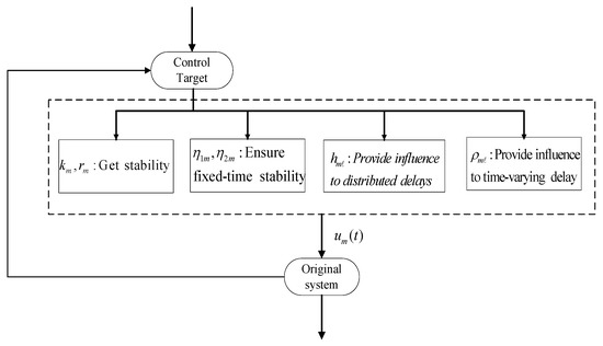
Figure 1.
Framework of designed controller.
Theorem 1.
Under Hypothesis 1, and the following inequality holds
then, the system (4) can achieve FTS, and the ST is
where ; ; ; .
Proof.
When , because the controller (5) is discontinuous, there is
By virtue of the measurable selection theorem, and because , such that
Now, we build the Lyapunov function as follows:
We calculate the derivative of along the solution of system (4), then, one has
□
According to the properties of norm of complex-valued number and Assumption 1,
Similar to above:
If the results of (12)–(14) are combined, then (11) is equivalent to:
Among,
According to Lemma 3, we can obtain
Similarly,
According to (17) and (18),
Therefore,
where ; ; .
Remark 1.
Construct simple Lyapunov function is important in discussing the FTS and PTS of NNs. Because the NNs in this article are complex-valued and Lyapunov function request positive definite, so, Lyapunov function with 2-norm are considered in our discussion.
Remark 2.
In the existing literature [2,5,53], although fixed-time synchronization or stabilization of NNs have been discussed. However, [53] ignored the DDs, [5] discussed the NNs only with first-order, and [2] only discussed the FTS in the real number domain. Therefore, the results obtained in this article are more general and extended the previous works.
3.2. PST of System (4)
The system (4) can achieve PTS through the following control strategy:
where , .
Theorem 2.
Under Hypothesis 1, the following inequality holds
the system (4) can achieve preassigned-time, and the preassigned-time is .
Proof.
Now, we build the Lyapunov functional as follows:
We calculate the derivative of along the solution of system (4), similar to the proof of Theorem 1, we obtain
where , ; .
□
Remark 3.
Here, we let and , which is better to ensure stability and achieve PTS of such CVINNs.
Remark 4.
Unlike [2,54,55,56], only considered finite/fixed-time results in the real number field, the PTS of INNs with complex-valued, and the DDs are studied; the results of this article further enrich the dynamics behaviours of NNs.
Remark 5.

In order to show the advantages of this article, some comparisons between the related previous works and this article is shown in Table 1:
Table 1.
The comparisons between the related previous works and this paper.
4. Numerical Example
To demonstrate the effectiveness of the FTS and PTS results, the relevant simulations and applications are as follows.
Example 1.
We consider the below reduced-order CVINNs with DDs.
where , , , ; , ; , , is control input.
The initial value are .
The dynamic behaviour of model (25) without controller is as shown in the Figure 2 and Figure 3. Obviously, the system (25) is unstable. We therefore design a controller to stabilise the system as shown.
In System (25), a continuous function satisfies Assumption 1 and . We know from straightforward computations that the conditions of Theorem 1 are all satisfied. We design the gain of the controller (26) as , . Meanwhile, the values of and here are as follows:

Figure 2.
The phase and states trajectories of real part of CVINNs (25) with , m = 1, 2.
Figure 2.
The phase and states trajectories of real part of CVINNs (25) with , m = 1, 2.


Figure 3.
The phase and states trajectories of the image part of CVINNs (25) with , m = 1, 2.
Figure 3.
The phase and states trajectories of the image part of CVINNs (25) with , m = 1, 2.

CVINN with DDs (25) is stable in fixed-time under control (26) which are shown in Figure 4. Furthermore, the setting time of the system (25) is . In the same way, we change the parameters to satisfy the requirement of Theorem 2. Set and 5, respectively. From Figure 5, Figure 6 and Figure 7, we can see that the system (25) reaches stabilization at 6, 5.5, and 5, respectively.
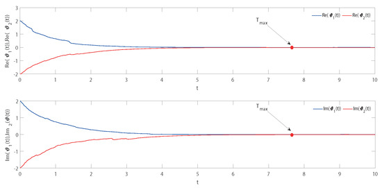
Figure 4.
The states trajectories of CVINNs with DDs (25) with control input (26).
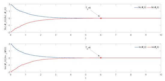
Figure 5.
The states trajectories of CVINNs with DDs (25) with control input (21).
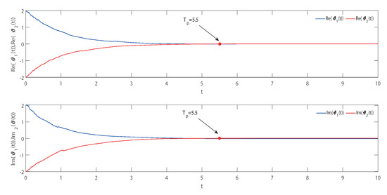
Figure 6.
The states trajectories of CVINNs with DDs (25) with control input (21).
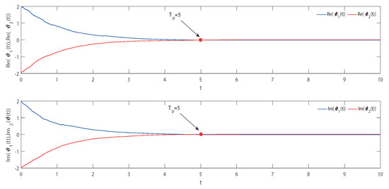
Figure 7.
The states trajectories of CVINNs with DDs (25) with control input (21).
By using results of FTS given above, the PRNG is obtained, which is represented in Figure 8. Allow to be the original transmitted signal as shown in Figure 9. Then obtain the encrypted signal, as illustrated in Figure 10. Due to the unstable nature of CVINNs with DDs, there is an enormous difference between encrypted signal created by PRNG and original signal.
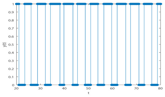
Figure 8.
The states PRNG obtained from CVINNs with DDs.
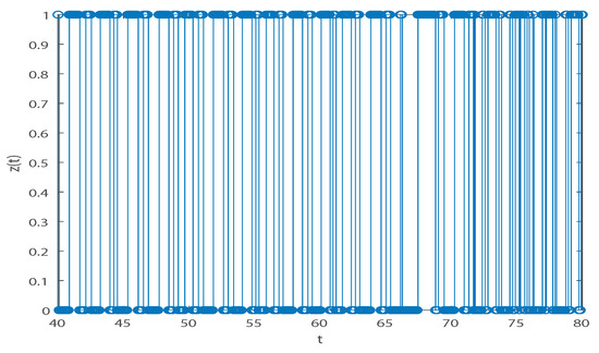
Figure 9.
Original signals.
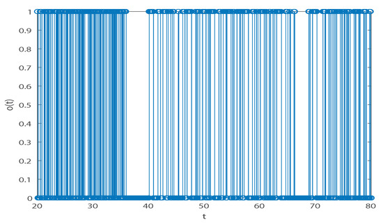
Figure 10.
Encrypted signals.
5. Conclusions
In this article, we provide some sufficient conditions to obtain the FTS and PTS of CVINNs with DDs. In contrast to previous studies, we study the dynamic behaviour of CVINNs by using the non-separation approach, which not only reduces the computational complexity but also reduces the inconvenience. Finally, we provide numerical examples for the FTS and PTS to verify the effectiveness of the obtained results, and an application of CVINNs with DDs in pseudorandom number generation is provided. Our future research directions include (1) extending the research results to CVINNs with state-dependent switching; and (2) investigating the dynamic behaviour of CVINNs by using event-triggered control and non-reduced order approach.
Author Contributions
Y.Y.: Writing and editing—original draft, software; G.Z.: Conceptualization, methodology, writing—review and and Supervision; Y.L.: Writing—review. All authors have read and agreed to the published version of the manuscript.
Funding
This work is supported by the National Science Foundation of China Nos. 61976228 and 62076106.
Data Availability Statement
Not applicable.
Conflicts of Interest
The authors declare no conflict of interest.
References
- Polyakov, A. Nonlinear feedback design for fixed-time stabilization of linear control systems. IEEE Trans. Autom. Control 2011, 57, 2106–2110. [Google Scholar] [CrossRef]
- Liu, Y.; Zhang, G.; Hu, J. Fixed-time stabilization and synchronization for fuzzy inertial neural networks with bounded distributed delays and discontinuous activation functions. Neurocomputing 2022, 495, 86–96. [Google Scholar] [CrossRef]
- Li, H.; Hu, C.; Zhang, G.; Hu, J.; Wang, L. Fixed-/Preassigned-time stabilization of delayed memristive neural networks. Inf. Sci. 2022, 610, 624–636. [Google Scholar] [CrossRef]
- Liu, J.; Shu, L.; Chen, Q.; Zhong, S. Fixed-time synchronization criteria of fuzzy inertial neural networks via Lyapunov functions with indefinite derivatives and its application to image encryption. Fuzzy Sets Syst. 2023, 459, 22–42. [Google Scholar] [CrossRef]
- Gan, Q.; Li, L.; Yang, J.; Qin, Y.; Meng, M. Improved results on fixed-/preassigned-time synchronization for memristive complex-valued neural networks. IEEE Trans. Neural Netw. Learn. Syst. 2021, 33, 5542–5556. [Google Scholar] [CrossRef]
- Zhang, G.; Cao, J. New results on fixed/predefined-time synchronization of delayed fuzzy inertial discontinuous neural networks: Non-reduced order approach. Appl. Math. Comput. 2023, 440, 127671. [Google Scholar] [CrossRef]
- Babcock, K.; Westervelt, R. Stability and dynamics of simple electronic neural networks with added inertia. Phys. D Nonlinear Phenom. 1986, 23, 464–469. [Google Scholar] [CrossRef]
- Wheeler, D.W.; Schieve, W. Stability and chaos in an inertial two-neuron system. Phys. D Nonlinear Phenom. 1997, 105, 267–284. [Google Scholar] [CrossRef]
- Song, X.; Man, J.; Ahn, C.K.; Song, S. Finite-time dissipative synchronization for Markovian jump generalized inertial neural networks with reaction–diffusion terms. IEEE Trans. Syst. Man, Cybern. Syst. 2019, 51, 3650–3661. [Google Scholar] [CrossRef]
- Angelaki, D.E.; Correia, M. Models of membrane resonance in pigeon semicircular canal type II hair cells. Biol. Cybern. 1991, 65, 1–10. [Google Scholar] [CrossRef]
- Sheng, Y.; Huang, T.; Zeng, Z.; Li, P. Exponential stabilization of inertial memristive neural networks with multiple time delays. IEEE Trans. Cybern. 2019, 51, 579–588. [Google Scholar] [CrossRef] [PubMed]
- Long, C.; Zhang, G.; Zeng, Z. Novel results on finite-time stabilization of state-based switched chaotic inertial neural networks with distributed delays. Neural Netw. 2020, 129, 193–202. [Google Scholar] [CrossRef] [PubMed]
- Zeng, K.; Wang, L.; Cheng, J. Fixed-time and preassigned-time synchronization of delayed inertial neural networks. In Proceedings of the 2021 36th Youth Academic Annual Conference of Chinese Association of Automation (YAC), Nanchang, China, 28–30 May 2021; IEEE: Piscataway, NJ, USA, 2021; pp. 558–563. [Google Scholar]
- Kanakalakshmi, S.; Sakthivel, R.; Karthick, S.; Leelamani, A.; Parivallal, A. Finite-time decentralized event-triggering non-fragile control for fuzzy neural networks with cyber-attack and energy constraints. Eur. J. Control 2021, 57, 135–146. [Google Scholar] [CrossRef]
- Prakash, M.; Balasubramaniam, P.; Lakshmanan, S. Synchronization of Markovian jumping inertial neural networks and its applications in image encryption. Neural Netw. 2016, 83, 86–93. [Google Scholar] [CrossRef]
- Huang, C.; Yang, L.; Liu, B. New results on periodicity of non-autonomous inertial neural networks involving non-reduced order method. Neural Process. Lett. 2019, 50, 595–606. [Google Scholar] [CrossRef]
- Zhang, G.; Zeng, Z. Stabilization of second-order memristive neural networks with mixed time delays via nonreduced order. IEEE Trans. Neural Netw. Learn. Syst. 2019, 31, 700–706. [Google Scholar] [CrossRef]
- Cao, J.; Wang, J. Absolute exponential stability of recurrent neural networks with Lipschitz-continuous activation functions and time delays. Neural Netw. 2004, 17, 379–390. [Google Scholar] [CrossRef]
- Guo, Y. Mean square exponential stability of stochastic delay cellular neural networks. Electron. J. Qual. Theory Differ. Equ. 2013, 2013, 1–10. [Google Scholar] [CrossRef]
- Guo, Y. Globally robust stability analysis for stochastic Cohen–Grossberg neural networks with impulse control and time-varying delays. Ukr. Mat. Zhurnal 2017, 69, 1049–1060. [Google Scholar] [CrossRef]
- Guan, Z.H.; Liu, Z.W.; Feng, G.; Wang, Y.W. Synchronization of complex dynamical networks with time-varying delays via impulsive distributed control. IEEE Trans. Circuits Syst. I Regul. Pap. 2010, 57, 2182–2195. [Google Scholar] [CrossRef]
- Guo, Y.; Xin, L. Asymptotic and robust mean square stability analysis of impulsive high-order BAM neural networks with time-varying delays. Circuits Syst. Signal Process. 2018, 37, 2805–2823. [Google Scholar] [CrossRef]
- Maharajan, C.; Raja, R.; Cao, J.; Rajchakit, G.; Alsaedi, A. Novel results on passivity and exponential passivity for multiple discrete delayed neutral-type neural networks with leakage and distributed time-delays. Chaos Solitons Fractals 2018, 115, 268–282. [Google Scholar] [CrossRef]
- Raj, S.; Ramachandran, R.; Rajendiran, S.; Cao, J.; Li, X. Passivity analysis of uncertain stochastic neural network with leakage and distributed delays under impulsive perturbations. Kybernetika 2018, 54, 3–29. [Google Scholar] [CrossRef]
- Sau, N.H.; Thuan, M.V.; Huyen, N.T.T. Passivity analysis of fractional-order neural networks with time-varying delay based on LMI approach. Circuits Syst. Signal Process. 2020, 39, 5906–5925. [Google Scholar] [CrossRef]
- Li, N.; Zheng, W.X. Passivity analysis for quaternion-valued memristor-based neural networks with time-varying delay. IEEE Trans. Neural Netw. Learn. Syst. 2019, 31, 639–650. [Google Scholar] [CrossRef]
- Chen, J.; Park, J.H.; Xu, S. Stability analysis for neural networks with time-varying delay via improved techniques. IEEE Trans. Cybern. 2018, 49, 4495–4500. [Google Scholar] [CrossRef]
- Li, S.; Wang, X.m.; Qin, H.y.; Zhong, S.m. Synchronization criteria for neutral-type quaternion-valued neural networks with mixed delays. AIMS Math. 2021, 6, 8044–8063. [Google Scholar] [CrossRef]
- Hirose, A. Applications of complex-valued neural networks to coherent optical computing using phase-sensitive detection scheme. Inf. Sci. Appl. 1994, 2, 103–117. [Google Scholar] [CrossRef]
- Tan, G.; Wang, Z. Further result on H¡Þ performance state estimation of delayed static neural networks based on an improved reciprocally convex inequality. IEEE Trans. Circuits Syst. II Express Briefs 2019, 67, 1477–1481. [Google Scholar]
- Aouiti, C.; Assali, E.A.; Ben Gharbia, I. Global exponential convergence of neutral type competitive neural networks with D operator and mixed delay. J. Syst. Sci. Complex. 2020, 33, 1785–1803. [Google Scholar] [CrossRef]
- Tan, G.; Wang, Z. Generalized dissipativity state estimation of delayed static neural networks based on a proportional-integral estimator with exponential gain term. IEEE Trans. Circuits Syst. II Express Briefs 2020, 68, 356–360. [Google Scholar] [CrossRef]
- Tan, G.; Wang, Z. Reachable set estimation of delayed Markovian jump neural networks based on an improved reciprocally convex inequality. IEEE Trans. Neural Netw. Learn. Syst. 2021, 33, 2737–2742. [Google Scholar] [CrossRef] [PubMed]
- Nitta, T. Orthogonality of decision boundaries in complex-valued neural networks. Neural Comput. 2004, 16, 73–97. [Google Scholar] [CrossRef] [PubMed]
- Wang, S.; Zhang, Z.; Lin, C.; Chen, J. Fixed-time synchronization for complex-valued BAM neural networks with time-varying delays via pinning control and adaptive pinning control. Chaos Solitons Fractals 2021, 153, 111583. [Google Scholar] [CrossRef]
- Liu, D.; Zhu, S.; Ye, E. Synchronization stability of memristor-based complex-valued neural networks with time delays. Neural Netw. 2017, 96, 115–127. [Google Scholar] [CrossRef]
- Chen, J.; Chen, B.; Zeng, Z. Global asymptotic stability and adaptive ultimate Mittag–Leffler synchronization for a fractional-order complex-valued memristive neural networks with delays. IEEE Trans. Syst. Man. Cybern. Syst. 2018, 49, 2519–2535. [Google Scholar] [CrossRef]
- Zhu, S.; Liu, D.; Yang, C.; Fu, J. Synchronization of memristive complex-valued neural networks with time delays via pinning control method. IEEE Trans. Cybern. 2019, 50, 3806–3815. [Google Scholar] [CrossRef]
- Li, X.; Fang, J.a.; Li, H. Master–slave exponential synchronization of delayed complex-valued memristor-based neural networks via impulsive control. Neural Netw. 2017, 93, 165–175. [Google Scholar] [CrossRef]
- Li, X.; Zhang, W.; Fang, J.A.; Li, H. Event-triggered exponential synchronization for complex-valued memristive neural networks with time-varying delays. IEEE Trans. Neural Netw. Learn. Syst. 2019, 31, 4104–4116. [Google Scholar] [CrossRef]
- Wang, L.; Song, Q.; Liu, Y.; Zhao, Z.; Alsaadi, F.E. Finite-time stability analysis of fractional-order complex-valued memristor-based neural networks with both leakage and time-varying delays. Neurocomputing 2017, 245, 86–101. [Google Scholar] [CrossRef]
- Sun, K.; Zhu, S.; Wei, Y.; Zhang, X.; Gao, F. Finite-time synchronization of memristor-based complex-valued neural networks with time delays. Phys. Lett. A 2019, 383, 2255–2263. [Google Scholar] [CrossRef]
- Wang, J.; Hu, X.; Cao, J.; Park, J.H.; Shen, H. H∞ state estimation for switched inertial neural networks with time-varying delays: A persistent dwell-time scheme. IEEE Trans. Syst. Man. Cybern. Syst. 2021, 52, 2994–3004. [Google Scholar] [CrossRef]
- Arbi, A.; Tahri, N. Stability analysis of inertial neural networks: A case of almost anti-periodic environment. Math. Methods Appl. Sci. 2022, 45, 10476–10490. [Google Scholar] [CrossRef]
- Wang, L.; Zeng, K.; Hu, C.; Zhou, Y. Multiple finite-time synchronization of delayed inertial neural networks via a unified control scheme. Knowl. Based Syst. 2022, 236, 107785. [Google Scholar] [CrossRef]
- Aouiti, C.; Cao, J.; Jallouli, H.; Huang, C. Finite-time stabilization for fractional-order inertial neural networks with time varying delays. Nonlinear Anal. Model. Control 2022, 27, 1–18. [Google Scholar] [CrossRef]
- Huang, D.; Jiang, M.; Jian, J. Finite-time synchronization of inertial memristive neural networks with time-varying delays via sampled-date control. Neurocomputing 2017, 266, 527–539. [Google Scholar] [CrossRef]
- Guo, Z.; Gong, S.; Huang, T. Finite-time synchronization of inertial memristive neural networks with time delay via delay-dependent control. Neurocomputing 2018, 293, 100–107. [Google Scholar] [CrossRef]
- Jiménez-Rodríguez, E.; Sánchez-Torres, J.D.; Loukianov, A.G. On optimal predefined-time stabilization. Int. J. Robust Nonlinear Control 2017, 27, 3620–3642. [Google Scholar] [CrossRef]
- Kong, F.; Zhu, Q.; Huang, T. New fixed-time stability lemmas and applications to the discontinuous fuzzy inertial neural networks. IEEE Trans. Fuzzy Syst. 2020, 29, 3711–3722. [Google Scholar] [CrossRef]
- Khalil, H.; Grizzle, J. Nonlinear Systems; Prentice Hall: Upper Saddle River, NJ, USA, 2002. [Google Scholar]
- Feng, L.; Yu, J.; Hu, C.; Yang, C.; Jiang, H. Nonseparation method-based finite/fixed-time synchronization of fully complex-valued discontinuous neural networks. IEEE Trans. Cybern. 2020, 51, 3212–3223. [Google Scholar] [CrossRef]
- Guo, R.; Xu, S.; Ma, Q.; Zhang, Z. Fixed-time synchronization of complex-valued inertial neural networks via nonreduced-order method. IEEE Syst. J. 2021, 16, 4974–4982. [Google Scholar] [CrossRef]
- Ramajayam, S.; Rajavel, S.; Samidurai, R.; Cao, Y. Finite-Time Synchronization for T–S Fuzzy Complex-Valued Inertial Delayed Neural Networks Via Decomposition Approach. Neural Process. Lett. 2023, 1–19. [Google Scholar] [CrossRef]
- Yang, Z.; Zhang, Z. New Results on Finite-Time Synchronization of Complex-Valued BAM Neural Networks with Time Delays by the Quadratic Analysis Approach. Mathematics 2023, 11, 1378. [Google Scholar] [CrossRef]
- Yu, T.; Cao, J.; Rutkowski, L.; Luo, Y.P. Finite-time synchronization of complex-valued memristive-based neural networks via hybrid control. IEEE Trans. Neural Netw. Learn. Syst. 2021, 33, 3938–3947. [Google Scholar] [CrossRef] [PubMed]


Disclaimer/Publisher’s Note: The statements, opinions and data contained in all publications are solely those of the individual author(s) and contributor(s) and not of MDPI and/or the editor(s). MDPI and/or the editor(s) disclaim responsibility for any injury to people or property resulting from any ideas, methods, instructions or products referred to in the content. |
© 2023 by the authors. Licensee MDPI, Basel, Switzerland. This article is an open access article distributed under the terms and conditions of the Creative Commons Attribution (CC BY) license (https://creativecommons.org/licenses/by/4.0/).