Representing Hierarchical Structured Data Using Cone Embedding

Abstract

Extracting hierarchical structure in graph data is becoming an important problem in fields such as natural language processing and developmental biology. Hierarchical structures can be extracted by embedding methods in non-Euclidean spaces, such as Poincaré embedding and Lorentz embedding, and it is now possible to learn efficient embedding by taking advantage of the structure of these spaces. In this study, we propose embedding into another type of metric space called a metric cone by learning an only one-dimensional coordinate variable added to the original vector space or a pre-trained embedding space. This allows for the extraction of hierarchical information while maintaining the properties of the pre-trained embedding. The metric cone is a one-dimensional extension of the original metric space and has the advantage that the curvature of the space can be easily adjusted by a parameter even when the coordinates of the original space are fixed. Through an extensive empirical evaluation we have corroborated the effectiveness of the proposed cone embedding model. In the case of randomly generated trees, cone embedding demonstrated superior performance in extracting hierarchical structures compared to existing techniques, particularly in high-dimensional settings. For WordNet embeddings, cone embedding exhibited a noteworthy correlation between the extracted hierarchical structures and human evaluation outcomes.

1. Introduction

In recent years, machine learning methods for graph data have been an important topic, because graphs are suitable for representing the relation between multiple objects, such as social networks [1,2], links embedded in web pages [3], cells’ interactions [4], and more. In particular, methods for extracting hierarchical structures from graph data are needed in fields such as cell engineering and natural language processing. Considering the structure of knowledge behind language is important for natural language processing tasks in general. The hierarchical structure of words provides useful information for improving the accuracy of question answering and semantic search [5,6]. In the field of developmental biology, various methods have been proposed for analyzing single-cell RNA sequence (scRNAseq) data to reveal the process by which an undeveloped cell develops into a cell with specific features  [7]. Since scRNAseq data itself does not have a hierarchical structure, the hierarchical structure must be extracted from the data or from a graph constructed using the data. The method for extracting hierarchical structures must have some scalability when it is applied to data sets with a large size and high dimensions such as scRNAseq data.

The most common method for extracting the structure of a graph is to learn the embedding vector of nodes. Methods for learning node embeddings can be classified into two types: (1) semi-supervised learning based on GNN [8,9,10] and (2) unsupervised learning [11] (based on random-walk [12], matrix factorization [13], and probabilistic methods [14], etc.). Graph neural networks (GNNs) are a type of neural network designed to operate on graph-structured data, allowing them to model complex relationships between entities, and capture both local and global information in the graph. This is achieved through the use of message passing mechanisms, which enable nodes to exchange information with their neighbors and aggregate that information into a new representation. Although it is possible to solve tasks that require hierarchical structure information using only GNNs, there are many advantages to using embedded representations, such as the expected reduction in computational complexity if the hierarchical structure is extracted in advance for embedding. On the other hand, the graph embedding converts each graph into a vector representing features of the graph and such vector representation can be tuned for solving individual tasks, which reduces the overall computational complexity.

In this paper, we propose a novel graph embedding method for extracting its hierarchical structure from an undirected graph. There have been many graph embedding methods for extracting the hierarchical structure of a graph utilizing a hyperbolic space [15,16], such as Poincaré embedding [17,18,19,20], Lorentz embedding  [21], and embedding in a hyperbolic entailment cone [22]. These methods use similar loss functions but with different metrics of the space in which graphs are embedded.

Non-Euclidean spaces with non-zero curvature can learn embedding efficiently by adjusting their curvature to the hierarchically structured data. In particular, a Poincaré ball is a space of a negative constant curvature, which is characterized by the fact that the length of the circumference exponentially increases in the order of the radius when centered at the origin. An efficient embedding of tree-structured data utilizing this feature has also been proposed [23]. The Lorentz model of a hyperbolic space can explicitly describe geodesics and the accuracy of distance calculation becomes stable in the optimization [21].

The metric cone used as the embedding space in this study is a space defined as a one-dimensional extension of a base metric space. The base metric space can be not only a vector space but for any geodesic metric space such as Riemannian manifolds and metric graphs. The dimensions of the metric cone are only one dimension higher than the original space. It is known that the curvature of this space can be varied and a method of changing the structure of the data space for analysis has also been proposed [24]. The definition and details of the metric cone will be explained in Section 2.3.

In this paper, we propose the use of the metric cone as an embedding method for hierarchical graphs. Thanks to the properties of metric cones, the proposed method has the following five advantageous features compared to existing methods.

First, it optimizes an only one-dimensional coordinate corresponding to “the height of the metric cone” (a one-dimensional parameter added to the base space) as an indicator of hierarchy. Therefore, a significant reduction in computational complexity can be expected compared to optimizing all variables.

Secondly, it can be applied to any pre-trained embeddings using a geodesic metric space including the Poincaré ball and the Lorentz model. When extracting hierarchical information for another purpose from an embedding already learned by other embedding methods, the extraction of hierarchical structure can be accomplished by learning only one additional coordinate variable. Due to this scalability, the proposed method can be combined with various existing embedding methods to achieve hierarchical extraction with a variety of features.

Thirdly, the curvature of embedding space varies monotonically with $\beta$, a parameter in the distance function of embedding space, and therefore can be tuned by it. As explained in Section 3.2, parameter $\beta$ corresponds to the generatrix of the metric cone and this fact provides an intuitive explanation for the monotonically decreasing curvature of the embedding space as the parameter $\beta$ is increased; while there have been some methods for tuning the curvature of some graph embedding spaces [25,26], the metric cone allows the curvature of the space to be tuned by changing $\beta$ while keeping the coordinates of the original space fixed. Therefore, when adjusting the curvature of the embedding space to match the training data, only one-dimensional parameters need to be learned. As shown in the experiments, it is suitable to embed data with a smaller curvature in higher dimensions. Thus, it is important to adjust curvature depending on the dimension of the destination space and the structure of the data to be embedded.

Fourthly, the uniqueness of the embedding is guaranteed when optimizing the loss function. When performing graph embedding in a space where isometric transformations exist, there is the problem of unstable learning due to the existence of multiple embeddings such that the distance from the origin of each point can be different, even though the distances between all points are identical. Usually, the distance from the origin is used as the height of the hierarchy, resulting in multiple solutions with different hierarchical structures. On the other hand, since there is no isometric mapping for a sufficiently large number of points in a metric cone as proven in Section 3.1, it is theoretically guaranteed that the embedding is unique and the learning is stable.

Lastly, we can reduce the amount of computation for the parts other than preprocessing, regardless of the dimension. In addition, because the embedding in the original Euclidean space is preserved, it can be used as an input to the neural network and can be easily applied to other tasks.

The subsequent sections of this paper are organized as follows. First, in Section 2, we propose the method of graph embedding in a metric cone, with the introduction of (1) graph embedding in non-Euclidean spaces, and (2) the definition and properties of metric cones. In Section 3, theoretical arguments ensure the validity of the proposed method. First, we prove that the identifiability of the graph embedding, which does not hold for existing methods, holds for the cone embedding. Next, we show that the curvature of the metric cone varies monotonically with the parameter $\beta$. In Section 4, we present experimental results using some real and artificial graph data, followed by a conclusion and future perspectives in Section 5.

2. Methods

2.1. Problem Settings

From this point onward, the set of edges in an undirected graph G is denoted by E, the set of vertices by V, and the embedded space by X. Then, our target is finding an embedding $\varphi :V\to X$ and a function $h:X\to \mathbb{R}$ such that $h\left(\varphi \right(v\left)\right)$ represents the hierarchy of $v\in V$. Function h can usually be expressed simply as a coordinate value of X.

Note that, since G is an undirected graph, the problem is ill-posed if there are no assumptions about the relationship between the structure of the graph and the hierarchy of vertices. As in existing works, we implicitly assume that the branching of the graph is like that of a rooted tree, i.e., the higher the hierarchy, the smaller the number of vertices, and the lower the hierarchy, the more vertices.

2.2. Graph Embedding in Non-Euclidean Spaces

Out learning steps are similar to Poincaré embedding. We learn the embedding of a graph G by maximizing the following objective function:

$$\begin{array}{c}\hfill L=\sum _{(u,v)\in E}log\frac{exp\left(-d(u,v)\right)}{{\sum }_{v^{\prime }\in N^c\left(u\right)}exp\left(-d(u,v^{\prime })\right)},\end{array}$$

(1)

where $N^c\left(u\right):\{v^{\prime }\in V|(u,v^{\prime })\notin E\}$ denotes the set of points not adjacent to node u (including u itself) and d denotes the distance function of the embedded space. Here the embedded space becomes a Poincaré sphere for the Poincaré embedding and a metric cone for the proposed method. This objective function is a negative sampling approximation of a model in which the similarity is $-1$ times the distance and the probability of the existence of each edge is represented by a SoftMax function on the similarity.

The maximization of the objective function is done by stochastic gradient descent on Riemannian manifolds (Riemannian SGD). The stochastic gradient descent over Euclidean space updates the parameters as follows:

$$\begin{array}{c}\hfill u\leftarrow u-\eta {\nabla }_{u}L\left(u\right),\end{array}$$

(2)

where $\eta$ is the learning rate. However, in non-Euclidean, the sum of vectors is not defined and ${\nabla }_{u}L\left(u\right)$ is the point of the tangent space $T_{u}X$ of u; hence, SGD cannot be applied. Therefore, we update the parameters by using an exponential map instead of the sum:

$$\begin{array}{c}\hfill u\leftarrow {exp}_u(-\eta {\nabla }_u^{R}L\left(u\right)).\end{array}$$

(3)

With the metric tensor of the embedding space as $g_u(u\in V)$, the gradient on the Riemannian manifold ${\nabla }_u^{R}L\left(u\right)$ is the scaled gradient in Euclidean space:

$$\begin{array}{c}\hfill {\nabla }_u^{R}L\left(u\right)=g_u^{-1}{\nabla }_{u}L\left(u\right).\end{array}$$

(4)

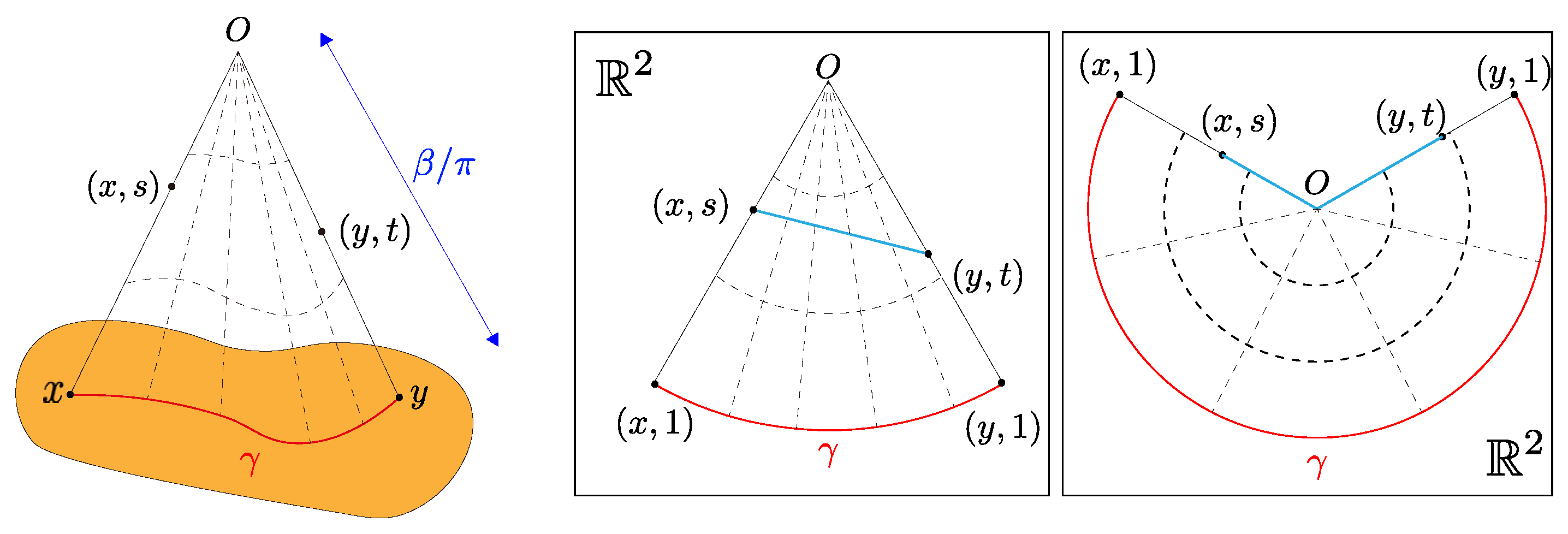
2.3. The Metric Cone

The metric cone is similar to ordinary cones (e.g., circle cones) in the sense that it is defined as a collection of line segments connecting an apex point to a given set. However, the metric cone has a notable property such that every point in the original set is embedded at an equal distance from the apex point and this is a desirable property for hierarchical structure extraction.

The metric cone has been studied as an analogy to the length metric spaces of the tangent cone for differential manifolds with singularities. Length metric space is a metric space where the distance between any two points is equal to the shortest curve length connecting them. Length metric space includes Euclidean spaces, normed vector spaces, manifolds (e.g., Poincaré ball; sphere), metric graphs, and many other metric spaces. Assume the original space Z is a length metric space, then the metric cone generated by Z is $X:=Z\times [0,1]/Z\times \left\{0\right\}$ with a distance function determined as follows:

$$\begin{array}{cc}\hfill {\tilde{d}}_{\beta }& \left(\right(x,s),(y,t\left)\right)\hfill \\ \hfill & =\beta \sqrt{t^2+s^2-2tscos\left(\pi min\left(d_Z(x,y)/\beta ,1\right)\right)}\hfill \end{array}$$

(5)

where $\beta >0$ is a hyperparameter corresponding to the length of the conical generatrix. Note that the metric cone itself also becomes a length metric space and it embeds the original space (i.e., the space is one dimension larger than the original space). The distance in the metric cone corresponds to the length of the shortest curve on the circle section (blue line segment(s) in the right two subfigures in Figure 1) whose bottom circumference is the distance of the original space Z and whose radius is $\beta$.

When the curvature is measured in the sense of CAT(k) property, a curvature measure for general length metric spaces, the curvature value k can be controlled by $\beta$. Other properties of the metric cone are examined in [27,28]. Because the metric cone can change the curvature of the space by changing parameter $\beta$, its usefulness has been reported in an analysis using the structure of the data space [24].

The metric $\tilde{g}$ of a metric cone is obtained by calculating the two-time derivative of the distance as follows (see Appendix A for more details):

$${\tilde{g}}_{(x,s)}=\left(\begin{array}{cc}{\pi }^2{s}^2{g}_x& 0\\ 0^{\top }& {\beta }^2\end{array}\right),$$

(6)

where $g_x$ represents the metric of Z at x. Combining this metric and the argument in Section 3.1, the algorithm of cone embedding can be described as Algorithm 1.

Algorithm 1 Learn the cone embedding {$(u,s)$}

Input:  graph $G=(V,E)$, cone’s hyperparameter $\beta$, learning rate $\eta$,     and the pre-trained embedding $\left\{x\right\}$ in original space Z Output:  the cone embedding {$(u,s)$}   1: calculate the distance matrix $D=\left(d_{ij}\right),d_{ij}=d_Z(x_i,x_j)$   2: minimize the softmax loss function:   (calculate efficiently by referencing the distance matrix D) $$\begin{array}{cc}\hfill L=& \sum _{\left(\right(u,s),(v,t\left)\right)\in E}log\frac{{exp}^{-{\tilde{d}}_{\beta }((u,s),(v,t))}}{\left({\sum }_{(v^{\prime },t^{\prime })\in N^c\left((u,s)\right)}exp\left(-{\tilde{d}}_{\beta }((u,s),(v^{\prime },t^{\prime }))\right)\right)}\hfill \end{array}$$ (7)   via Riemannian stochastic gradient descent: $$\begin{array}{c}\hfill (x,s)\leftarrow proj\left((x,s)-\eta {\tilde{g}}^{-1}\nabla L\right)\end{array}$$

The loss function (7) is defined to be smaller if the distance between nodes sharing an edge becomes smaller (by the numerator in the log) and the distance between nodes without an edge becomes larger (by the denominator in the log). Note that the distance for a metric cone is used here. Computation of the denominator can be reduced by random sampling of nodes for which no edges exist. Furthermore, the projection normalizes the embedding along the gradient so that it does not jump out of the metric cone when it is updated.

Instead of the exponential map of the metric cone, we use the first-order approximation using proj(x, s):

$$\begin{array}{c}\hfill proj(x,s)=\left\{\begin{array}{ccc}(x,s)& \mathrm{if}& ϵ<s<1-ϵ,\\ (x,1-ϵ)& \mathrm{if}& s\ge 1-ϵ,\\ (x,ϵ)& \mathrm{if}& s\le ϵ.\end{array}\right.\end{array}$$

(8)

2.4. Score Function of Hierarchy

The Poincaré embedding defines an index in [17], which is aimed to be an indicator of the hierarchical structure and depends on the distance from the origin:

$$\begin{array}{c}\hfill score(u,v)=-\alpha (\parallel v\parallel -\parallel u\parallel )d(u,v)\end{array}$$

(9)

This score function is penalized by the part after $\alpha$, so, if v is closer to the origin than u, then it is easier to obtain larger values. In other words, v is higher in the hierarchy than u (i.e., “u is a v” relationship holds). However, it is not appropriate to use this indicator for the Poincaré embedding. This model learns the embedding by maximizing (1), where

$$\begin{array}{c}\hfill d(x,y):=arcosh\left(1+\frac{{\parallel x-y\parallel }^2}{{(1-\parallel x\parallel }^2\left)\right(1-{\parallel y\parallel }^2)}\right).\end{array}$$

(10)

This loss function only depends on the distance between the two embeddings. However, an isometric transformation in the Poincaré ball exists, known as the Möbius transformation [29]. Möbius transformation is defined as a map $f:{\mathbb{B}}^n(\mathrm{open}\mathrm{unit}\mathrm{ball})\to {\mathbb{B}}^n$, which can be written as a product of the inversions of ${\overline{\mathbb{R}}}^n(:={\mathbb{R}}^n\cup \{\infty \})$ through a sphere S that preserves ${\mathbb{B}}^n$.

In contrast to the Poincaré ball, the isometric transformation on the metric cone does not exist when the coordinate in the original space is fixed (we prove this property in Appendix C). When we embed a graph into a metric cone, we define an indicator of the hierarchical structure by replacing the norm with a coordinate corresponding to the height of the cone (a one-dimensional parameter added to the original space):

$$\begin{array}{c}\hfill \mathrm{score}\left(\right(\mathbf{u},\mathrm{s}),(\mathbf{v},\mathrm{t}\left)\right)=-\alpha (s-t)d(\mathbf{u},\mathbf{v}).\end{array}$$

(11)

A point closer to the top of the cone is higher in the hierarchy, which is natural for representing hierarchical structure.

2.5. Using Pre-Trained Model for Computational Efficiency and Adaptivity for Adding Hierarchical Information

Consider a situation where we already have a trained graph embedding on a Euclidean space (e.g., LINE [14]) and we try to learn the embedding in a metric cone of Euclidean space to extract information about the hierarchical structure. In this case, we can reduce the computational cost by fixing the coordinates corresponding to the original Euclidean space and learn only the one-dimensional parameters corresponding to heights in a metric cone added to the original space because the metric cone is one dimension larger than the original space. The distance between each embedding in the original space is calculated beforehand, since no updates are made by learning except for the 1D parameter to be added. By referring to the pre-computed distances in the original space when calculating the distances between each embedding on the metric cone ($d_z(x,y)$ in Equation (5)) during training, we can reduce the amount of computation for the parts other than preprocessing, regardless of the dimension. In addition, because the embedding in the original Euclidean space is preserved, it can be used as an input to the neural network (when the task considers information about the hierarchy and the added one-dimensional parameters are also used as input) and can be easily applied to other tasks. However, other non-Euclidean embedding methods to extract hierarchical structures are not scalable because these methods cannot be applied directly to solve other tasks. For example, deep neural networks cannot use a non-Euclidean embedding as input because the sum of two vectors in the space and scalar product is not generally defined.

2.6. Comparison with Hierarchical Clustering

Although both cone embedding and hierarchical clustering aim to extract hierarchical structures, there is a clear difference between their problem settings. In hierarchical clustering, only leaves in a result tree (dendrogram) correspond to data points and other nodes correspond to created clusters. Thus, the problem setting differs significantly from cone embedding in which each node in a data graph corresponds to a pre-defined entity. As a result, hierarchical clustering cannot extract the hierarchy of nodes other than leaves while cone embedding can do. Moreover, the order of computational complexity is also different: hierarchical clustering requires $O\left(n^2\right)$, while cone embedding requires $O\left(\right|E\left|\right)$ ($\left|E\right|$: number of edges), making it suitable for extracting hierarchical structures in large graphs.

It has been also shown by [30] that the embedding of tree-structured (undirected) graph data can be done naturally in hyperbolic space, but graph data with hierarchical structure does not necessarily have a tree structure in general (e.g., there can be a cycle when a child node has two parents which have the same parent). Thus, the combination with hyperbolic embedding and hierarchical clustering may not be suitable in such cases. Cone embedding does not assume the tree structure and extracts the hierarchical structure by using the property that the closer to the origin O the shorter the distance between data points, so that embedding can be learned even in this situation.

3. Theory

In this section, we give theoretical proof as to why the spatial properties of the metric cone are suitable for extracting hierarchical structures.

3.1. Identifiability of the Heights in Cone Embedding

As mentioned above, for Poincaré embedding, there is an isometric transformation on the Poincaré ball and the heights of the learned hierarchy are not invariant to such transformation. Here, we show that such a phenomenon does not occur for the cone embedding, i.e., the heights of the hierarchy are (almost) uniquely determined from the distance between the embedded data points in a metric cone.

Let Z be an original embedding space (connected length metric space) and let X be a metric cone of Z with a parameter $\beta >0$. We assume that each data point $z_i\in Z(i=1,\dots ,n)$ has its specific “height” $t_i\in [0,1]$ in the metric cone X. Our proposed method embeds data points into a metric cone based on the estimated distances ${\tilde{d}}_{\beta }(x_i,x_j)(i,j=1,\dots ,n)$ and tries to compute the heights $t_1,\dots ,t_n$ as a measure of the hierarchy level. However, it is not evident whether these heights are identifiable only from the information of the original data points in Z and the distances ${\tilde{d}}_{\beta }(x_i,x_j)(i,j=1,\dots ,n)$ in the metric cone. The following theorem guarantees some identifiability. (A rigorous version of Theorem 1, including the precise meaning of “identifiable” in (a)–(c) and “general” in (b), is explained in Appendix C.)

Theorem 1.

(a) Let $n\ge 3$ and assume that $z_1,\dots ,z_n$ are not all aligned on a geodesic in Z. Then, the heights $t_1,\dots ,t_n$ are identifiable up to at most four candidates.

(b)

Let $n\ge 4$ and assume $z_1,\dots ,z_n$ and $t_1,\dots ,t_n$ take “general” positions and heights, respectively. Then, the heights $t_1,\dots ,t_n$ are identifiable uniquely.

(c)

If $d_Z(z_i,z_j)\ge \frac{\beta }{2}$ for all $i,j=1,\dots ,n,i\ne j$, then the heights $t_1,\dots ,t_n$ are identifiable uniquely.

Theorem 1(a) indicates that the candidates of heights are finite and we can expect the algorithm to converge to one of them, except for a very special data distribution in the original space Z. Moreover, by (b), even the uniqueness can be proved under very mild conditions. The statement in (c) implies that the uniqueness holds for arbitrary data distributions when we set $\beta$ sufficiently small.

Remark that the assumption of “general” positions in Theorem 1(b) is satisfied easily for most data distributions. For example, if both $z_1,\dots ,z_n\in {\mathbb{R}}^d$ and $t_1,\dots ,t_n\in [0,1]$ are i.i.d. from a probability distribution whose density function exists with respect to the Lebesgue measure, then it is easy to see the assumption holds almost surely and therefore the uniqueness of the solution is guaranteed. Note that, for $n=3$ under the same setting, there can be multiple solutions with a positive probability.

3.2. Variable Curvature

One of the essences of Poincaré embedding is that a negative curvature of the Poincaré sphere is suitable for embedding tree graphs. The curvature of a metric cone has a similar property, i.e., a metric cone has more negative curvature than the original space and, furthermore, the curvature can be controlled by hyperparameter $\beta$. We will verify these facts mathematically from two different aspects: (i) the scalar and the Ricci curvatures of a Riemannian manifold and (ii) the CAT(k) property of a length metric space.

First, assume the original space $\mathcal{M}$ is an n-dimensional Riemannian manifold with a metric g. Then the metric $\tilde{g}$ of the corresponding metric cone with $\beta$ can be defined except for the apex and it becomes as (6). Let $1,\dots ,n$ be coordinate indices corresponding to $x\in \mathcal{M}$ and 0 be the index corresponding to $s\in [0,1]$. The Ricci curvatures ${\tilde{R}}_{ij}$ and the scalar curvature $\tilde{R}$ at $(x,s)$ become

$$\begin{array}{cc}\hfill {\tilde{R}}_{\alpha \gamma }& =R_{\alpha \gamma }-{\pi }^2(n-1){\beta }^{-2}{\tilde{g}}_{\alpha \gamma },\hfill \end{array}$$

(12)

$$\begin{array}{cc}\hfill {\tilde{R}}_{\alpha 0}& ={\tilde{R}}_{0\alpha }={\tilde{R}}_{00}=0,\hfill \end{array}$$

(13)

$$\begin{array}{cc}\hfill \tilde{R}& =\{{\pi }^{-2}R-n(n-1){\beta }^{-2}\}{s}^{-2}\hfill \end{array}$$

(14)

where $\alpha ,\gamma$ are coordinate indices in $1,\dots ,n$ and $R_{ij}$ and R are the Ricci curvatures and the scalar curvature of $\mathcal{M}$, respectively. See Appendix B for the derivation of such curvatures. The scalar curvature and the Ricci curvatures ${\tilde{R}}_{\alpha \gamma }$ become more negative than (a constant times of) the original curvature for $\beta <\infty$ and $n\ge 2$. Moreover, the smaller value of $\beta$ makes the curvature more negative; thus, it becomes possible to control the curvature by tuning $\beta$. Note that, the closer to the apex, i.e., the smaller the value of s, the greater the change of the scalar curvature.

Second, assume the original space $\mathcal{M}$ is a length metric space. This does not require a differentiable structure and is more general than the Riemannian manifold. In this case, we cannot argue the curvatures using the Riemannian metric but the CAT(k) property can be used instead. In [24], they proved the curvature of the metric cone is more negative or equal to the curvature of the original space and it can be controlled by $\beta$ in the sense of the CAT(k) property.

4. Experiments

The claim in this paper is that “a hierarchical structure can be captured by adding a one-dimensional parameter and embedding it in a metric cone.” Therefore, we evaluate the proposed method in two experiments:

• Prediction of edge direction for artificially directed graphs;
• Estimation of the hierarchical score by humans for WordNet.

As a comparison, we compare the proposed method with two other methods: Poincaré embedding [17] and ordinary embedding in Euclidean space, which are known to capture the hierarchical structure of graphs. For Euclidean embedding, we use the distance from the mean of embedded data points as the hierarchical score in (8).

4.1. Prediction of Edge Direction for Directed Graphs

In this experiment, we estimate the orientation of directed edges for some simple graphs such that it is natural to think of the direction of the edges as representing the vertical relationship in the hierarchy.

4.1.1. Settings

We use the following three patterns of graphs with a naturally set hierarchical structure:

• Graphs generated by a growing random network model called the Barabási–Albert preferential attachment [31] with $m=2$, where m is the number of edges to attach from a new node to existing nodes;
• Complete k-ary tree;
• Concatenated tree of two complete k-ary sub-trees.

For the growing random network model, the hierarchy and the corresponding orientation is naturally defined by the order in which each node is attached. For each tree, node depth can be treated as its hierarchy. The concatenated tree is created by connecting the roots of two complete k-ary trees to a new node, which is then used as the new root. The concatenated tree is considered to study the effect of node degree on the cone embedding as will be explained below.

In this experiment, we learn the embedding of each directed graph. However, we use the information of directions only for evaluation and not for learning. For each directed edge of the learned graph, we estimate the direction by the computed hierarchical scores $score(u,v)$:

$$\mathrm{total\_score}=\sum _{(u,v)\in E}sc\tilde{o}re(u,v)/\left|E\right|$$

(15)

$$\begin{array}{cc}\hfill sc\tilde{o}re(hypo,hype)& =\left\{\begin{array}{cc}1& score(hypo,hype)>0\\ 0& \mathrm{otherwise}\end{array}\right.\hfill \\ \hfill \mathrm{where}hype:& \mathrm{higher}\mathrm{hierarchy}\mathrm{node}\hfill \\ \hfill hypo:& \mathrm{lower}\mathrm{hierarchy}\mathrm{node}\hfill \end{array}$$

(16)

Hyperparameters were set as follows. First, the number of negative samplings was set to 5; while increasing the number of negative samplings increases the amount of computation, the effect on accuracy was not significant, so it was set small. Learning was performed for values of $\beta$ at 0.1, 0.5, 1, and 5, and the best results are described in

Table 1. Result for prediction of edge direction for directed graphs. (We list accuracy and standard deviation. Compared to other methods, cone embedding tends to extract the hierarchical structure correctly even when the number of nodes increases).

Model	Barabási–Albert	Complete k-Ary-Tree		Concatenated k-Ary Trees
	(Nodes: 100)	k = 3 (121)	k = 5 (781)	k = 3 (81)	k = 5 (313)
Cone	0.936 (sd: 0.005)	0.787 (0.049)	0.799 (0.037)	0.783 (0.045)	0.744 (0.056)
Euclidean	0.181 (0.004)	0.074 (0.088)	0.127 (0.020)	0.190 (0.136)	0.155 (0.031)
Poincaré	0.957 (0.012)	0.935 (0.015)	0.351 (0.022)	0.880 (0.060)	0.606 (0.043)

. Here all nodes and edges of the graph are used for both training and evaluation.

4.1.2. Results

The experimental results are shown in Table 1 and the cone embedding shows overall good and stable estimation accuracy for hierarchies. Examples in Figure 2 depict how each graph is embedded in a metric cone. Other existing methods may outperform for sparse trees (small degree of each node) but this method has an advantage for dense trees. The reason for the instability in the accuracy of Poincaré embedding may be the lack of invariance with respect to the equidistance transformation, as we have explained. The main reason for the poor hierarchical estimation accuracy of Euclidean embedding is that the root or higher hierarchical nodes are embedded apart from the cluster of other nodes as in Figure 3. As a result, the root node becomes far from the origin of the embedded space.

For the Barabási–Albert model, the relationship between the (added 1D) coordinates of the cone hierarchy and the order is shown in Figure 4. We can see that there is a strong relationship between the degree and the hierarchy. This raises the suspicion that the degree of the node alone determines the hierarchy of the embedding. However, the fact that the cone embedding provides high estimation accuracy even for the concatenated trees with low root degree indicates that this is not true.

4.2. Embedding Taxonomies

Following an experiment in [17] for the Poincaré embedding, we evaluate the embedding accuracy of the hierarchical structure using WordNet. To verify this, we embed the nouns in WordNet into a metric cone and use the score function (“total_score” described in Section 4.1). Note that hyperparameter $\alpha$ was set to ${10}^3$. The output of this score function and the correlation coefficient of the HyperLex dataset’s score (evaluated manually whether a word is a hyponym of another word) are used to evaluate the ability to represent the hierarchical structure of the model.

In addition to hierarchical scores, we also evaluate the accuracy of graph embedding. We use mean rank and mean average precision, which are commonly used in existing graph embedding accuracy, as evaluation metrics. The mean rank is calculated for each node as the rank of its neighbors when sorted in order of distance. The mean average precision is calculated as follows:

• Fix one node and calculate the distance to all other nodes.
• Consider the node adjacent to the fixed node as the correct data, and calculate the average precision for this correct data using the distance as the confidence score.
• Perform the above two operations on all the nodes and take the average.

The embedding accuracy (mean rank (MR) and mean average precision (MAP)) and correlation coefficients are also shown in

Table 2. MAP, mean rank (MR), Hyperlex score (correlation efficient) and computation time for WordNet. Cone embedding is trained from Euclidean embedding, e.g., in 10-dims cone embeddings, we trained additional 1-dim parameters from 10 dims Euclidean embeddings. For MR and comp. time lower is better, and for MAP and corr. higher is better.

Model	Evaluation Metric	Dimensions
		10	20	50	100
Euclidean	MR	1681.18	583.75	233.7	162.43
	MAP	0.07	0.12	0.25	0.37
	corr	0.25	0.34	0.38	0.39
	comp. time	976.48	984.72	2169.1	2095.7
Poincaré	MR	1306.22	1183.29	1112.42	1096.08
	MAP	0.09	0.13	0.14	0.16
	corr	0.07	0.08	0.09	0.09
	comp. time	2822.99	1807.73	3954	2241.7
Cone	MR	426.75	675.09	777.3	910.51
($\beta =1.0$)	MAP	0.10	0.08	0.07	0.06
	corr	0.39	0.40	0.40	0.40
	comp. time	177.94	174.67	168.33	187.83
Cone	MR	688.85	143.23	74.39	51.32
($\beta =5.0$)	MAP	0.07	0.23	0.50	0.57
	corr	0.35	0.35	0.37	0.38
	comp. time	176.04	171.21	168.7	189.89

. Note that all of the graph data are used for training and the results are evaluated according to the accuracy with which the graph is reconstructed from the learned embedding. Because the same data are used for training and evaluation, we evaluate the fittingness of the embedding method to the data.

The table shows that our proposed model improves the score and captures the hierarchical structure better than other embedding methods. Furthermore, “comp. time” represents the time taken to train the embedding (1000 epochs); for cone embedding, it represents the time taken to train in one additional dimension (100 epochs). From the table, we can see that our method is efficient in learning and does not vary with the dimension of the embedding. The result also shows that the optimal $\beta$ value can depend on the dimension. Because larger $\beta$ corresponds to smaller curvature, the proposed method seems to perform better when embedding in a smaller curvature space if the dimension becomes higher. For the same reason, Euclidean embedding is considered to perform better than Poincare embedding in high dimensions due to their zero curvature. Tuning of $\beta$ is necessary because the optimal value also varies depending on the training data. In this case, the search was done in $\beta =0.1,0.5,1.0,5.0$ but a finer search may improve the accuracy.

Furthermore, an example visualization of the hierarchical structure of the embedding vectors obtained by the training is shown in Figure 5. As the figure illustrates, the closer the coordinate corresponding to the height in the cone is to zero (closer to the top of the cone), the higher the noun in the hierarchy is located in the embedded representation. For visualization, the embedding vectors in Euclidean space were reduced to two dimensions by principal component analysis.

5. Discussion and Future Works

In this study, we have demonstrated that a graph embedding in a metric cone that is a dimension larger than the existing embedding methods has the following advantages: (1) we naturally define an index (score function) as an indicator of hierarchy, (2) the proposed method has some adaptivity since it can introduce the hierarchy into various pre-trained models by learning only newly added 1D parameters, and (3) thus, the optimization is computationally inexpensive and stable. By optimizing the 1D parameters, we have shown that the proposed method also has the flexibility to optimize the curvature to enhance the accuracy as well as other methods. Since the metric cone is defined as a space with +1 dimension with respect to the original metric space, it is also possible to learn cone embedding in the same way even when the original space is Poincaré. We demonstrated the feasibility of extracting the hierarchical structure using solely the additional space by fixing the original space and learning its embedding.

It is worth noting that an alternative approach involves directly embedding the graph into the metric cone by learning an embedding that includes the source space. However, the constraint of learning in one dimension offers some advantages. For instance, the metric cone is defined as a space with +1 dimension with respect to the original metric space, which allows for the learning of cone embedding in the same way for any general original spaces, including the Poincaré space. The independence of the optimization algorithm from the original embedding space results in a more stable computation. For example, the cone embedding performed best or fairly for overall settings while the Poincaré embedding performed very poorly in some experimental settings. Moreover, the tuning of hyperparameters such as $\beta$ for embedding can be performed independently from the original embedding.

Future research topics include (1) efficient optimization of curvature, (2) development of an embedding method to update existing embeddings in learning, and (3) discovery of applications to other tasks. In this study, we measured the improvement of the accuracy of curvature optimization by the grid search. However, more efficient methods, such as gradient-based methods, can be used to optimize the embedding space. We also learned embedding in a metric cone under the constraint of not updating existing embeddings. This constraint can cause the optimization to fall into a local solution. Therefore, to optimize the entire embedding, an efficient method of optimizing functions on a metric cone (or Riemannian manifold) should be developed in future work.

References

1. Zhang, J.; Ackerman, M.S.; Adamic, L. Expertise networks in online communities: Structure and algorithms. In Proceedings of the 16th international Conference on World Wide Web, Banff, AB, Canada, 8–12 May 2007; pp. 221–230. [Google Scholar]
2. De Choudhury, M.; Counts, S.; Horvitz, E. Social media as a measurement tool of depression in populations. In Proceedings of the 5th Annual ACM Web Science Conference, Paris, France, 2–4 May 2013; pp. 47–56. [Google Scholar]
3. Page, L.; Brin, S.; Motwani, R.; Winograd, T. The PageRank Citation Ranking: Bringing Order to the Web; Technical Report; Stanford InfoLab, Stanford University: Stanford, CA, USA, 1999. [Google Scholar]
4. Barabasi, A.L.; Oltvai, Z.N. Network biology: Understanding the cell’s functional organization. Nat. Rev. Genet. 2004, 5, 101–113. [Google Scholar] [CrossRef] [PubMed]
5. Yahya, M.; Berberich, K.; Elbassuoni, S.; Weikum, G. Robust question answering over the web of linked data. In Proceedings of the 22nd ACM International Conference on Information & Knowledge Management, San Francisco, CA, USA, 27 October–1 November 2013; pp. 1107–1116. [Google Scholar]
6. Hoffart, J.; Milchevski, D.; Weikum, G. STICS: Searching with strings, things, and cats. In Proceedings of the 37th International ACM SIGIR Conference on Research & Development in Information Retrieval, Gold Coast, Queensland, Australia, 6–11 July 2014; pp. 1247–1248. [Google Scholar]
7. Klimovskaia, A.; Lopez-Paz, D.; Bottou, L.; Nickel, M. Poincaré maps for analyzing complex hierarchies in single-cell data. Nat. Commun. 2020, 11, 2966. [Google Scholar] [CrossRef] [PubMed]
8. Kipf, T.N.; Welling, M. Semi-supervised classification with graph convolutional networks. arXiv 2016, arXiv:1609.02907. [Google Scholar]
9. Ribeiro, L.F.; Saverese, P.H.; Figueiredo, D.R. struc2vec: Learning node representations from structural identity. In Proceedings of the 23rd ACM SIGKDD International Conference on Knowledge Discovery and Data Mining, Halifax, NS, Canada, 13–17 August 2017; pp. 385–394. [Google Scholar]
10. Hamilton, W.; Ying, Z.; Leskovec, J. Inductive representation learning on large graphs. Adv. Neural Inf. Process. Syst. 2017, 30, 1025–1035. [Google Scholar]
11. Goyal, P.; Ferrara, E. Graph embedding techniques, applications, and performance: A survey. Knowl. Based Syst. 2018, 151, 78–94. [Google Scholar] [CrossRef]
12. Grover, A.; Leskovec, J. node2vec: Scalable feature learning for networks. In Proceedings of the 22nd ACM SIGKDD International Conference on Knowledge Discovery and Data Mining, San Francisco, CA, USA, 13–17 August 2016; pp. 855–864. [Google Scholar]
13. Cao, S.; Lu, W.; Xu, Q. Grarep: Learning graph representations with global structural information. In Proceedings of the 24th ACM International on Conference on Information and Knowledge Management, Melbourne, VIC, Australia, 19–23 October 2015; pp. 891–900. [Google Scholar]
14. Tang, J.; Qu, M.; Wang, M.; Zhang, M.; Yan, J.; Mei, Q. Line: Large-scale information network embedding. In Proceedings of the 24th International Conference on World Wide Web, Florence, Italy, 18–22 May 2015; pp. 1067–1077. [Google Scholar]
15. Sun, Z.; Chen, M.; Hu, W.; Wang, C.; Dai, J.; Zhang, W. Knowledge Association with Hyperbolic Knowledge Graph Embeddings. In Proceedings of the 2020 Conference on Empirical Methods in Natural Language Processing (EMNLP), Association for Computational Linguistics, Online, 16–20 November 2020; pp. 5704–5716. [Google Scholar] [CrossRef]
16. Rezaabad, A.L.; Kalantari, R.; Vishwanath, S.; Zhou, M.; Tamir, J. Hyperbolic graph embedding with enhanced semi-implicit variational inference. In Proceedings of the International Conference on Artificial Intelligence and Statistics, PMLR, Virtual, 13–15 April 2021; pp. 3439–3447. [Google Scholar]
17. Nickel, M.; Kiela, D. Poincaré embeddings for learning hierarchical representations. In Proceedings of the Advances in Neural Information Processing Systems, Long Beach, CA, USA, 4–9 December 2017; pp. 6338–6347. [Google Scholar]
18. Zhang, Z.; Cai, J.; Zhang, Y.; Wang, J. Learning hierarchy-aware knowledge graph embeddings for link prediction. In Proceedings of the AAAI Conference on Artificial Intelligence, New York, NY, USA, 7–12 February 2020; Volume 34, pp. 3065–3072. [Google Scholar]
19. Chami, I.; Wolf, A.; Juan, D.C.; Sala, F.; Ravi, S.; Ré, C. Low-Dimensional Hyperbolic Knowledge Graph Embeddings. In Proceedings of the 58th Annual Meeting of the Association for Computational Linguistics, Association for Computational Linguistics, Online, 5–10 July 2020; pp. 6901–6914. [Google Scholar] [CrossRef]
20. Dhingra, B.; Shallue, C.; Norouzi, M.; Dai, A.; Dahl, G. Embedding Text in Hyperbolic Spaces. In Proceedings of the Twelfth Workshop on Graph-Based Methods for Natural Language Processing (TextGraphs-12), Association for Computational Linguistics, New Orleans, LA, USA, 6 June 2018; pp. 59–69. [Google Scholar] [CrossRef]
21. Nickel, M.; Kiela, D. Learning Continuous Hierarchies in the Lorentz Model of Hyperbolic Geometry. In Proceedings of the Machine Learning Research, PMLR, Stockholmsmässan, Stockholm, Sweden, 10–15 July 2018; Volume 80, pp. 3779–3788. [Google Scholar]
22. Ganea, O.; Becigneul, G.; Hofmann, T. Hyperbolic Entailment Cones for Learning Hierarchical Embeddings. In Proceedings of the Machine Learning Research, PMLR, Stockholmsmässan, Stockholm, Sweden, 10–15 July 2018; Volume 80, pp. 1646–1655. [Google Scholar]
23. Sala, F.; De Sa, C.; Gu, A.; Ré, C. Representation tradeoffs for hyperbolic embeddings. In Proceedings of the International Conference on Machine Learning, PMLR, Stockholm, Sweden, 10–15 July 2018; pp. 4460–4469. [Google Scholar]
24. Kobayashi, K.; Wynn, H.P. Empirical geodesic graphs and CAT (k) metrics for data analysis. Stat. Comput. 2020, 30, 1–18. [Google Scholar] [CrossRef]
25. Wilson, R.C.; Hancock, E.R.; Pekalska, E.; Duin, R.P. Spherical and Hyperbolic Embeddings of Data. IEEE Trans. Pattern Anal. Mach. Intell. 2014, 36, 2255–2269. [Google Scholar] [CrossRef] [PubMed]
26. Chami, I.; Ying, Z.; Ré, C.; Leskovec, J. Hyperbolic Graph Convolutional Neural Networks. In Proceedings of the Advances in Neural Information Processing Systems; Wallach, H., Larochelle, H., Beygelzimer, A., d’Alché-Buc, F., Fox, E., Garnett, R., Eds.; Curran Associates, Inc.: Red Hook, NY, USA, 2019; Volume 32. [Google Scholar]
27. Sturm, K.T. Probability measures on metric spaces of nonpositive curvature. In Proceedings of the Heat Kernels and Analysis on Manifolds, Graphs, and Metric Spaces: Lecture Notes A Quart, Program Heat Kernels, Random Walks, Analysis Manifolds Graphs, Emile Borel Cent, Henri Poincaré Institute, Paris, France, 16 April–13 July 2002; Volume 338, p. 357. Available online: https://bookstore.ams.org/conm-338 (accessed on 24 February 2023).
28. Deza, M.M.; Deza, E. Encyclopedia of Distances; Springer: Berlin/Heidelberg, Germany, 2009; pp. 1–583. [Google Scholar]
29. Loustau, B. Hyperbolic geometry. arXiv 2020, arXiv:2003.11180. [Google Scholar]
30. Sarkar, R. Low distortion delaunay embedding of trees in hyperbolic plane. In Proceedings of the International Symposium on Graph Drawing, Eindhoven, The Netherlands, 21–23 September 2011; pp. 355–366. [Google Scholar]
31. Barabasi, A.L.; Albert, R. Emergence of Scaling in Random Networks. Science 1999, 286, 509–512. [Google Scholar] [CrossRef] [PubMed]
32. Janson, S. Riemannian geometry: Some examples, including map projections. Notes. 2015. Available online: http://www2.math.uu.se/~svante/papers/sjN15.pdf (accessed on 24 February 2023).
33. Cox, D.; Little, J.; OShea, D. Ideals, Varieties, and Algorithms: An Introduction to Computational Algebraic Geometry and Commutative Algebra; Springer Science & Business Media: Berlin/Heidelberg, Germany, 2013. [Google Scholar]
Figure 1. The left figure depicts a conceptual image of an original space and its metric cone. A circle section to compute the distance in the metric cone is depicted in the middle figure (when the apex angle < π ) and the right figure (when the apex angle π ).
Mathematics 11 02294 g001
Figure 2. Graphs used for training: (left) model trained by Barabási–Albert model, (middle) complete k-ary tree, (right) concatenated tree of two complete k-ary trees. The x- and y-axes represent embedding in Euclidean space, which is dimensionally reduced to two dimensions by principal component analysis, and the z-axis represents the height in the metric cone (coordinates representing the hierarchy).
Mathematics 11 02294 g002
Figure 3. An embedding of the complete k-ary tree ( k = 3 ). Each point is plotted by the 3D Euclidean embedding and the color represents length of shortest path from root node (the bluer the color, the higher the hierarchy).
Mathematics 11 02294 g003
Figure 4. Plot of the hierarchy value of each node in a cone embedding (a newly added one-dimensional parameter) against their node degree.
Mathematics 11 02294 g004
Figure 5. Visualization of wordnet hypernym and hyponym relations by cone embedding (beta: 1.0) learned from 10 to dimensional Euclidean embedding. The right figure is for the car and the left figure is for sport, describing the relationship with one higher or lower word. (In the visualization, all nodes are visualized, but only some of the word names corresponding to each node are shown. The original embedding vector (Euclidean in this case) is also made two-dimensional by PCA.)
Mathematics 11 02294 g005