Novel Graph Neighborhoods Emerging from Ideals

Abstract

Rough set theory is a mathematical approach that deals with the problems of uncertainty and ambiguity in knowledge. Neighborhood systems are the most effective instruments for researching rough set theory in general. Investigations on boundary regions and accuracy measures primarily rely on two approximations, namely lower and upper approximations, by using these systems. The concept of the ideal, which is one of the most successful and effective mathematical tools, is used to obtain a better accuracy measure and to decrease the boundary region. Recently, a generalization of Pawlak’s rough set concept has been represented by neighborhood systems of graphs based on rough sets. In this research article, we propose a new method by using the concepts of the ideal and different neighborhoods from graph vertices. We examine important aspects of these techniques and produce accuracy measures that exceed those previously = reported in the literature. Finally, we show that our method yields better results than previous techniques utilized in chemistry.

1. Introduction

Mathematicians come up with brand new hypotheses on a daily basis because of the significance of mathematically expressing ambiguous ideas that cannot be defined by traditional reasoning. Probability and statistics are the subjects of some of the most influential and well-known theories.

Economics, healthcare, engineering, business and other research fields face the same challenge: how to model uncertainty in scientific data. The uncertainties that appear in these fields can take a wide variety of shapes, making it difficult for traditional approaches to yield positive results. It is commonly known that rough set theory provides ways that can be helpful in identifying sources of uncertainty. Pawlak [1,2] presented uncertainty as a mathematical perspective that is concerned with the vagueness and fuzziness of approximate information. The theory’s basic concept is approximation operators, which are named in terms of equivalence classes. However, there are modern-day uses where such an equivalence relation falls short. As a result, various generalizations of equivalence relations have been proposed [3,4,5], including tolerance relations, preorder relations and arbitrary binary relations. Data analysis in biology, chemistry and engineering, etc. are only a few of the many domains that can benefit from it [6,7,8,9].

Lin and Yao [10,11] used neighborhood methods to evaluate granules as they studied rough sets. Allam et al. and Abd El-Monsef et al. [12,13] introduced the j-neighborhood space, which represents a generalized type of neighborhood spaces, and proposed mixed neighborhood systems to approximate rough sets. Amer et al. [7] modified and generalized the j-approximations in the j-neighborhood space to produce new j-nearly approximations as mathematical tools. Several rough set models based on the j-neighborhood space and other rough set models based on the j-adhesion neighborhood space were generalized by Atef et al. [14]. $C_j$-neighborhoods, which are dependent on the inclusion relations between j-neighborhoods, were defined and studied by Al-Shami [6]. Using the j-neighborhoods, Al-Shami and Ciucci [15] investigated the ideas of $S_j$-neighborhoods and their characteristics, where $j\in \left\{r,l,〈r〉,〈l〉,u,i,〈u〉,〈i〉\right\}$.

One of the key research topics in the subject of mathematics is the ideal, which Kuratowski [16] initially defined. An ideal is a non-empty collection of sets that is closed by the finite additivity and the hereditary condition. Recently, there has been a sharp increase in interest in various idealized versions of rough sets models. The advantage of including the concept of the ideal in this theory is that it increases lower approximations and decreases upper approximations, which reduces the vagueness (uncertainty) of a notion to uncertainty areas at their borders. As a result, the boundary region is reduced, and the accuracy measure is enhanced. Additionally, the ideal can be considered as a class of objects in the information system that has certain conditions and can be studied to arrive at new granulations on data collected from real-life problems.

Authors have also produced non-granular rough approximations over general approximations by using ideals. These relations based on rough sets aim to yield fine properties analogous to those of classical rough approximations. Firstly, the concept of ideals with right neighborhoods was used by Kandil et al. [17] to expand Pawlak’s approximations. Mathematicians demonstrated that, in comparison with Pawlak’s approach [2] and Yao’s method [11], their results minimize the boundary region. Then, Hosny [18] generated different topologies using the concept of the ideal. The author constructed new j-approximations using these topologies and demonstrated that the nomenclature of j-approximations extends to the approximations where $j\in \left\{r,l,〈r〉,〈l〉,u,i,〈u〉,〈i〉\right\}$. Then, based on the concept of the ideal and different neighborhoods, Hosny et al. [19] investigated a type of approximation and compared it with previous ones.

Graph theory [20,21] is an extremely well-known area that has many applications in various fields, including, but not limited to, advertising, management, commerce, information transfer, biology and physics. The theory makes it possible to break down the problem into manageable pieces and tackle them in a methodical, orderly fashion. A graph is a collection of points called vertices and connections called edges that link the points or merely the vertices. A graph is simple if it has no loop (i.e., a loop is an edge that connects a vertex to itself) and no pair of its links joins the same pair of vertices. Graphs can be defined mathematically as a tuple $G=\left(V,E\right)$, where $V$ and $E$ are sets of vertices and edges, respectively. Mathematicians have carried out extensive work studying graph theory and its many applications. Two studies that use graph theory to depict binary relations are those by Jarvinen [22] and Chen and Li [23]. In both cases, the mathematicians used a directed, basic graph to represent relationships. Starting from their studies, inquiries into the connections between several crude set theoretic notions and those of graph theory have emerged.

In 2018, Nada et al. [24] began studying the neighborhood system on rough sets, which led them to focus on the topological structure of graphs that correctly describe neighborhoods. Structures such as the human heart and self-similar fractals were then represented using the rough sets on graphs and the neighborhood systems on distinct fields, both of which are employed in medicine and physics. El-Atik et al. [25,26,27] defined the neighborhood system including a vertex of a graph and investigated its properties. Finally, utilizing the ideal and the j-neighborhoods for any subgraph of a given graph, Güler [28] constructed and explored a novel class of approximations, where $j\in \left\{r,l,〈r〉,〈l〉,u,i,〈u〉,〈i〉\right\}$.

The main motivation of our study is to investigate the relations between rough sets and graphs. In addition, we aim to obtain a better accuracy measure based on the concept of the ideal by using new lower and upper approximations on graphs. Hence, we minimized the boundary region by decreasing the upper approximations and increasing the lower approximations. Moreover, we examined a real-life problem to show that our approach yielded a better accuracy measure than the measures previously reported in the literature.

The present study is grounded in the concepts of rough sets, ideals and neighborhood systems. This study consists of four sections. Section 1 comprises the introduction. In Section 2, we present the definitions and theorems that are used throughout the article. In Section 3, we define a new class of approximations called $I$-$S$-$j$-approximations, where $j\in \left\{r,l,〈r〉,〈l〉,u,i,〈u〉,〈i〉\right\}$, by using the concept of the ideal and the j-neighborhoods for any subgraph of a given graph. Then, we study the relationships between them. In addition, we formulate the concepts of the $I$-$S$-$j$-boundary region and the $I$-$S$-$j$-accuracy of approximations of a subgraph. In Section 4, we define the $I$-$C$-$j$-lower and upper approximations, the $I$-$C$-$j$-boundary region and the $I$-$C$-$j$-accuracy measure of a subgraph $H$ of $G$ by using ideals and $C_j$-neighborhoods. Moreover, we tackle the relationship between these notions through examples and a taxonomy of their properties, and we also compare approximations. In the end, we summarize all comparisons and present examples to support our approach.

2. Preliminaries

In this section, we present the concepts of rough sets, graph theory and neighborhood.

Definition 1.

Let $X$ be a non-empty set. Then, a family of sets $I\subseteq P\left(X\right)$ is said to be an ideal in $X$ if [16]:

(a) 

$A,B\in I$ imply $A\cup B\in I$,

(b) 

$A\in I$ and $B\subset A$ imply $B\in I$.

Definition 2.

A relation $R$ from a set $U$ to itself is a subset of $U\times U$ and is a binary operation on $U.$ In this context, $\left(x,y\right)\in R$ is written as $xRy$ to express that $x$ is $R$-related on $y.$ Moreover, an after set (resp. fore set) of an element $x\in U$ is the class $xR=\left\{y\in U:xRy\right\}$. (resp. $Rx=\left\{y\in U:yRx\right\}$). $xR$ (resp. $Rx)$ can also be interpreted as the right neighborhood (resp. right neighborhood) of $x$ [29].

Definition 3.

The binary relation $R$ on a set $U$ is called [29]:

(a) 

Serial, if for every $x\in U,$ $\exists y\in U$ such that $xRy,$ i.e., $xR\ne \varnothing ;$

(b) 

Inverse serial, if for every $x\in U,$ $\exists y\in U$ such that $yRx,$ i.e., $x\in yR;$

(c) 

Reflexive, if for every $x\in U,$ $xRx;$

(d) 

Symmetric, if for every $x,y\in U$ and $xRy,$ then $yRx;$

(e) 

Transitive, if for every $x,y,z\in U$, $xRy$ and y$Rz,$ then $xRz;$

(f) 

Pre-order, if it is a reflexive and transitive relation;

(g) 

Equivalence, if it is a reflexive, symmetric and transitive relation.

Definition 4.

Let $U$ be a finite non-empty set, consider $R$ to be an equivalence relation on $U$ and let $U/R$ be the family of all equivalence classes of $R$ such that ${\left[x\right]}_R$ denotes an equivalence class in $R$ that contains an element $x\in U.$ The pair $P=\left(U,R\right)$ is called the Pawlak approximation space. Moreover, for any $X\subseteq U$, the Pawlak-lower approximations and Pawlak-upper approximations of $X$ are defined by [1]:

(a) 

$\underset{¯}{Apr}\left(X\right)=\left\{x\in U:{\left[x\right]}_R\subseteq X\right\}$;

(b) 

$\overline{Apr}\left(X\right)=\left\{x\in U:{\left[x\right]}_R\cap X\ne \varnothing \right\}$.

Later, Yao [11] generalized lower and upper approximations using binary relations with after sets, as showed in the following definitions:

Definition 5.

Let R be a binary relation on a finite non-empty set U and $X\subseteq U$. The lower approximations and upper approximations of $X$ are defined by [11]:

(a) 

$\underset{\_}{R}\left(X\right)=\left\{x\in U:xR\subseteq X\right\}$;

(b) 

$\overline{R}\left(X\right)=\left\{x\in U:xR\cap X\ne \varnothing \right\}$.

Definition 6.

Consider that R represents any binary relation on a finite non-empty set U and $X\subseteq U$. The boundary region and accuracy of approximation of X are defined by [11]:

(a) 

$BD{N}_R\left(X\right)=\overline{R}\left(X\right)-\underset{\_}{R}\left(X\right)$;

(b) 

${\sigma }_R=\frac{\left|\underset{\_}{R}\left(X\right)\right|}{\left|\overline{R}\left(X\right)\right|}$. where $\overline{R}\left(X\right)\ne \varnothing .$

Proposition 1.

Let $R$ be an equivalence relation on a non-empty set $U$ and $X,Y\subseteq U$. Then, the following properties apply [1,2]:

(L1) $\underset{\_}{R}\left(X\right)={\left(\overline{R}\left(X^c\right)\right)}^c;$

(L2) $\underset{\_}{R}\left(U\right)=U;$

(L3) $\underset{\_}{R}\left(X\right)\cup \underset{\_}{R}\left(Y\right)\subseteq \underset{\_}{R}\left(X\cup Y\right)$;

(L4) $\underset{\_}{R}\left(X\cap Y\right)=\underset{\_}{R}\left(X\right)\cap \underset{\_}{R}\left(Y\right)$;

(L5) If $X\subseteq Y$, then $\underset{\_}{R}\left(X\right)\subseteq \underset{\_}{R}\left(Y\right)$;

(L6) $\underset{\_}{R}\left(\varnothing \right)=\varnothing$;

(L7) $\underset{\_}{R}\left(X\right)\subseteq X$;

(L8) $\underset{\_}{R}\left(\underset{\_}{R}\left(X\right)\right)$ = $\underset{\_}{R}\left(X\right)$;

(L9) $\underset{\_}{R}$($\overline{R}\left(X\right))=\underset{\_}{R}\left(X\right)$;

(U1) $\overline{R}\left(X\right)={\left(\underset{\_}{R}\left(X^c\right)\right)}^c;$

(U2)$\overline{R}$(∅) = ∅;

(U3) $\overline{R}\left(X\right)\cup \overline{R}\left(Y\right)=\overline{R}\left(X\cup Y\right)$;

(U4) $\overline{R}\left(X\cap Y\right)\subseteq \overline{R}\left(X\right)\cap \overline{R}\left(Y\right)$;

(U5) If $X\subseteq Y$, then $\overline{R}\left(X\right)\subseteq \overline{R}\left(Y\right)$;

(U6) $\overline{R}\left(U\right)=U$;

(U7) $X\subseteq \overline{R}\left(X\right)$;

(U8) $\overline{R}\left(\overline{R}\left(X\right)\right)=\overline{R}\left(X\right)$;

(U9) $\underset{\_}{R}\left(\overline{R}\left(X\right)\right)=\overline{R}\left(X\right)$.

If $R$ is a binary relation according to Proposition 1, only the properties $L1$–$5$ and $U1$–$5$ are satisfied.

Definition 7.

Let $G=\left(V,E\right)$ be a graph. The $N_j$-neighborhood of $v\in V$ (briefly $N_j\left(v\right)$) is defined under the binary relation $R$ on $V$, where $j\in J=\left\{r,l,〈r〉,〈l〉,u,i,〈u〉,〈i〉\right\}$, as follows [12,13]:

(a) 

$N_r\left(v\right)=\left\{w\in V:vRw\right\}$;

(b) 

$N_l\left(v\right)=\left\{w\in V:wRv\right\}$;

(c) 

;

(d) 

(v) = $\left\{\begin{array}{cc}{{\displaystyle \cap }}_{v\in N_l\left(w\right)}{N}_l\left(w\right)& \exists N_l\left(w\right)containingv\\ \varnothing & otherwise\end{array}\right.$;

(e) 

$N_u\left(v\right)=N_r\left(v\right)\cup N_l\left(v\right)$;

(f) 

$N_i\left(v\right)=N_r\left(v\right)\cap N_l\left(v\right)$;

(g) 

;

(h) 

.

In the following definition, the $N_j$-neighborhood for $j\in J$ and the ideal are used to define the concept of $I_{N_j}$-lower approximations and $I_{N_j}$-upper approximations.

Definition 8.

Let $G=\left(V,E\right)$ be a graph and $H=\left(V\left(H\right),E\left(H\right)\right)$ be a subgraph of $G$ and $I$ be an ideal on $G$. For $j\in J,$ the $I_{N_j}$-lower approximations and $I_{N_j}$-upper approximations are defined as [28]:

(a) 

${\underset{\_}{N}}_j^I\left(V\left(H\right)\right)=\left\{v\in V:N_j\left(v\right)\cap V{\left(H\right)}^{ı}\in I\right\}$;

(b) 

${\overline{N}}_j^I\left(V\left(H\right)\right)=V\left(H\right)\cup \left\{v\in V:N_j\left(v\right)\cap V\left(H\right)\notin I\right\}$.

Definition 9.

Let $G=\left(V,E\right)$ be a graph and $H=\left(V\left(H\right),E\left(H\right)\right)$ be a subgraph of $G$ and $I$ be an ideal on $G$. Then for $j\in J$, the $I_{N_j^{*}}$-lower approximations and $I_{N_j^{*}}$-upper approximations are defined respectively by [28]:

(a) 

${\underset{\_}{N}}_j^{*I}\left(V\left(H\right)\right)=V\left(H\right)\cap {\underset{\_}{N}}_j^I\left(V\left(H\right)\right)$;

(b) 

${\overline{N}}_j^{*I}\left(V\left(H\right)\right)=V\left(H\right)\cup {\overline{N}}_j^I\left(V\left(H\right)\right)$.

In the following definition, the concept of the ideal and Definition 9 are used to present the concept of $I_{N_j^{*}}$-boundary regions and $I_{N_j^{*}}$-accuracy measures.

Definition 10.

Let $G=\left(V,E\right)$ be a graph and $H=\left(V\left(H\right),E\left(H\right)\right)$ be a subgraph of $G$ and $I$ be an ideal on $G$. Then for $j\in J$, the $I_{N_j{}^{*}}$-boundary regions and $I_{N_j{}^{*}}$-accuracy of approximations of $V\left(H\right)$ are defined by [28]:

(a) 

$B_{N_j^{*}}^I\left(V\left(H\right)\right)={\overline{N}}_j^{*I}\left(V\left(H\right)\right)-{\underset{\_}{N}}_j^{*I}\left(V\left(H\right)\right)$;

(b) 

${\sigma }_{N_j^{*}}^I\left(V\left(H\right)\right)=\frac{\left|{\underset{\_}{N}}_j^{*I}\left(V\left(H\right)\right)\right|}{\left|{\overline{N}}_j^{*I}\left(V\left(H\right)\right)\right|}$where $\left|{\overline{N}}_j^{*I}\left(V\left(H\right)\right)\right|\ne \varnothing$.

Definition 11.

Let $G=\left(V,E\right)$ be a graph. Then, for each $v\in V$, the subset neighborhoods of $v\in V$ (described by $S_j\left(v\right))$, $j\in J$ are defined as [15]:

(a) 

$S_r\left(v\right)=\left\{w\in V:N_r\left(v\right)\subseteq N_r\left(w\right)\right\}$;

(b) 

$S_l\left(v\right)=\left\{w\in V:N_l\left(v\right)\subseteq N_l\left(w\right)\right\}$;

(c) 

$S_u\left(v\right)=S_r\left(v\right)\cup S_l\left(v\right)$;

(d) 

$S_i\left(v\right)=S_r\left(v\right)\cap S_l\left(v\right)$;

(e) 

;

(f) 

;

(g) 

(h) 

.

3. Brief Account of the $\mathit{I}$-$\mathit{S}$-$\mathit{j}$ Approximations

In this section we generalize Definition 3.1 from [15] in terms of the subset neighborhoods that are introduced in Definition 11. We give an example to show $S_j$-neighborhood systems, which are obtained as a simple graph.

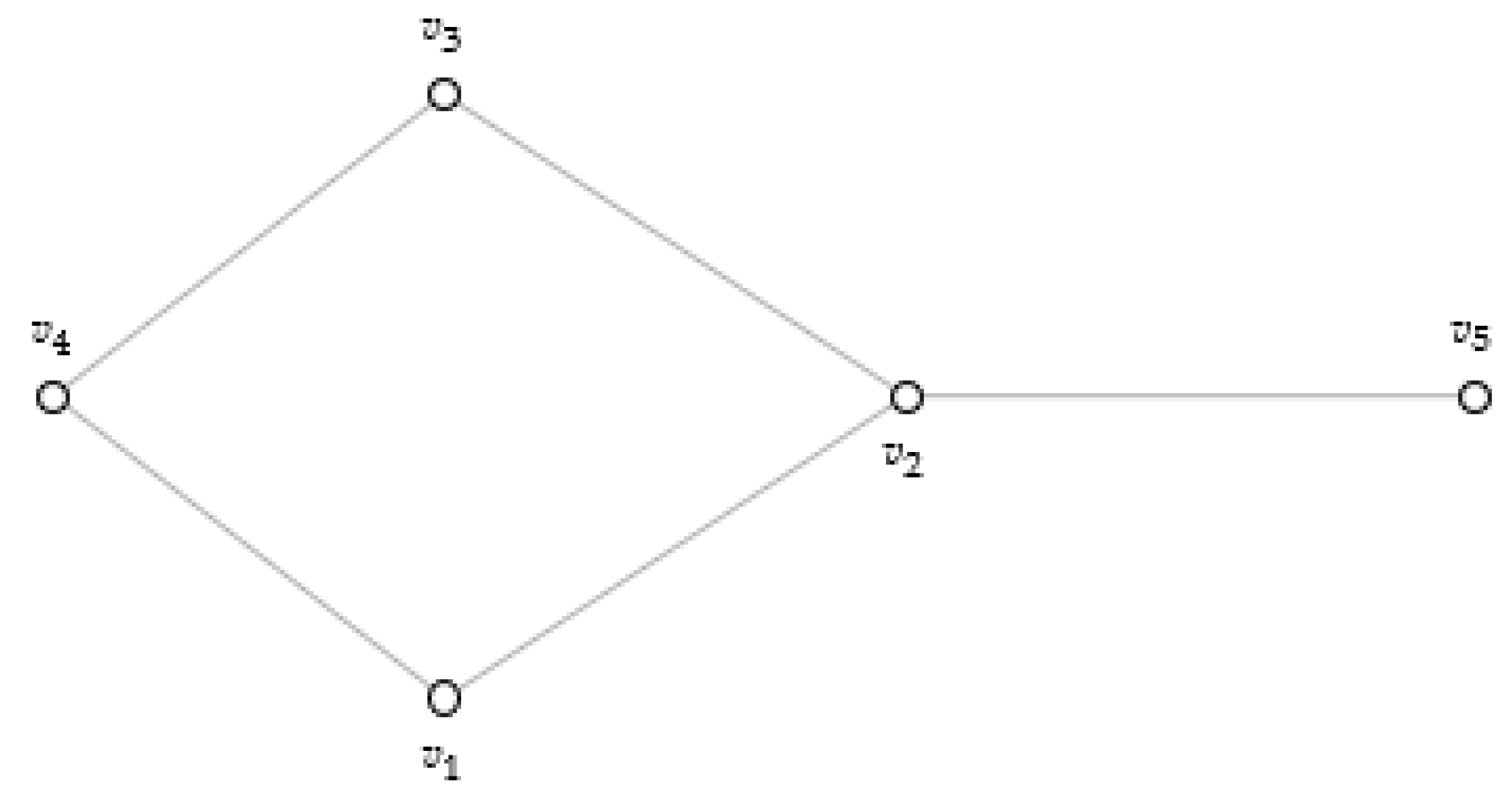
Example 1.

Let $G$ be a graph as shown in Figure 1, the $S_j$-neighborhoods of $v$, $j\in J$ are obtained as follows:

For $j\in \left\{r,l,u,i\right\}$; $S_j\left(v_1\right)=S_j\left(v_3\right)=\left\{v_1,v_3\right\}$, $S_j\left(v_2\right)=\left\{v_2\right\}$, $S_j\left(v_4\right)=\left\{v_2,v_4\right\}$, $S_j\left(v_5\right)=\left\{v_1,v_3,v_5\right\}$. For $j\in \left\{〈r〉,〈l〉,〈u〉,〈i〉\right\}$, $S_j\left(v_1\right)=S_j\left(v_3\right)=\left\{v_1,v_3,v_5\right\}$, $S_j\left(v_2\right)=\left\{v_2,v_4\right\}$, $S_j\left(v_4\right)=\left\{v_4\right\}$, $S_j\left(v_5\right)=\left\{v_5\right\}$.

Definition 12.

Let $G=\left(V,E\right)$ be a graph and $H=\left(V\left(H\right),E\left(H\right)\right)$ be a subgraph of $G$ and $I$ be an ideal on $G$. For $j\in J$, then $I_{S_j}$-lower approximations and $I_{S_j}$-upper approximations are defined by:

(a) 

${\underset{\_}{S}}_j^I\left(V\left(H\right)\right)=\left\{v\in V:S_j\left(v\right)\cap V{\left(H\right)}^{ı}\in I\right\}$;

(b) 

${\overline{S}}_j^I\left(V\left(H\right)\right)=V\left(H\right)\cup \left\{v\in V:S_j\left(v\right)\cap V\left(H\right)\notin I\right\}$.

Proposition 2.

Let $G=\left(V,E\right)$ be a graph and $H=\left(V\left(H\right),E\left(H\right)\right)$ be a subgraph of $G$ and $I$ be an ideal on $G$. Then for every $j\in J$, the following relationships hold:

(a) 

$V\left(M\right)\subseteq {\overline{S}}_j^I\left(V\left(M\right)\right)$;

(b) 

$V\left(M\right)\subseteq V\left(N\right)$ implies ${\underset{\_}{S}}_j^I\left(V\left(M\right)\right)\subseteq {\underset{\_}{S}}_j^I\left(V\left(N\right)\right)$;

$V\left(M\right)\subseteq V\left(N\right)$ implies ${\overline{S}}_j^I\left(V\left(M\right)\right)\subseteq {\overline{S}}_j^I\left(V\left(N\right)\right)$;

(c) 

${\underset{\_}{S}}_j^I\left(V\right)={\overline{S}}_j^I\left(V\right)=V$;

${\overline{S}}_j^I(\varnothing )=\varnothing$;

(d) 

${\underset{\_}{S}}_j^I\left(V\left(M\right)\cup V\left(N\right)\right)\supseteq {\underset{\_}{S}}_j^I\left(V\left(M\right)\right)\cup {\underset{\_}{S}}_j^I\left(V\left(N\right)\right)$;

${\overline{S}}_j^I\left(V\left(M\right)\cup V\left(N\right)\right)={\overline{S}}_j^I\left(V\left(M\right)\right)\cup {\overline{S}}_j^I\left(V\left(N\right)\right)$;

(e) 

${\underset{\_}{S}}_j^I\left(V\left(M\right)\cap V\left(N\right)\right)={\underset{\_}{S}}_j^I\left(V\left(M\right)\right)\cap {\underset{\_}{S}}_j^I\left(V\left(N\right)\right)$;

${\overline{S}}_j^I\left(V\left(M\right)\cap V\left(N\right)\right)\subseteq {\overline{S}}_j^I\left(V\left(M\right)\right)\cap {\overline{S}}_j^I\left(V\left(N\right)\right)$;

(f) 

If $V{\left(M\right)}^{ı}\in I$ then ${\underset{\_}{S}}_j^I\left(V\left(M\right)\right)=V$;

If $V\left(M\right)\in I$ then ${\overline{S}}_j^I\left(V\left(M\right)\right)=V\left(M\right)$.

Proof. 

It is adequate to prove $\left(\mathrm{a}\right)$ and (e). The other details are obvious from Definition 12 and the definition of an ideal.

(a) Let v $\in {\underset{\_}{S}}_j^I\left(\mathrm{V}\left(\mathrm{M}\right)\right)$. Then $S_j\left(v\right)\cap V{\left(M\right)}^{ı}\in I$. Since $V\left(M\right)\subseteq V\left(N\right)$, following the concept of the ideal, $S_j\left(v\right)\cap \mathrm{V}{\left(\mathrm{N}\right)}^{ı}\in I$. Hence ${\underset{\_}{S}}_j^I\left(\mathrm{V}\left(\mathrm{M}\right)\right)\subseteq {\underset{\_}{S}}_j^I\left(\mathrm{V}\left(\mathrm{N}\right)\right)$.

(e) We obtain ${\underset{\_}{S}}_j^I\left(\mathrm{V}\left(\mathrm{M}\right)\cap \mathrm{V}\left(\mathrm{N}\right)\right)\subseteq {\underset{\_}{S}}_j^I\left(\mathrm{V}\left(\mathrm{M}\right)\right)\cap {\underset{\_}{S}}_j^I\left(\mathrm{V}\left(\mathrm{N}\right)\right)$ via (b). Let $v\in {\underset{\_}{S}}_j^I\left(\mathrm{V}\left(\mathrm{M}\right)\right)\cap {\underset{\_}{S}}_j^I\left(\mathrm{V}\left(\mathrm{N}\right)\right)$. So, $v\in {\underset{\_}{S}}_j^I\left(\mathrm{V}\left(\mathrm{M}\right)\right)$ and $v\in {\underset{\_}{S}}_j^I\left(\mathrm{V}\left(\mathrm{N}\right)\right)$. Based on the definition of the $I_{S_j}$-lower approximations, we find that $S_j\left(v\right)\cap V{\left(M\right)}^{ı}\in I$ and $S_j\left(v\right)\cap V{\left(N\right)}^{ı}\in I.$ According to the concept of the ideal, $v\in {\underset{\_}{S}}_j^I\left(\mathrm{V}\left(\mathrm{M}\right)\cap \mathrm{V}\left(\mathrm{N}\right)\right)$. Therefore, ${\underset{\_}{S}}_j^I\left(\mathrm{V}\left(\mathrm{M}\right)\right)\cap {\underset{\_}{S}}_j^I\left(\mathrm{V}\left(\mathrm{N}\right)\right)\subseteq {\underset{\_}{S}}_j^I\left(\mathrm{V}\left(\mathrm{M}\right)\cap \mathrm{V}\left(\mathrm{N}\right)\right)$. □

In general, the equations in Proposition 2 (d) and Proposition 2 (e) may not always be true as shown in the following example. Additionally, we show that the converse implications of Proposition 2 (b) and (f) may not hold.

Example 2.

Let $G$ be a graph as shown in Figure 1 and $I=\left\{\varnothing ,\left\{v_3\right\}\right\}$.

(a) 

Let $V\left(H\right)=\left\{v_1,v_4\right\}$ and $V\left(M\right)=\left\{v_2,v_5\right\}$, ${\underset{\_}{S}}_r^I\left(V\left(H\right)\cup V\left(M\right)\right)=V\left(G\right).$ ${\underset{\_}{S}}_r^I\left(V\left(H\right)\right)=\left\{v_1,v_3\right\}$ and ${\underset{\_}{S}}_r^I\left(V\left(M\right)\right)=\left\{v_2\right\}$. So ${\underset{\_}{S}}_r^I\left(V\left(H\right)\cup V\left(M\right)\right)\ne {\underset{\_}{S}}_r^I\left(V\left(H\right)\right)\cup {\underset{\_}{S}}_r^I\left(V\left(M\right)\right)$.

(b) 

Let $V\left(H\right)=\left\{v_1,v_4\right\}$ and $V\left(M\right)=\left\{v_1,v_5\right\}$. ${\underset{\_}{S}}_r^I\left(V\left(M\right)\right)=\left\{v_1,v_3,v_5\right\}$. We obtain ${\underset{\_}{S}}_r^I\left(V\left(H\right)\right)\subseteq {\underset{\_}{S}}_r^I\left(V\left(M\right)\right)$, but it is not $V\left(H\right)⊈V\left(M\right)$.

(c) 

Let $V\left(H\right)=\left\{v_1,v_4\right\}$ and $V\left(M\right)=\left\{v_2,v_5\right\}$, ${\overline{S}}_r^I\left(V\left(H\right)\cap V\left(M\right)\right)=\varnothing$. ${\overline{S}}_r^I\left(V\left(H\right)\right)=\left\{v_1,v_3,v_4,v_5\right\}$ and ${\overline{S}}_r^I\left(V\left(M\right)\right)=\left\{v_2,v_4,v_5\right\}$. Hence, ${\overline{S}}_r^I\left(V\left(H\right)\cap V\left(N\right)\right)\ne {\overline{S}}_r^I\left(V\left(H\right)\right)\cap {\overline{S}}_r^I\left(V\left(N\right)\right)$.

(d) 

Let $V\left(H\right)=\left\{v_1,v_2\right\}$. Then ${\overline{S}}_r^I\left(V\left(H\right)\right)=V\left(G\right)$ while $V\left(H\right)\notin I$.

Remark 1.

In Pawlak’s rough set model, the following properties that are given in Proposition 1 do not always hold:

(a) 

${\underset{\_}{S}}_j^I\left(V\left(M\right)\right)V\left(M\right)$;

(b) 

${\underset{\_}{S}}_j^I\left({\underset{\_}{S}}_j^I\left(V\left(M\right)\right)\right)={\underset{\_}{S}}_j^I\left(V\left(M\right)\right)$;

${\overline{S}}_j^I\left({\overline{S}}_j^I\left(V\left(M\right)\right)\right)={\overline{S}}_j^I\left(V\left(M\right)\right)$;

(c) 

${({\underset{\_}{S}}_j^I\left(V\left(M\right)\right))}^{ı}={\overline{S}}_j^I\left(V{\left(M\right)}^{ı}\right)$;

${({\overline{S}}_j^I\left(V\left(M\right)\right))}^{ı}$ = ${\underset{\_}{S}}_j^I$($V{\left(M\right)}^{ı}$).

Example 3.

(a) 

Let $G$ be a graph as shown in Figure 1 and $I=\left\{\varnothing ,\left\{v_3\right\}\right\}$.

i. 

Let $V\left(M\right)=\left\{v_1,v_4\right\}$. Then ${\underset{\_}{S}}_r^I\left(V\left(M\right)\right)=\left\{v_1,v_3\right\}$. So ${\underset{\_}{S}}_r^I\left(V\left(M\right)\right)⊈V\left(M\right)$.

ii. 

Let $V\left(M\right)=\left\{v_2,v_3,v_4\right\}$. Then ${\overline{S}}_r^I\left(V\left(M\right)\right)=\left\{v_2,v_3,v_4\right\}$ and ${\underset{\_}{S}}_r^I\left(V{\left(M\right)}^{ı}\right))=\left\{v_1,v_3,v_5\right\}$. Hence, ${({\underset{\_}{S}}_r^I\left(V\left(M\right)\right))}^{ı}\ne {\overline{S}}_r^I$($V{\left(M\right)}^{ı}$).

(b) 

Let $G$ be a graph as shown in Figure 2 and $I=\left\{\varnothing ,\left\{v_2\right\},\left\{v_3\right\},\left\{v_2,v_3\right\}\right\}$. Let $V\left(M\right)=\left\{v_4\right\}$. Then ${\overline{S}}_r^I\left(V\left(M\right)\right)=\left\{v_1,v_4,v_5\right\}$ and ${\overline{S}}_r^I\left({\overline{S}}_r^I\left(V\left(M\right)\right)\right)=V\left(G\right)$. Hence ${\overline{S}}_r^I\left({\overline{S}}_r^I\left(V\left(M\right)\right)\right)\ne$ ${\overline{S}}_r^I\left(V\left(M\right)\right).$

The proposition below is the comparison of the given lower approximations.

Proposition 3.

The following properties always hold:

(a) 

${\underset{\_}{S}}_u^I\left(V\left(M\right)\right)\subseteq {\underset{\_}{S}}_r^I\left(V\left(M\right)\right)\subseteq {\underset{\_}{S}}_i^I\left(V\left(M\right)\right)$;

(b) 

${\underset{\_}{S}}_u^I\left(V\left(M\right)\right)\subseteq {\underset{\_}{S}}_l^I\left(V\left(M\right)\right)\subseteq {\underset{\_}{S}}_i^I\left(V\left(M\right)\right)$;

(c) 

;

(d) 

.

Proof. 

The proof of Proposition 3 is straightforward. □

The proposition below is the comparison of the given upper approximations.

Proposition 4.

The following properties always hold:

(a) 

${\overline{S}}_u^I\left(V\left(H\right)\right)\subseteq {\overline{S}}_r^I\left(V\left(H\right)\right)\subseteq {\overline{S}}_i^I\left(V\left(H\right)\right)$;

(b) 

${\overline{S}}_u^I\left(V\left(H\right)\right)\subseteq {\overline{S}}_l^I\left(V\left(H\right)\right)\subseteq {\overline{S}}_i^I\left(V\left(H\right)\right)$;

(c) 

;

(d) 

.

Proof. 

The proof of Proposition 4 is straightforward. □

Lemma 1.

Let $G$ be a graph, $H$ a subgraph of $G$ and $I$, $\mathcal{J}$ two ideals on $G$. If $I\subseteq \mathcal{J}$, the following properties hold:

(a) 

${\underset{\_}{S}}_j^I\left(V\left(H\right)\right)\subseteq {\underset{\_}{S}}_j^{\mathcal{J}}\left(V\left(H\right)\right)$;

(b) 

${\overline{S}}_j^{\mathcal{J}}\left(V\left(H\right)\right)\subseteq {\overline{S}}_j^I\left(V\left(H\right)\right)$.

Proof. 

(a)

Let $v\in$ ${\underset{\_}{S}}_j^I\left(V\left(H\right)\right).$ Then $S_j\left(v\right)\cap V{\left(H\right)}^{ı}\in I$. Since $I\subseteq \mathcal{J},$ we have $S_j\left(v\right)\cap V{\left(H\right)}^{ı}\in \mathcal{J}.$ Hence, we obtain $\in$ ${\underset{\_}{S}}_j^J\left(V\left(H\right)\right)$.

(b)

The proof is similar to (a).

 □

We formulate new approximations as $I_{S_j^{*}}$-lower approximations and $I_{S_j^{*}}$-upper approximations by using ideals and the $S_j$-neighborhood.

Definition 13.

Let $G$ be a graph, $H$ a subgraph of $G$ and $I$ an ideal on $G$. For every $j\in J$, $I_{S_j^{*}}$-lower approximations and $I_{S_j^{*}}$-upper approximations are defined by:

(a) 

${\underset{\_}{S}}_j^{*I}\left(V\left(H\right)\right)=V\left(H\right)\cap {\underset{\_}{S}}_j^I\left(V\left(H\right)\right)$;

(b) 

${\overline{S}}_j^{*I}\left(V\left(H\right)\right)=V\left(H\right)\cup {\overline{S}}_j^I\left(V\left(H\right)\right)$.

In Proposition 5, in addition to the properties mentioned in Proposition 2, the properties (L6–7) and (U6–7) in Pawlak’s rough set model are also provided by Definition 13.

Proposition 5.

Let $G$ be a graph, $H$ a subgraph of $G$ and $I$ an ideal on $G$. For every $j\in J$, the following properties apply:

(a) 

${\underset{\_}{S}}_j^{*I}\left(V\left(H\right)\right)\subseteq V\left(H\right)\subseteq {\overline{S}}_j^{*I}\left(V\left(H\right)\right)$;

(b) 

${\overline{S}}_j^{*I}\left(\varnothing \right)={\underset{\_}{S}}_j^{*I}\left(\varnothing \right)=\varnothing .$

Proof. 

The proof is obvious from Definition 13. □

In the following definition, the concept of the ideal and Definition 13 are used to introduce the new concepts of $I_{S_j^{*}}$-boundary regions and $I_{S_j^{*}}$-accuracy measures.

Definition 14.

Let $G$ be a graph, $H$ a subgraph of $G$ and $I$ an ideal on $G$. For every $j\in J$, $I_{S_j{}^{*}}$-boundary regions and $I_{S_j{}^{*}}$-accuarcy of approximations of $V\left(H\right)$ are defined by:

(a) 

$B_{S_j^{*}}^I\left(V\left(H\right)\right)={\overline{S}}_j^{*I}\left(V\left(H\right)\right)-{\underset{\_}{S}}_j^{*I}\left(V\left(H\right)\right)$;

(b) 

${\sigma }_{N_j^{*}}^I\left(V\left(H\right)\right)=\frac{\left|{\underset{\_}{S}}_j^{*I}\left(V\left(H\right)\right)\right|}{\left|{\overline{S}}_j^{*I}\left(V\left(H\right)\right)\right|}$, where $\left|{\overline{S}}_j^{*I}\left(V\left(H\right)\right)\right|\ne \varnothing$.

Corollary 1.

The following properties always hold:

(a) 

$B_{S_u}^I\left(V\left(M\right)\right)\subseteq B_{S_r}^I\left(V\left(M\right)\right)\subseteq B_{S_i}^I\left(V\left(M\right)\right)$;

(b) 

$B_{S_u}^I\left(V\left(M\right)\right)\subseteq B_{S_r}^I\left(V\left(M\right)\right)\subseteq B_{S_i}^I\left(V\left(M\right)\right)$;

(c) 

;

(d) 

.

Proof. 

The proof is obvious from Definition 14 and Propositions 3 and 4. □

Corollary 2.

The following properties always hold:

(a) 

${\sigma }_{S_u}^I\left(V\left(M\right)\right)\le {\sigma }_{S_r}^I\left(V\left(M\right)\right)\le {\sigma }_{S_i}^I\left(V\left(M\right)\right)$;

(b) 

${\sigma }_{S_u}^I\left(V\left(M\right)\right)\le {\sigma }_{S_r}^I\left(V\left(M\right)\right)\le {\sigma }_{S_i}^I\left(V\left(M\right)\right)$;

(c) 

;

(d) 

.

Proof. 

The proof is obvious from Definition 14 and Propositions 3 and 4. □

Definition 15.

For every $j\in J$, a subgraph $M$ is called $H_{S_j^I}$-definable ($H_{S_j^I}$-exact) if ${\overline{S}}_j^{*I}\left(V\left(M\right)\right)={\underset{\_}{S}}_j^{*I}\left(V\left(M\right)\right)$. Otherwise, $M$ is called $H_{S_j^I}$-rough set.

Lemma 2.

Let $G$ be a graph, $M$ a subgraph of $G$ and $I$ an ideal on $G$. For every $j\in J$, $M$ is $H_{S_j^I}$-exact if $B_{S_j^{*}}^I\left(V\left(M\right)\right)=\varnothing$.

Example 4.

Let $G$ be a graph as shown in Figure 1 and $I=\left\{\varnothing ,\left\{v_1\right\},\left\{v_3\right\},\left\{v_1,v_3\right\}\right\}$. Let $V\left(M\right)=\left\{v_1,v_2,v_4,v_5\right\}$. Then, $M$ is $H_{S_j^I}$-exact.

4. Brief Account of the $\mathit{I}$-C-$\mathit{j}$ Approximations

In this section we generalize Definition 3.1 from [6] in terms of containment neighborhoods, which are introduced in Definition 16. We report the lower and upper approximations by using the concepts of containment neighborhoods and the ideal.

Definition 16.

Let $G=\left(V,E\right)$ be a graph. For each $v\in V$, the $C_j$-neighborhood of $v$, $j\in J$ is defined as [6]:

(a) 

$C_r\left(v\right)=\left\{w\in V:N_r\left(w\right)\subseteq N_r\left(v\right)\right\}$;

(b) 

$C_l\left(v\right)=\left\{w\in V:N_l\left(w\right)\subseteq N_l\left(v\right)\right\}$;

(c) 

$C_u\left(v\right)=C_r\left(v\right)\cup C_l\left(v\right)$;

(d) 

$C_i\left(v\right)=C_r\left(v\right)\cap C_l\left(v\right)$;

(e) 

;

(f) 

;

(g) 

;

(h) 

.

Definition 17.

Let $G$ be a graph, $H$ a subgraph of $G$ and $I$ an ideal on $G$. For $j\in J$, the $I_{C_j}$-lower approximations and $I_{C_j}$-upper approximations are defined by the following:

(a) 

${\underset{\_}{C}}_j^I\left(V\left(H\right)\right)=\left\{v\in V:C_j\left(v\right)\cap V{\left(H\right)}^{ı}\in I\right\}$;

(b) 

${\overline{C}}_j^I\left(V\left(H\right)\right)=V\left(H\right)\cup \left\{v\in V:C\left(v\right)\cap V\left(H\right)\notin I\right\}$.

Proposition 6.

Let $G=\left(V,E\right)$ be a graph, $Mand$ $N$ be subgraphs of $G$ and $I$ an ideal on $G$. For every $j\in J$, the following properties hold:

(a) 

$V\left(M\right)\subseteq {\overline{C}}_j^I\left(V\left(M\right)\right)$;

(b) 

$V\left(M\right)\subseteq V\left(N\right)$ implies ${\underset{\_}{C}}_j^I\left(V\left(M\right)\right)\subseteq {\underset{\_}{C}}_j^I\left(V\left(N\right)\right)$;

$V\left(M\right)\subseteq V\left(N\right)$ implies ${\overline{C}}_j^I\left(V\left(M\right)\right)\subseteq {\overline{C}}_j^I\left(V\left(N\right)\right)$;

(c) 

${\underset{\_}{C}}_j^I\left(V\right)={\overline{C}}_j^I\left(V\right)=V$;

${\overline{C}}_j^I\left(\varnothing \right)=\varnothing$;

(d) 

$C_j^I\left(V\left(M\right)\cup V\left(N\right)\right)\supseteq {\underset{\_}{C}}_j^I\left(V\left(M\right)\right)\cup {\underset{\_}{C}}_j^I\left(V\left(N\right)\right)$;

${\overline{C}}_j^I\left(V\left(M\right)\cup V\left(N\right)\right)={\overline{C}}_j^I\left(V\left(M\right)\right)\cup {\overline{C}}_j^I\left(V\left(N\right)\right)$;

(e) 

$C_j^I\left(V\left(M\right)\cap V\left(N\right)\right)={\underset{\_}{C}}_j^I\left(V\left(M\right)\right)\cap {\underset{\_}{C}}_j^I\left(V\left(N\right)\right)$;

${\overline{C}}_j^I\left(V\left(M\right)\cap V\left(N\right)\right)\subseteq {\overline{C}}_j^I\left(V\left(M\right)\right)\cap {\overline{C}}_j^I\left(V\left(N\right)\right)$;

(f) 

If $V{\left(M\right)}^{ı}\in I$ then ${\underset{\_}{C}}_j^I\left(V\left(M\right)\right)=V$;

If $V\left(M\right)\in I$ then ${\overline{C}}_j^I\left(V\left(M\right)\right)=V\left(M\right)$.

Proof. 

The proof for Proposition 6 is similar to the one provided for Proposition 2. □

In general, the equations in Proposition 6 (d) and Proposition 6 (e) may not always be true as shown in the following example. Additionally, we show that the converse implications of Proposition 6 (b) and (f) may not hold.

Example 5.

Let $G$ be a graph as shown in Figure 1 and $I=\left\{\varnothing ,\left\{v_2\right\},\left\{v_3\right\},\left\{v_2,v_3\right\}\right\}$.

(a) 

Let $V\left(H\right)=\left\{v_1,v_4\right\}$ and $V\left(M\right)=\left\{v_2,v_5\right\},$ and let ${\underset{\_}{C}}_r^I\left(V\left(H\right)\cup V\left(M\right)\right)=V$. ${\underset{\_}{C}}_r^I\left(V\left(H\right)\right)=\left\{v_2,v_4\right\}$ and ${\underset{\_}{C}}_r^I\left(V\left(M\right)\right)=\left\{v_5\right\}$. Hence, ${\underset{\_}{C}}_r^I\left(V\left(H\right)\cup V\left(M\right)\right)\ne C_r^I\left(V\left(H\right)\right)\cup {\underset{\_}{C}}_r^I\left(V\left(M\right)\right)$.

(b) 

Let $V\left(H\right)=\left\{v_2,v_5\right\}$ and $V\left(M\right)=\left\{v_4,v_5\right\}$. ${\underset{\_}{C}}_r^I\left(V\left(M\right)\right)=\left\{v_2,v_4,v_5\right\}$. We obtain ${\underset{\_}{C}}_r^I\left(V\left(H\right)\right)\subseteq {\underset{\_}{C}}_r^I\left(V\left(M\right)\right)$, but it is not $V\left(H\right)⊈V\left(M\right)$.

(c) 

Let $V\left(H\right)=\left\{v_1,v_4\right\}$ and $V\left(M\right)=\left\{v_2,v_5\right\}$, and let ${\overline{C}}_r^I\left(V\left(H\right)\cap V\left(M\right)\right)=\varnothing$. ${\overline{C}}_r^I\left(V\left(H\right)\right)=\left\{v_1,v_2,v_3,v_4\right\}$ and ${\overline{C}}_r^I\left(V\left(M\right)\right)=\left\{v_1,v_2,v_3,v_5\right\}$. Hence, ${\overline{C}}_r^I\left(V\left(H\right)\cap V\left(M\right)\right)\ne {\overline{C}}_r^I\left(V\left(H\right)\right)\cap {\overline{C}}_r^I\left(V\left(M\right)\right)$.

(d) 

Let $V\left(H\right)=\left\{v_1,v_3\right\}$. It follows that ${\overline{C}}_r^I\left(V\left(H\right)\right)=V\left(H\right)$ while $V\left(H\right)\notin I$.

Remark 2.

In Pawlak’s rough set model, the following properties that are given in Proposition 6 do not always hold:

(a) 

${\underset{\_}{C}}_j^I\left(V\left(M\right)\right)\subseteq V\left(M\right)$;

(b) 

${\underset{\_}{C}}_j^I\left({\underset{\_}{C}}_j^I\left(V\left(M\right)\right)\right)={\underset{\_}{C}}_j^I\left(V\left(M\right)\right);$

${\overline{C}}_j^I\left({\overline{C}}_j^I\left(V\left(M\right)\right)\right)={\overline{C}}_j^I\left(V\left(M\right)\right)$;

(c) 

${({\underset{\_}{C}}_j^I\left(V\left(M\right)\right))}^{ı}={\overline{C}}_j^I\left(V{\left(M\right)}^{ı}\right)$.

Example 6.

Let $G$ be a graph as shown in Figure 1 and $I=\left\{\varnothing ,\left\{v_2\right\},\left\{v_3\right\},\left\{v_2,v_3\right\}\right\}.$

(a) 

Let $V\left(M\right)=\left\{v_1,v_4\right\}$. Then, ${\underset{\_}{C}}_r^I\left(V\left(M\right)\right)=\left\{v_2,v_4\right\}$. Hence, ${\underset{\_}{C}}_r^I\left(V\left(M\right)\right)⊈V\left(M\right)$.

(b) 

Let $V\left(M\right)=\left\{v_2,v_5\right\}$. Then ${\overline{C}}_r^I\left(V\left(M\right)\right)=\left\{v_1,v_2,v_3,v_5\right\}$ and ${\overline{C}}_j^I\left({\overline{C}}_j^I\left(V\left(M\right)\right)\right)=V$. Hence, ${\overline{C}}_j^I\left({\overline{C}}_j^I\left(V\left(M\right)\right)\right)\ne {\overline{C}}_j^I\left(V\left(M\right)\right)$.

(c) 

Let $V\left(M\right)=\left\{v_1,v_4\right\}$. Then, ${\underset{\_}{C}}_r^I\left(V\left(M\right)\right)=\left\{v_2,v_4\right\}$ and ${\overline{C}}_j^I\left(V{\left(M\right)}^{ı}\right)=\left\{v_2,v_3,v_5\right\}$. Hence, ${({\underset{\_}{C}}_j^I\left(V\left(M\right)\right))}^{ı}\ne {\overline{C}}_j^I$($V{\left(M\right)}^{ı}$).

The proposition below is the comparison of the given upper approximations.

Proposition 7.

The following properties always hold:

(a) 

${\underset{\_}{C}}_u^I\left(V\left(M\right)\right)\subseteq {\underset{\_}{C}}_r^I\left(V\left(M\right)\right)\subseteq {\underset{\_}{C}}_i^I\left(V\left(M\right)\right)$;

(b) 

${\underset{\_}{C}}_u^I\left(V\left(M\right)\right)\subseteq {\underset{\_}{C}}_l^I\left(V\left(M\right)\right)\subseteq {\underset{\_}{C}}_i^I\left(V\left(M\right)\right)$;

(c) 

;

(d) 

.

Proof. 

The proof of Proposition 7 is straightforward. □

The proposition below is the comparison of the given upper approximations.

Proposition 8.

The following properties always hold:

(a) 

${\overline{C}}_u^I\left(V\left(M\right)\right)\subseteq {\overline{C}}_r^I\left(V\left(M\right)\right)\subseteq {\overline{C}}_i^I\left(V\left(M\right)\right)$;

(b) 

${\overline{C}}_u^I\left(V\left(M\right)\right)\subseteq {\overline{C}}_l^I\left(V\left(M\right)\right)\subseteq {\overline{C}}_i^I\left(V\left(M\right)\right)$;

(c) 

;

(d) 

.

Proof. 

The proof of Proposition 8 is straightforward. □

Lemma 3.

Let $G$ be a graph, $M$ a subgraph of $G$ and $I,\mathcal{J}$ ideals on $G$. If $I\subseteq \mathcal{J}$, the following properties hold:

(a) 

${\underset{\_}{C}}_j^I\left(V\left(M\right)\right)\subseteq {\underset{\_}{C}}_j^{\mathcal{J}}\left(V\left(M\right)\right)$;

(b) 

${\overline{C}}_j^{\mathcal{J}}\left(V\left(M\right)\right)\subseteq {\overline{C}}_j^I\left(V\left(M\right)\right)$.

Proof. 

The proof for Lemma 3 is similar to the one provided for Lemma 1. □

We formulate new approximations as $I_{C_j^{*}}$-lower approximations and $I_{C_j^{*}}$-upper approximations by using ideals and $C_j$-neighborhood.

Definition 18.

Let $G$ be a graph, $H$ a subgraph of $G$ and $I$ an ideal on $G$. In this context, for every $j\in J$, $I_{C_j^{*}}$-lower approximations and $I_{C_j^{*}}$-upper approximations are defined by the following:

(a) 

${\underset{\_}{C}}_j^{*I}\left(V\left(H\right)\right)=V\left(H\right)\cap {\underset{\_}{C}}_j^I\left(V\left(H\right)\right)$;

(b) 

${\overline{C}}_j^{*I}\left(V\left(H\right)\right)=V\left(H\right)\cup {\overline{C}}_j^I\left(V\left(H\right)\right)$.

In Proposition 9, in addition to the properties from Proposition 6, the properties (L6–7), (U6–7) in Pawlak’s rough set model are also provided through Definition 18.

Proposition 9.

Let $G$ be a graph, $H$ a subgraph of $G$ and $I$ an ideal on $G$. Hence, for every $j\in J$, the following properties apply:

(a) 

${\underset{\_}{C}}_j^{*I}\left(V\left(H\right)\right)\subseteq V\left(H\right)\subseteq {\overline{C}}_j^{*I}\left(V\left(H\right)\right)$;

(b) 

${\overline{C}}_j^{*I}\left(\varnothing \right)={\underset{\_}{C}}_j^{*I}\left(\varnothing \right)=\varnothing$.

In the following definition, the information from Definition 18 is used to introduce the new concepts of $I_{C_j^{*}}$-boundary regions and $I_{C_j^{*}}$-accuracy measures.

Definition 19.

Let $G$ be a graph, $H$ be a subgraph of $G$ and $I$ an ideal on $G$. Then, for every $j\in J$, $I_{C_j{}^{*}}$-boundary regions and $I_{C_j{}^{*}}$-accuarcy of approximations of $V\left(H\right)$ are defined as follows:

(a) 

$B_{C_j^{*}}^I\left(V\left(H\right)\right)={\overline{C}}_j^{*I}\left(V\left(H\right)\right)-{\underset{\_}{C}}_j^{*I}\left(V\left(H\right)\right)$;

(b) 

${\sigma }_{C_j^{*}}^I\left(V\left(H\right)\right)=\frac{\left|{\underset{\_}{C}}_j^{*I}\left(V\left(H\right)\right)\right|}{\left|{\overline{C}}_j^{*I}\left(V\left(H\right)\right)\right|}$ where $\left|{\overline{C}}_j^{*I}\left(V\left(H\right)\right)\right|\ne \varnothing$.

Definition 20.

For every $j\in J$, the subgraph $H$ is called $H_{C_j^I}$-definable ($H_{C_j^I}$-exact) if ${\overline{C}}_j^{*I}\left(V\left(M\right)\right)={\underset{\_}{C}}_j^{*I}\left(V\left(M\right)\right)$. Otherwise, $H$ is called $H_{C_j^I}$-rough set.

Lemma 4.

Let $G$ be a graph, $M$ be a subgraph of $G$ and $I$ an ideal on $G$. In this case, for every $j\in J$, M is $H_{C_j^I}$-exact iff $B_{C_j^{*}}^I\left(V\left(M\right)\right)=\varnothing$.

Example 7.

Let $G$ be a graph as shown in Figure 2 and $I=\left\{\varnothing ,\left\{v_2\right\},\left\{v_5\right\},\left\{v_2,v_5\right\}\right\}$. Let $V\left(M\right)=\left\{v_1,v_2,v_4,v_5\right\}$. Then, $M$ is $H_{C_j^I}$-exact.

Corollary 3.

The following properties always hold:

(a) 

$B_{C_u}^I\left(V\left(M\right)\right)\subseteq B_{C_r}^I\left(V\left(M\right)\right)\subseteq B_{C_i}^I\left(V\left(M\right)\right)$;

(b) 

$B_{C_u}^I\left(V\left(M\right)\right)\subseteq B_{C_l}^I\left(V\left(M\right)\right)\subseteq B_{C_i}^I\left(V\left(M\right)\right)$;

(c) 

;

(d) 

.

Proof. 

The proof is obvious from Definition 19 and Propositions 7 and 8. □

Corollary 4.

The following properties always hold:

(a) 

${\sigma }_{C_u}^I\left(V\left(M\right)\right)\le {\sigma }_{C_r}^I\left(V\left(M\right)\right)\le {\sigma }_{C_i}^I\left(V\left(M\right)\right)$;

(b) 

${\sigma }_{C_u}^I\left(V\left(M\right)\right)\le {\sigma }_{C_l}^I\left(V\left(M\right)\right)\le {\sigma }_{C_i}^I\left(V\left(M\right)\right)$;

(c) 

;

(d) 

.

Proof. 

The proof is obvious from Definition 19 and Propositions 7 and 8. □

Remark 3.

(a) 

The boundary regions and accuracy measures in

Table A1. Comparison between the $j$-boundary and $j$-accuracy measures by using our approach for $j=\left\{r,l,u,i\right\}$.

$\mathit{V}\left(\mathit{H}\right)$	$\mathbf{For}\mathit{j}=\mathit{r}$		$\mathbf{For}\mathit{j}=\mathit{l}$		$\mathbf{For}\mathit{j}=\mathit{u}$		$\mathbf{For}\mathit{j}=\mathit{i}$
	${\mathit{B}}_{{\mathit{S}}_{\mathit{r}}^{*}}^{\mathit{I}}\left(\mathbf{V}\left(\mathbf{H}\right)\right)$	${\mathit{\sigma }}_{{\mathit{S}}_{\mathit{r}}^{*}}^{\mathit{I}}\left(\mathbf{V}\left(\mathbf{H}\right)\right)$	${\mathit{B}}_{{\mathit{S}}_{\mathit{l}}^{*}}^{\mathit{I}}\left(\mathbf{V}\left(\mathbf{H}\right)\right)$	${\mathit{\sigma }}_{{\mathit{S}}_{\mathit{l}}^{*}}^{\mathit{I}}\left(\mathbf{V}\left(\mathbf{H}\right)\right)$	${\mathit{B}}_{{\mathit{S}}_{\mathit{u}}^{*}}^{\mathit{I}}\left(\mathbf{V}\left(\mathbf{H}\right)\right)$	${\mathit{\sigma }}_{{\mathit{S}}_{\mathit{u}}^{*}}^{\mathit{I}}\left(\mathbf{V}\left(\mathbf{H}\right)\right)$	${\mathit{B}}_{{\mathit{S}}_{\mathit{i}}^{*}}^{\mathit{I}}\left(\mathbf{V}\left(\mathbf{H}\right)\right)$	${\mathit{\sigma }}_{{\mathit{S}}_{\mathit{i}}^{*}}^{\mathit{I}}\left(\mathbf{V}\left(\mathbf{H}\right)\right)$
$\left\{v_1\right\}$	$\left\{v_1,v_4,v_5\right\}$	$0$	$\left\{v_1,v_4,v_5\right\}$	$0$	$\left\{v_1,v_4,v_5\right\}$	0	{v1}	$1/2$
{v2}	$\varnothing$	$1$	$\varnothing$	$1$	$\varnothing$	1	$\varnothing$	1
{v3}	$\varnothing$	1	$\varnothing$	1	$\varnothing$	1	$\varnothing$	1
{v4}	$\left\{v_1,v_4,v_5\right\}$	0	$\left\{v_4,v_5\right\}$	0	$\left\{v_1,v_4,v_5\right\}$	0	$\left\{v_4,v_5\right\}$	0
{v5}	{v5}	0	$\left\{v_4,v_5\right\}$	0	$\left\{v_4,v_5\right\}$	0	$\left\{v_4,v_5\right\}$	0
$\left\{v_1,v_2\right\}$	$\left\{v_1,v_4,v_5\right\}$	$1/4$	$\left\{v_5\right\}$	$1/3$	$\left\{v_4,v_5\right\}$	$1/2$	$\left\{v_4,v_5\right\}$	$1/2$
$\left\{v_1,v_3\right\}$	$\left\{v_1,v_4,v_5\right\}$	$1/4$	$\left\{v_4,v_5\right\}$	$1/2$	$\left\{v_1,v_4,v_5\right\}$	$1/4$	$\left\{v_4,v_5\right\}$	$1/2$
$\left\{v_1,v_4\right\}$	$\left\{v_1,v_4,v_5\right\}$	$0$	$\left\{v_4,v_5\right\}$	$1/3$	$\left\{v_1,v_4,v_5\right\}$	$0$	$\left\{v_4,v_5\right\}$	$1/3$
$\left\{v_1,v_5\right\}$	$\left\{v_1,v_2,v_4\right\}$	$1/4$	$\left\{v_4,v_5\right\}$	$1/3$	$\left\{v_1,v_2,v_4,v_5\right\}$	$0$	$\varnothing$	$1$
$\left\{v_2,v_3\right\}$	$\varnothing$	$1$	$\varnothing$	$1$	$\varnothing$	$1$	$\varnothing$	$1$
$\left\{v_2,v_4\right\}$	$\left\{v_1,v_2,v_4,v_5\right\}$	$1/4$	$\left\{v_4,v_5\right\}$	$1/3$	$\left\{v_1,v_2,v_4,v_5\right\}$	$1/4$	$\left\{v_4,v_5\right\}$	$1/3$
$\left\{v_2,v_5\right\}$	$\left\{v_5\right\}$	$1/2$	$\left\{v_4,v_5\right\}$	$1/3$	$\left\{v_4,v_5\right\}$	$1/3$	$\left\{v_5\right\}$	$1/2$
$\left\{v_3,v_4\right\}$	$\left\{v_1,v_4,v_5\right\}$	$1/4$	$\left\{v_4,v_5\right\}$	$1/3$	$\left\{v_1,v_4,v_5\right\}$	$1/4$	$\left\{v_5\right\}$	$1/2$
$\left\{v_3,v_5\right\}$	$\left\{v_5\right\}$	$1/2$	$\left\{v_4,v_5\right\}$	$1/3$	$\left\{v_4,v_5\right\}$	$1/3$	$\varnothing$	$1$
$\left\{v_4,v_5\right\}$	$\left\{v_1,v_4,v_5\right\}$	$0$	$\left\{v_4,v_5\right\}$	$0$	$\left\{v_1,v_2,v_4\right\}$	$0$	$\left\{v_4,v_5\right\}$	$0$
$\left\{v_1,v_2,v_3\right\}$	$\left\{v_1,v_4,v_5\right\}$	$3/5$	$\left\{v_4,v_5\right\}$	$3/5$	$\left\{v_4,v_5\right\}$	$3/5$	$\left\{v_4,v_5\right\}$	$3/5$
$\left\{v_1,v_2,v_4\right\}$	$\left\{v_5\right\}$	$3/4$	$\left\{v_4,v_5\right\}$	$1/2$	$\left\{v_1,v_4,v_5\right\}$	$1/4$	$\left\{v_4,v_5\right\}$	$1/2$
$\left\{v_1,v_2,v_5\right\}$	$\left\{v_1,v_4\right\}$	$1/2$	$\left\{v_4,v_5\right\}$	$1/2$	$\left\{v_1,v_4,v_5\right\}$	$1/4$	$\varnothing$	$1$
$\left\{v_1,v_3,v_4\right\}$	$\left\{v_4,v_5\right\}$	$1/2$	$\left\{v_4,v_5\right\}$	$1/2$	$\left\{v_4,v_5\right\}$	$1/2$	$\left\{v_4,v_5\right\}$	$1/2$
$\left\{v_1,v_3,v_5\right\}$	$\left\{v_1,v_4,v_5\right\}$	$1/4$	$\left\{v_1,v_4,v_5\right\}$	$1/4$	$\left\{v_1,v_4,v_5\right\}$	$1/4$	$\left\{v_1,v_4,v_5\right\}$	$1/4$
$\left\{v_1,v_4,v_5\right\}$	$\varnothing$	$1$	$\varnothing$	$1$	$\varnothing$	$1$	$\varnothing$	$1$
$\left\{v_2,v_3,v_4\right\}$	$\left\{v_1,v_4,v_5\right\}$	$2/5$	$\left\{v_4,v_5\right\}$	$1/2$	$\left\{v_1,v_4,v_5\right\}$	$2/5$	$\left\{v_4,v_5\right\}$	$1/2$
$\left\{v_2,v_3,v_5\right\}$	$\left\{v_5\right\}$	$2/3$	$\left\{v_4,v_5\right\}$	$1/2$	$\left\{v_4,v_5\right\}$	$1/2$	$\left\{v_5\right\}$	$2/3$
$\left\{v_2,v_4,v_5\right\}$	$\left\{v_1,v_4,v_5\right\}$	$1/4$	$\left\{v_4,v_5\right\}$	$1/3$	$\left\{v_1,v_4,v_5\right\}$	$1/4$	$\left\{v_4,v_5\right\}$	$1/3$
$\left\{v_3,v_4,v_5\right\}$	$\left\{v_1,v_4,v_5\right\}$	$1/4$	$\left\{v_4,v_5\right\}$	$1/3$	$\left\{v_1,v_4,v_5\right\}$	$1/4$	$\left\{v_4,v_5\right\}$	$1/3$
$\left\{v_1,v_2,v_3,v_4\right\}$	$\varnothing$	$1$	$\left\{v_4,v_5\right\}$	$2/5$	$\left\{v_4,v_5\right\}$	$2/5$	$\varnothing$	$1$
$\left\{v_1,v_2,v_3,v_5\right\}$	$\left\{v_1,v_4,v_5\right\}$	$2/5$	$\left\{v_4,v_5\right\}$	$3/5$	$\left\{v_1,v_4,v_5\right\}$	$2/5$	$\left\{v_4,v_5\right\}$	$3/5$
$\left\{v_1,v_2,v_4,v_5\right\}$	$\varnothing$	$1$	$\varnothing$	$1$	$\varnothing$	$1$	$\varnothing$	$1$
$\left\{v_2,v_3,v_4,v_5\right\}$	$\left\{v_1,v_4,v_5\right\}$	$2/5$	$\left\{v_4,v_5\right\}$	$1/2$	$\left\{v_1,v_4,v_5\right\}$	$2/5$	$\left\{v_4,v_5\right\}$	$1/2$

(see Appendix A) are generated using our method in accordance with Example 7, which assumes the ideal $I=\left\{\varnothing ,\left\{v_2\right\},\left\{v_3\right\},\left\{v_2,v_3\right\}\right\}$. Thus, it was noticed that $I_{S_i{}^{*}}$-accuracy is more precise than $I_{S_j{}^{*}}$-accuracy for $j=\left\{r,l,u\right\}$.

(b) 

The lower approximations, upper approximations, boundary regions and accuracy measures in

Table A2. Comparison between the lower approximations, upper approximations, $j$-boundary and $j$-accuracy measures by using Güler’s approach [28] and our approach for $j=l$.

$\mathit{V}\left(\mathit{H}\right)$	Güler’s Approach				Our Approach
	${\underset{¯}{\mathit{N}}}_{\mathit{l}\mathit{l}}^{*\mathit{I}}\left(\mathbf{V}\left(\mathbf{H}\right)\right)$	${\overline{\mathit{N}}}_{\mathit{l}\mathit{l}}^{*\mathit{I}}\left(\mathbf{V}\left(\mathbf{H}\right)\right)$	${\mathit{B}}_{\mathit{l}}^{*\mathit{I}}\left(\mathbf{V}\left(\mathbf{H}\right)\right)$	${\mathit{\sigma }}_{{\mathit{N}}_{\mathit{l}}}^{*\mathit{I}}\left(\mathbf{V}\left(\mathbf{H}\right)\right)$	${\underset{¯}{\mathit{C}}}_{\mathit{l}\mathit{l}}^{*\mathit{I}}\left(\mathbf{V}\left(\mathbf{H}\right)\right)$	${\overline{\mathit{C}}}_{\mathit{l}\mathit{l}}^{*\mathit{I}}\left(\mathbf{V}\left(\mathbf{H}\right)\right)$	${\mathit{B}}_{{\mathit{C}}_{\mathit{l}}}^{*\mathit{I}}\left(\mathbf{V}\left(\mathbf{H}\right)\right)$	${\mathit{\sigma }}_{{\mathit{C}}_{\mathit{l}\mathit{l}}}^{*\mathit{I}}\left(\mathbf{V}\left(\mathbf{H}\right)\right)$
$\left\{v_1\right\}$	$\left\{v_1\right\}$	$\left\{v_1,v_2,v_3\right\}$	$\left\{v_2,v_3\right\}$	$1/3$	$\varnothing$	$\left\{v_1,v_3\right\}$	$\left\{v_1,v_3\right\}$	$0$
$\left\{v_2,v_5\right\}$	$\left\{v_5\right\}$	$\left\{v_2,v_3,v_5\right\}$	$\left\{v_2,v_3\right\}$	$1/3$	$\left\{v_2,v_5\right\}$	$\left\{v_2,v_4,v_5\right\}$	$\left\{v_4\right\}$	$2/3$
$\left\{v_4,v_5\right\}$	$\left\{v_4,v_5\right\}$	$\left\{v_3,v_4,v_5\right\}$	$\left\{v_3\right\}$	$2/3$	$\left\{v_5\right\}$	$V$	$\left\{v_1,v_2,v_3,v_4\right\}$	$1/5$
$\left\{v_1,v_2,v_4\right\}$	$\left\{v_1,v_2,v_4\right\}$	$\left\{v_1,v_2,v_3,v_4\right\}$	$\left\{v_3\right\}$	$3/4$	$\left\{v_1,v_2,v_4\right\}$	$\left\{v_1,v_2,v_4\right\}$	$\varnothing$	$1$

(see Appendix A) are determined using the approach from Güler [28] and our approach based on Example 7, which considers the ideal $I=\left\{\varnothing ,\left\{v_2\right\},\left\{v_3\right\},\left\{v_2,v_3\right\}\right\}$. As a result, we report that our methodologies’ accuracy measures differ significantly from those in the literature.

(c) 

Using our methods based on Example 5, the lower approximations, upper approximations, boundary regions and accuracy measures are determined in

Table A3. Comparison between the lower approximations, upper approximations, $j$-boundary and $j$-accuracy measures by using our approaches for $j=l$.

$\mathit{V}\left(\mathit{H}\right)$	$\mathbf{Our}\mathbf{Approach}\mathbf{According}\mathbf{to}{\mathit{S}}_{\mathit{l}}$				$\mathbf{Our}\mathbf{Approach}\mathbf{According}\mathbf{to}{\mathit{C}}_{\mathit{l}}$
	${\underset{¯}{\mathit{S}}}_{\mathit{l}}^{*\mathit{I}}\left(\mathbf{V}\left(\mathbf{H}\right)\right)$	${\overline{\mathit{S}}}_{\mathit{l}}^{*\mathit{I}}\left(\mathbf{V}\left(\mathbf{H}\right)\right)$	${\mathit{S}}_{\mathit{l}}^{*\mathit{I}}\left(\mathbf{V}\left(\mathbf{H}\right)\right)$	${\mathit{\sigma }}_{{\mathit{S}}_{\mathit{l}}}^{*\mathit{I}}\left(\mathbf{V}\left(\mathbf{H}\right)\right)$	${\underset{¯}{\mathit{C}}}_{\mathit{r}}^{*\mathit{I}}\left(\mathbf{V}\left(\mathbf{H}\right)\right)$	${\overline{\mathit{C}}}_{\mathit{r}}^{*\mathit{I}}\left(\mathbf{V}\left(\mathbf{H}\right)\right)$	${\mathit{B}}_{{\mathit{C}}_{\mathit{r}}}^{*\mathit{I}}\left(\mathbf{V}\left(\mathbf{H}\right)\right)$	${\mathit{\sigma }}_{{\mathit{C}}_{\mathit{r}}}^{*\mathit{I}}\left(\mathbf{V}\left(\mathbf{H}\right)\right)$
$\left\{v_1\right\}$	$\left\{v_1\right\}$	$\left\{v_1,v_3,v_5\right\}$	$\left\{v_3,v_5\right\}$	$1/3$	$\left\{v_1\right\}$	$\left\{v_1\right\}$	$\varnothing$	$1$
$\left\{v_4\right\}$	$\left\{v_4\right\}$	$\left\{v_4\right\}$	$\varnothing$	$1$	$\left\{v_4\right\}$	$\left\{v_2,v_4\right\}$	$\left\{v_2,v_4\right\}$	$1/2$
$\left\{v_5\right\}$	$\varnothing$	$\left\{v_5\right\}$	$\left\{v_5\right\}$	$0$	$\left\{v_5\right\}$	$\left\{v_2,v_5\right\}$	$\left\{v_2\right\}$	$1/2$
$\left\{v_3,v_5\right\}$	$\left\{v_3\right\}$	$\left\{v_3,v_5\right\}$	$\left\{v_5\right\}$	$1/2$	$\left\{v_3,v_5\right\}$	$\left\{v_2,v_3,v_5\right\}$	$\left\{v_2\right\}$	$2/3$
$\left\{v_1,v_2,v_3\right\}$	$\left\{v_1,v_2,v_3\right\}$	$\left\{v_1,v_2,v_3,v_4\right\}$	$\left\{v_4\right\}$	$3/4$	$\left\{v_1,v_3\right\}$	$\left\{v_1,v_2,v_3\right\}$	$\left\{v_2\right\}$	$2/3$
$\left\{v_1,v_3,v_5\right\}$	$\left\{v_1,v_3,v_5\right\}$	$\left\{v_1,v_3,v_5\right\}$	$\varnothing$	1	$\left\{v_1,v_3,v_5\right\}$	$\left\{v_1,v_2,v_3,v_5\right\}$	$\left\{v_2\right\}$	$3/4$

(see Appendix A). As a result, it can be observed that our methodologies’ accuracy measures are incomparable.

5. Comparative Analysis

This section’s major goal is to provide a straightforward practice example so that one can contrast our method with Güler’s approach [28]. We use the example from Walczak [30] applied to the field of chemistry. Let $V=\left\{v_1,v_2,v_3,v_4,v_5\right\}$ be five amino acids a₁ (i.e., PIF), a₂ (i.e., DGR), a₃ (i.e., SAC or surface area), a₄ (i.e., MR or molecular refractivity) and a₅ (i.e., VOL or molecular volume).

Example 8.

Consider the data in

Table 1. Quantitative attributes of the five amino acids.

	a1	a2	a3	a4	a5
$v_1$	−0.22	0.29	335	3458	127.5
$v_2$	−0.64	0.76	331.6	3.2430	120.5
$v_3$	0	0	224.9	1.6662	65
$v_4$	0.13	−0.25	337.2	3.856	140.6
$v_5$	1.8	−2.1	322.6	3.3500	131.7

, which comprises details regarding the five amino acids mentioned before.

Hence, there are five relationships described as:

$R_i=\left\{\left(v_i,v_j\right):\left|v_i-v_j\right|\le \frac{{\sigma }_m}{2},i,j=1,\dots ,5,m=1,\dots ,5\right\}$, where ${\sigma }_m$ represents the standard deviations of the quantitative attributes a_m, $m=1,\dots ,5$.

In order to represent the set of all attributes, we display the graph in Figure 3 such that $xR=\cap x{R}_k$, $k=1,\dots ,5$, which yields the j-neighborhood system for adjacent vertices.

Hence, we obtain the following:

$N_r\left(v_1\right)=\left\{v_1,v_4\right\},N_r\left(v_2\right)=\left\{v_2\right\}$, $N_r\left(v_3\right)=\left\{v_3\right\}$, $N_r\left(v_4\right)=\left\{v_4\right\}$, $N_r\left(v_5\right)=\left\{v_5\right\}$. Then, $S_r\left(v_1\right)=\left\{v_1\right\},S_r\left(v_2\right)=\left\{v_2\right\}$, $S_r\left(v_3\right)=\left\{v_3\right\}$, $S_r\left(v_4\right)=\left\{v_1,v_4\right\}$, $S_r\left(v_5\right)=\left\{v_5\right\}$.

It is known that an ideal of a directed graph neighborhood is contained in the ideal associated with some out-neighborhoods of a vertex in $G$. In Figure 3, in the directed graph obtained depending on the amino acid distances; it is seen that the only node with a different out-neighborhood from itself is $v_1$. Hence, by using the ideal $I=\left\{\varnothing ,\{v_1\right\}\}$, we obtain the details in

Table 2. Comparison between lower approximations, upper approximations, $j$-boundary and $j$-accuracy measures for $j=l$.

$\mathit{V}\left(\mathit{H}\right)$	Güler’s Approach				Our Approach
	${\underset{¯}{\mathit{N}}}_{\mathit{r}}^{*\mathit{I}}\left(\mathbf{V}\left(\mathbf{H}\right)\right)$	${\overline{\mathit{N}}}_{\mathit{j}}^{*\mathit{I}}\left(\mathbf{V}\left(\mathbf{H}\right)\right)$	${\mathit{B}}_{\mathit{r}}^{*\mathit{I}}\left(\mathbf{V}\left(\mathbf{H}\right)\right)$	${\mathit{\sigma }}_{{\mathit{N}}_{\mathit{r}}}^{*\mathit{I}}\left(\mathbf{V}\left(\mathbf{H}\right)\right)$	${\underset{¯}{\mathit{C}}}_{\mathit{r}}^{*\mathit{I}}\left(\mathbf{V}\left(\mathbf{H}\right)\right)$	${\overline{\mathit{C}}}_{\mathit{r}}^{*\mathit{I}}\left(\mathbf{V}\left(\mathbf{H}\right)\right)$	${\mathit{B}}_{{\mathit{C}}_{\mathit{r}}}^{*\mathit{I}}\left(\mathbf{V}\left(\mathbf{H}\right)\right)$	${\mathit{\sigma }}_{{\mathit{C}}_{\mathit{r}}}^{*\mathit{I}}\left(\mathbf{V}\left(\mathbf{H}\right)\right)$
$\left\{v_4\right\}$	$\left\{v_4\right\}$	$\left\{v_1,v_4\right\}$	$\left\{v_1\right\}$	$1/2$	$\left\{v_4\right\}$	$\left\{v_4\right\}$	$\varnothing$	$1$
$\left\{v_2,v_4\right\}$	$\left\{v_2,v_4\right\}$	$\left\{v_1,v_2,v_4\right\}$	$\left\{v_1\right\}$	$2/3$	$\left\{v_2,v_4\right\}$	$\left\{v_2,v_4\right\}$	$\varnothing$	$1$
$\left\{v_1,v_3,v_5\right\}$	$\left\{v_3,v_5\right\}$	$\left\{v_1,v_3,v_4\right\}$	$\left\{v_1\right\}$	$2/3$	$\left\{v_1,v_3,v_5\right\}$	$\left\{v_1,v_3,v_5\right\}$	$\varnothing$	$1$

as follows:

Hence, from this practical example, we concluded that the accuracy measures of our approach are considerably higher than those from Güler [28]. Based on our results, we believe that the proposed approach is very useful in the context of rough set theory.

6. Conclusions

Many studies on graph theory, rough set theory and their applications have been conducted by mathematicians. Furthermore, neighborhood systems, which are based on graph vertices, have also been tackled in the field of mathematics. The ideal is one of the fundamental concepts in mathematics which plays an important role in some research to generalize rough set. Ideal theory gives us an advantage in increasing the lower approximations and decreasing the upper approximations and reduces the vagueness (uncertainty) of a notion to uncertainty areas at their borders. Moreover, ideal theory can also help us to make new granulations on data which are collected from real-life problems. Consequently, neighborhood systems, ideals and rough sets on graphs are used in numerous research fields such as chemistry, biology and medicine.

In this study, we generated different approximations of a graph on new types of neighborhood systems by using ideals. In this sense, we used a class of approximations called $I_{S_j}$-approximations ($I_{C_j}$-approximations), where $j\in J$ by using an ideal. Then, we investigated the relationships between them and proposed the concept of the $I_{S_j}$-boundary region ($I_{C_j}$-boundary region) and the $I_{S_j}$-accuracy of approximations ($I_{C_j}$-accuracy of approximations) of a subgraph. Additionally, we showed that our methodologies’ accuracy measures are incomparable.

As we demonstrated in our study, the models presented are successful in reducing the areas of ambiguity, which aids in the production of a more precise conclusion. Moreover, we compared our approximations with one reported by the literature [28] and concluded that our approximations were more accurate.

Finally, starting from Walczak’s proposal for the chemistry field, we reported that our approach provided better results.

One can study new types of approximations on graph theory to obtain better accuracy measures by using different methods studied in [31,32,33]. These new methods can also be studied by applying them to various real-life problems. Moreover, our methods can be extended to fuzzy graph theory and hence, one can find a more positive solution to decision-making problems.