The Geometry of Feature Space in Deep Learning Models: A Holistic Perspective and Comprehensive Review

Abstract

As the field of deep learning experiences a meteoric rise, the urgency to decipher the complex geometric properties of feature spaces, which underlie the effectiveness of diverse learning algorithms and optimization techniques, has become paramount. In this scholarly review, a comprehensive, holistic outlook on the geometry of feature spaces in deep learning models is provided in order to thoroughly probe the interconnections between feature spaces and a multitude of influential factors such as activation functions, normalization methods, and model architectures. The exploration commences with an all-encompassing examination of deep learning models, followed by a rigorous dissection of feature space geometry, delving into manifold structures, curvature, wide neural networks and Gaussian processes, critical points and loss landscapes, singular value spectra, and adversarial robustness, among other notable topics. Moreover, transfer learning and disentangled representations in feature space are illuminated, accentuating the progress and challenges in these areas. In conclusion, the challenges and future research directions in the domain of feature space geometry are outlined, emphasizing the significance of comprehending overparameterized models, unsupervised and semi-supervised learning, interpretable feature space geometry, topological analysis, and multimodal and multi-task learning. Embracing a holistic perspective, this review aspires to serve as an exhaustive guide for researchers and practitioners alike, clarifying the intricacies of the geometry of feature spaces in deep learning models and mapping the trajectory for future advancements in this enigmatic and enthralling domain.

1. Introduction

The pervasive presence of deep learning models in contemporary artificial intelligence research and applications has given rise to an urgent need for a thorough understanding of the underlying structures and properties of these models [1,2,3,4,5]. One of the most prominent and yet enigmatic aspects of deep learning models is the geometry of feature spaces [6], which constitutes the foundation upon which various learning algorithms and optimization techniques are established. In this scholarly work, a holistic perspective on the geometry of feature space in deep learning models hopes to be offered by meticulously examining the interconnections between feature spaces and a plethora of factors that impact their geometrical properties, such as activation functions, normalization methods, and model architectures [6,7,8,9,10,11,12,13].

The exploration begins with a review of the background in deep learning, encompassing a diverse array of models such as feedforward neural networks (FNNs), convolutional neural networks (CNNs), and transformer models, as well as an investigation of activation functions and normalization methods. Subsequently, an in-depth analysis of the geometry of feature space is undertaken, scrutinizing the relationships between feature space and activation functions, and probing the interplay between feature space and normalization methods. Throughout the investigation, various aspects of isotropy, connectivity, and the combination of ReLU-inspired activations with normalization methods are investigated.

After a thorough examination of recent studies that have informed the understanding of feature space geometry, manifold structures, curvature, wide neural networks and Gaussian processes, critical points and loss landscapes, singular value spectra, and adversarial robustness, among other topics, are discussed. The state of the art in transfer learning and disentangled representations in feature space is also evaluated, emphasizing the advances and challenges in these areas.

As a deeper dive into the topic of deep learning is taken, the limitations in current review papers that concentrate on particular aspects or applications within the field [14,15,16,17,18] become apparent, while previous studies have made notable progress in shedding light on various aspects of deep learning models, a gap persists in providing a truly comprehensive and integrative understanding of the geometry of feature spaces. In particular, the extant literature often concentrates on discrete aspects, such as manifold structures, curvature, or adversarial robustness, without adequately situating these elements within the broader framework of deep learning models. Additionally, the rapidly evolving nature of deep learning research calls for a current synthesis that encompasses the most recent findings and methodological advancements.

To address these gaps, several innovative contributions to the field are offered in the current work. First, a cogent and unified framework that cohesively integrates the diverse aspects of feature space geometry in deep learning is introduced, promoting a comprehensive understanding of the subject. Second, by leveraging a collection of state-of-the-art research, a timely overview of the most recent breakthroughs and trends in the field is delivered, making it a valuable resource for both experienced professionals and newcomers alike. Lastly, the exploration of the challenges and future research directions in feature space geometry serves to stimulate and direct further investigation, thus paving the way for groundbreaking advancements in this intricate and compelling area.

A set of inclusion and exclusion criteria was established to ensure a focused and comprehensive mathematical examination of the geometry of feature space in deep learning. Studies were included if they primarily discussed the mathematical properties of feature spaces in deep learning models, with an emphasis on their geometrical aspects. In contrast, studies were excluded if they primarily focused on applications or implementation aspects without a significant contribution to the understanding of feature space geometry. This selection process allowed for concentration of efforts on providing a thorough and up-to-date review of the most relevant research in this domain.

The research questions examined in this paper are centered on providing a comprehensive mathematical understanding of the geometry of feature spaces in deep learning models. The relationships between feature spaces and activation functions, as well as the synergistic integration of ReLU-inspired activation functions and normalization techniques, are explored. Furthermore, how these interactions can lead to mutual benefits and potential improvements in model performance is investigated. The review also covers a wide range of topics in feature space geometry, including manifold structures, curvature, critical points, and adversarial robustness, as well as transfer learning and disentangled representations in feature space.

A series of distinct yet interconnected contributions aimed at providing a comprehensive understanding of the geometry of feature spaces in deep learning models is presented. Specifically, (1) a novel perspective on the relationships between feature space and activation functions in deep learning is offered, providing the intricate interplay between these key components; (2) the synergistic integration of ReLU-inspired activation functions and normalization techniques is explored, revealing the mutual benefits and potential improvements in model performance; (3) an extensive review of recent studies in feature space geometry in deep learning is provided, covering a wide range of topics such as manifold structures, curvature, critical points, and adversarial robustness; (4) the current state of transfer learning and disentangled representations in feature space is discussed, highlighting both achievements and challenges in these areas; and (5) the challenges and future research directions in feature space geometry are identified and outlined, including overparameterized models, unsupervised and semi-supervised learning, interpretable geometry, topological analysis, and multimodal and multi-task learning. Collectively, these contributions serve to advance our understanding of feature space geometry in deep learning, providing a solid foundation for further exploration and innovation in this rapidly evolving domain.

The exploration of feature space geometry in deep learning is organized into several sections to provide a structured and coherent overview. Section 2 offers essential background information on deep learning architectures, activation functions, and normalization methods. Section 3 provides perspectives on the relationships between feature spaces and various factors that impact their geometrical properties. Section 4 delves into the recent studies that have shaped our understanding of feature space geometry, examining a wide range of topics and approaches. Section 5 discusses the challenges and future research directions in feature space geometry, outlining the areas where progress is needed to advance our knowledge. Finally, in Section 6, the conclusions are presented and the implications of the findings for the broader field of deep learning are reflected upon.

2. Background

2.1. Deep Learning Architectures

Deep learning architectures encompass a diverse array of artificial neural networks specifically engineered to unravel and interpret hierarchical structures within input data. These intricate models are composed of a multitude of interconnected layers, each diligently processing and transforming input data into increasingly abstract representations. In the following sections, the fundamental types of deep learning architectures and their mathematical underpinnings are explored, with a focus on feedforward neural networks, CNNs, and cutting-edge transformer models.

2.1.1. Feedforward Neural Networks (FNNs)

Feedforward neural networks (FNNs) represent the most elementary and foundational type of deep learning models [19]. They are comprised of input, hidden, and output layers that work in tandem to receive high-dimensional data, process it, and ultimately generate the final prediction. The layers are interconnected through synaptic weights, and the neurons within each layer employ activation functions to incorporate nonlinearity into the model. Consider a compact subset $\mathcal{X}\subset {\mathbb{R}}^D$ that characterizes the latent space of a sample space with high dimensionality, where D denotes the hypothetical dimension of the latent space. The input layer can be expressed as a vector $\mathbf{x}\in \mathcal{R}\left(\mathcal{X}\right)$, with $\mathcal{R}$ symbolizing the mapping between the latent space and the sample space. The output of each layer can be formulated as follows:

$${\mathbf{h}}^{\left(l\right)}=f^{\left(l\right)}({\mathbf{W}}^{\left(l\right)}{\mathbf{h}}^{(l-1)}+{\mathbf{b}}^{\left(l\right)})$$

(1)

where ${\mathbf{h}}^{\left(l\right)}$ signifies the output of the l-th layer, ${\mathbf{W}}^{\left(l\right)}\in {\mathbb{R}}^{n_l\times n_{l-1}}$ denotes the weight matrix interconnecting layers $l-1$ and l, ${\mathbf{b}}^{\left(l\right)}\in {\mathbb{R}}^{n_l}$ represents the bias vector for layer l, $n_l$ corresponds to the number of neurons in layer l, and $f^{\left(l\right)}:{\mathbb{R}}^{n_l}\to {\mathbb{R}}^{n_l}$ is the element-wise activation function. Widely adopted activation functions encompass the rectified linear unit (ReLU) $f\left(x\right)=max(0,x)$, sigmoid $\sigma \left(x\right)=\frac{1}{1+e^{-x}}$, and hyperbolic tangent $tanh\left(x\right)$.

For the input layer, ${\mathbf{h}}^{\left(0\right)}=\mathbf{x}$ holds, while the ultimate output layer L furnishes the prediction, denoted by ${\mathbf{h}}^{\left(L\right)}$. The FNN maps the high-dimensional data from the finite set $\mathcal{R}\left(\mathcal{X}\right)$ to the output space via a sequence of transformations, encoding the data’s inherent structure in the hidden layers’ activations. This chain of transformations empowers the FNN to discern intricate patterns and associations within the high-dimensional data embedded in the compact set of the latent space.

The transformations applied to the input data as it advances through the network can be meticulously examined to comprehend how the hidden layers of FNNs accurately emulate the latent space. Given $\mathcal{X}\subset {\mathbb{R}}^D$ within the latent space and $\mathbf{x}\in \mathcal{R}\left(\mathcal{X}\right)$, the transformations transpire through the weight matrices ${\mathbf{W}}^{\left(l\right)}$ and activation functions $f^{\left(l\right)}$, as explicated in Equation (1).

The transformations executed by the hidden layers can be perceived as a succession of mappings ${\Phi }^{\left(l\right)}:{\mathbb{R}}^{n_{l-1}}\to {\mathbb{R}}^{n_l}$, where $n_l$ corresponds to the quantity of neurons in layer l. The mapping function for layer l is articulated by:

$${\Phi }^{\left(l\right)}\left({\mathbf{h}}^{(l-1)}\right)=f^{\left(l\right)}({\mathbf{W}}^{\left(l\right)}{\mathbf{h}}^{(l-1)}+{\mathbf{b}}^{\left(l\right)})$$

(2)

The synthesis of these mappings constitutes the comprehensive transformation employed by the FNN. For a network encompassing L layers, the ultimate mapping $\Phi :\mathcal{R}\left(\mathcal{X}\right)\to {\mathbb{R}}^{n_L}$ is delineated by:

$$\Phi \left(\mathbf{x}\right)={\Phi }^{\left(L\right)}\circ {\Phi }^{(L-1)}\circ \dots \circ {\Phi }^{\left(1\right)}\left(\mathbf{x}\right)$$

(3)

The approximation of $\mathcal{X}$ can be interpreted as the FNN’s capacity to acquire a mapping ${\Phi }^{\left(l\right)}$ that renders the data analogous to $\mathcal{X}$, such that the distances between points in the input space are manifested in the hidden layer activations with the approximation of the latent space. This concept can be formalized via the notion of a Lipschitz continuous mapping, where for a specific constant $K>0$:

$$|\Phi \left({\mathbf{x}}_1\right)-\Phi \left({\mathbf{x}}_2\right)|\le K|{\mathbf{x}}_1-{\mathbf{x}}_2|,\forall {\mathbf{x}}_1,{\mathbf{x}}_2\in \mathcal{X}$$

(4)

When an FNN is proficient in learning a Lipschitz continuous mapping $\Phi$ that fulfills the inequality stipulated in Equation (4), it can efficaciously approximate the latent space by conserving the data structure within the hidden layers’ activations. This endows the FNN with the ability to discern intricate patterns and associations within the high-dimensional data, ultimately bolstering its generalization capabilities.

2.1.2. Convolutional Neural Networks (CNNs)

Convolutional neural networks (CNNs) represent a distinct class of deep learning models, predominantly tailored for processing grid-structured data, such as images. CNNs utilize convolutional layers that perform convolution operations on input data, enabling the model to discern local patterns and spatial hierarchies [20]. A convolution operation can be expressed as:

$${\mathbf{h}}_{i,j}^{\left(l\right)}=f^{\left(l\right)}\left(\sum _{m,n}{\mathbf{W}}_{m,n}^{\left(l\right)}{\mathbf{h}}_{i+m,j+n}^{(l-1)}+{\mathbf{b}}^{\left(l\right)}\right)$$

(5)

where ${\mathbf{h}}_{i,j}^{\left(l\right)}$ signifies the output of the l-th convolutional layer at position $(i,j)$, ${\mathbf{W}}_{m,n}^{\left(l\right)}$ denotes the weights of the convolutional kernel at position $(m,n)$, and the sum encompasses the spatial extent of the kernel. CNNs frequently integrate pooling layers, which minimize the spatial dimensions of the feature maps, and fully connected layers, analogous to those present in FNNs.

To obtain an exhaustive understanding of how CNNs’ hidden layers efficaciously reconstruct the compact subspace of the latent space containing spatial information, a thorough examination of the unique structure and operations of CNNs is required, concentrating particularly on the convolutional and pooling layers. These specialized layers are explicitly devised to capture local patterns and spatial hierarchies in grid-like data, such as images, more efficiently than FNNs. By leveraging these intrinsic advantages, CNNs can adeptly extract and represent the most pertinent and informative features of the input data, facilitating superior pattern recognition and classification accuracy.

Suppose that high-dimensional data is possessed, where the data exhibits robust spatial correlations by the properties of $\mathcal{X}$. The input layer of a CNN can be represented as a tensor $\mathbf{X}\in \mathcal{R}\left(\mathcal{X}\right)$, and the output of each convolutional layer can be expressed as:

$${\mathbf{H}}_{i,j}^{\left(l\right)}=f^{\left(l\right)}\left(\sum _{m,n}{\mathbf{W}}_{m,n}^{\left(l\right)}{\mathbf{H}}_{i+m,j+n}^{(l-1)}+{\mathbf{b}}^{\left(l\right)}\right)$$

(6)

where ${\mathbf{H}}_{i,j}^{\left(l\right)}$ represents the output of the l-th convolutional layer at position $(i,j)$, ${\mathbf{W}}_{m,n}^{\left(l\right)}$ signifies the weights of the convolutional kernel at position $(m,n)$, and the sum spans the spatial extent of the kernel.

In conjunction with convolutional layers, CNNs frequently integrate pooling layers that reduce the spatial dimensions of feature maps while retaining the most prominent spatial information. A pooling layer can be portrayed as:

$${\mathbf{P}}_{i,j}^{\left(l\right)}=g^{\left(l\right)}\left({\mathbf{H}}_{i:i+M,j:j+N}^{\left(l\right)}\right)$$

(7)

where ${\mathbf{P}}_{i,j}^{\left(l\right)}$ denotes the output of the l-th pooling layer at position $(i,j)$, M and N represent the dimensions of the pooling window, and $g^{\left(l\right)}$ constitutes the pooling operation, such as max or average pooling.

The synergistic effect of convolutional and pooling layers in a CNN enables the more efficient recovery of the compact subspace of the latent space of spatial information by learning a series of mappings ${\Psi }^{\left(l\right)}:{\mathbb{R}}^{n_{l-1}}\to {\mathbb{R}}^{n_l}$, where $n_l$ signifies the number of features in layer l. The comprehensive transformation applied by the CNN can be expressed as:

$$\Psi \left(\mathbf{X}\right)={\Psi }^{\left(L\right)}\circ {\Psi }^{(L-1)}\circ \dots \circ {\Psi }^{\left(1\right)}\left(\mathbf{X}\right)$$

(8)

2.1.3. Transformer Models and Attention Mechanism

Transformer models have revolutionized natural language processing and are now widely employed for various sequential data tasks. These models rely on self-attention mechanisms to capture long-range dependencies in input data, rather than using recurrent or convolutional architectures. The fundamental building block of a transformer model is the scaled dot-product self-attention mechanism, which can be expressed as follows:

$$\mathbf{Attention}(\mathbf{Q},\mathbf{K},\mathbf{V})=\mathrm{softmax}\left(\frac{\mathbf{Q}{\mathbf{K}}^T}{\sqrt{d_k}}\right)\mathbf{V}$$

(9)

where $\mathbf{Q}$, $\mathbf{K}$, and $\mathbf{V}$ are the query, key, and value matrices, respectively, and $d_k$ is the dimension of the key vectors. These matrices are derived from the input embeddings through linear transformations using learnable weight matrices ${\mathbf{W}}^Q$, ${\mathbf{W}}^K$, and ${\mathbf{W}}^V$:

$$\mathbf{Q}=\mathbf{X}{\mathbf{W}}^Q,\mathbf{K}=\mathbf{X}{\mathbf{W}}^K,\mathbf{V}=\mathbf{X}{\mathbf{W}}^V$$

(10)

Transformer models employ multi-head attention to learn different types of dependencies in the input data. The output of each attention head is concatenated and linearly transformed to produce the final output:

$$\mathbf{MultiHead}(\mathbf{Q},\mathbf{K},\mathbf{V})=\mathrm{Concat}({\mathrm{head}}_1,\dots ,{\mathrm{head}}_h){\mathbf{W}}^O$$

(11)

where ${\mathrm{head}}_i=\mathbf{Attention}({\mathbf{Q}}_i,{\mathbf{K}}_i,{\mathbf{V}}_i)$, and ${\mathbf{W}}^O$ is a learnable weight matrix. The transformer architecture consists of multiple layers of multi-head attention, followed by position-wise feedforward layers and layer normalization.

2.2. Activation Functions in Deep Learning

The choice of activation function in a deep learning model has a significant impact on the geometry of the feature space. The relationship between the choice of activation function and the geometry of the feature space is discussed in this section [21].

The activation function $\sigma$ is typically chosen to introduce nonlinearity into the model. Common choices include the rectified linear unit (ReLU), sigmoid, and hyperbolic tangent (tanh) functions. The choice of activation function affects the shape of the decision boundary and the geometry of the feature space.

For example, the ReLU activation function is defined as:

$$\sigma \left(x\right)=max(0,x)$$

(12)

The ReLU function introduces sparsity into the model, as it sets negative values to zero. This sparsity can lead to a fragmented and disconnected feature space, as some regions of the input space may be completely separated from others.

Conversely, the sigmoid activation function is defined as:

$$\sigma \left(x\right)=\frac{1}{1+e^{-x}}$$

(13)

The sigmoid function introduces smoothness into the model, as it maps any input to a value between 0 and 1. This can lead to a more connected feature space, as points that are nearby in the input space are likely to have similar feature representations.

The choice of activation function can also affect the curvature of the feature space. For example, the hyperbolic tangent (tanh) function is defined as:

$$\sigma \left(x\right)=\frac{e^x-e^{-x}}{e^x+e^{-x}}$$

(14)

The tanh function maps any input to a value between −1 and 1, which can lead to a feature space with negative curvature. This negative curvature can be advantageous in some applications, as it allows the model to learn more complex decision boundaries.

The Gaussian Error Linear Unit (GELU) activation function [22] is a newer activation function that has shown improved performance over the commonly used ReLU function. The GELU function is defined as:

$$\sigma \left(x\right)=x\left(\frac{1}{2}\left[1+\mathrm{erf}\left(\frac{x}{\sqrt{2}}\right)\right]\right)$$

(15)

where erf is the error function. GELU combines the smoothness of sigmoid and tanh functions with the sparsity of ReLU, leading to a feature space that can balance the trade-off between connectivity and fragmentation, thereby improving the model’s ability to learn complex patterns and generalize to unseen data.

The Exponential Linear Unit (ELU) activation function [23] is an alternative to the ReLU function. The ELU function is defined as:

$$\sigma \left(x\right)=\left\{\begin{array}{cc}x,\hfill & x\ge 0\hfill \\ \alpha (e^x-1),\hfill & x<0\hfill \end{array}\right.$$

(16)

where $\alpha$ is a hyperparameter that controls the slope of the negative part of the function. Like the GELU function, the ELU function aims to be more robust to the vanishing gradient problem compared to the ReLU function. One interesting property of the ELU function is that it has a smooth gradient, unlike the ReLU function, which has a discontinuous gradient at zero. This smoothness can make the ELU function easier to optimize using gradient-based methods.

The Scaled Exponential Linear Unit with Squish (SWISH) activation function [24] is a more recent alternative to the ReLU function, showing promise in achieving state-of-the-art performance on several benchmarks. The SWISH function is defined as:

$$\sigma \left(x\right)=x\sigma \left(\beta x\right)$$

(17)

where $\sigma$ is the sigmoid function and $\beta$ is a trainable parameter. The SWISH function has a similar shape to the ReLU function but with a smooth gradient. The SWISH function possesses a gating mechanism that dynamically adjusts the slope of the function based on the input, making it more adaptable to different types of input data.

The activation functions are summarized in

Table 1. Representative Activation Functions in Deep Learning.

Activation Function	Mathematical Formula	Descriptions
ReLU	$\sigma \left(x\right)=max(0,x)$	Introduces sparsity into the model
Sigmoid	$\sigma \left(x\right)=\frac{1}{1+e^{-x}}$	Introduces smoothness into the model
Hyperbolic tangent (tanh)	$\sigma \left(x\right)=\frac{e^x-e^{-x}}{e^x+e^{-x}}$	Can lead to a feature space with negative curvature
Gaussian Error Linear Unit (GELU)	$\sigma \left(x\right)=x\left(\frac{1}{2}\left[1+\mathrm{erf}\left(\frac{x}{\sqrt{2}}\right)\right]\right)$	Combines smoothness with sparsity
Exponential Linear Unit (ELU)	$\sigma \left(x\right)=\left\{\begin{array}{cc}x,\hfill & x\ge 0\hfill \\ \alpha (e^x-1),\hfill & x<0\hfill \end{array}\right.$	Aims to be more robust to the vanishing gradient problem
Scaled Exponential Linear Unit with Squish (SWISH)	$\sigma \left(x\right)=x\sigma \left(\beta x\right)$	Possesses a gating mechanism that dynamically adjusts the slope of the function

. The choice of activation function can also affect the curvature of the feature space. For example, the tanh function can lead to a feature space with negative curvature, which can be advantageous in some applications, as it allows the model to learn more complex decision boundaries. The GELU and ELU activation functions address the limitations of the ReLU function, such as the vanishing gradient problem and the discontinuous gradient at zero. The GELU function presents a smooth approximation to the ReLU function and can be viewed as a form of soft attention mechanism. The ELU function, with its smooth gradient, can be easier to optimize using gradient-based methods compared to the ReLU function.

2.3. Normalization Methods in Deep Learning

Normalization is a prevalent technique in deep learning to enhance the performance of models. Normalization methods aim to rescale the activations in the feature space so that they have zero mean and unit variance. The relationship between the choice of normalization method and the geometry of the feature space is discussed in this section.

Let $f\left(x\right)$ be a deep neural network with m layers and activation function $f^{\left(l\right)}$. The output of the i-th layer is denoted by ${\mathbf{h}}^{\left(i\right)}\left(x\right)\in {\mathbb{R}}^{d_i}$, where $d_i$ is the dimensionality of the feature space at layer i.

Batch normalization (BN) [25] is a widely used normalization method in deep learning. It aims to rescale the activations in the feature space so that they have zero mean and unit variance with respect to the mini-batch of input data. BN is defined as:

$$\mathrm{BN}\left({\mathbf{h}}^{\left(i\right)}\left(x\right)\right)={\gamma }_i\frac{{\mathbf{h}}^{\left(i\right)}\left(x\right)-{\mu }_i}{\sqrt{{\sigma }_i^2+ϵ}}+{\beta }_i$$

(18)

where ${\mu }_i$ and ${\sigma }_i^2$ are the mean and variance of the activations in the mini-batch, $ϵ$ is a small constant to prevent division by zero, and ${\gamma }_i$ and ${\beta }_i$ are learnable parameters controlling the scaling and shifting of the activations.

Layer normalization (LN) [26] is another common normalization method. It aims to rescale the activations in the feature space so that they have zero mean and unit variance with respect to the entire layer of input data. LN is defined as:

$$\mathrm{LN}\left({\mathbf{h}}^{\left(i\right)}\left(x\right)\right)={\gamma }_i\frac{{\mathbf{h}}^{\left(i\right)}\left(x\right)-\mu }{\sqrt{{\sigma }^2+ϵ}}+{\beta }_i$$

(19)

where $\mu$ and ${\sigma }^2$ are the mean and variance of the activations in the entire layer, and ${\gamma }_i$ and ${\beta }_i$ are learnable parameters controlling the scaling and shifting of the activations.

Group normalization (GN) [27] is another normalization technique that has been shown to improve the performance of deep learning models. GN is similar to BN, but instead of normalizing the activations with respect to the mini-batch, it normalizes the activations with respect to groups of channels. In GN, the output of the i-th layer is denoted by ${\mathbf{h}}^{\left(i\right)}\left(x\right)\in {\mathbb{R}}^{d_i\times c_i\times h_i\times w_i}$, where $d_i$, $c_i$, $h_i$, and $w_i$ are the depth, number of channels, height, and width of the feature map at layer i, respectively. The output of the final layer, ${\mathbf{h}}^{\left(m\right)}\left(x\right)$, is the feature representation of the input x.

GN divides the channels into G groups and normalizes the activations within each group separately. The mean and variance used to normalize the activations are computed only over the channels within each group. The GN operation is defined as:

$$\mathrm{GN}\left({\mathbf{h}}^{\left(i\right)}\left(x\right)\right)={\gamma }_g\frac{{\mathbf{h}}^{\left(i\right)}\left(x\right)-{\mu }_g}{\sqrt{{\sigma }_g^2+ϵ}}+{\beta }_g$$

(20)

where ${\mu }_g$ and ${\sigma }_g^2$ are the mean and variance of the activations within group g, and $ϵ$, ${\gamma }_g$, and ${\beta }_g$ are learnable parameters that control the scaling and shifting of the activations.

The GN is a remarkable technique that has become increasingly popular in deep learning due to its many advantages. One significant benefit of GN is that it can drastically reduce the reliance on the mini-batch size during training. Unlike other normalization techniques, GN normalizes the activations within each group separately, which can make it more suitable for small batch sizes or when the batch size fluctuates during training.

Additionally, GN can lead to a more isotropic feature space than other normalization techniques, such as BN. This is because GN normalizes the activations with respect to groups of channels, which can effectively minimize the impact of the channel dimension on the normalization process. Consequently, GN is particularly beneficial for models with deep or wide architectures, where the channel dimension may be large.

Normalization methods play a significant role in deep learning to enhance the performance of models by rescaling activations in the feature space. This section covered three representative normalization methods in deep learning, including BN, LN, and GN, and provided their mathematical formulas and descriptions. BN rescales activations in the feature space with respect to mini-batch mean and variance, while LN rescales activations with respect to layer mean and variance. In contrast, GN rescales activations with respect to groups of channels, which can make it more suitable for small batch sizes or deep and wide architectures.

Table 2. Representative Normalization Methods in Deep Learning.

Normalization Methods	Mathematical Formula	Descriptions
Batch Normalization (BN)	${\gamma }_i\frac{{\mathbf{h}}^{\left(i\right)}\left(x\right)-{\mu }_i}{\sqrt{{\sigma }_i^2+ϵ}}+{\beta }_i$	Rescales activations in feature space with respect to mini-batch mean and variance
Layer Normalization (LN)	${\gamma }_i\frac{{\mathbf{h}}^{\left(i\right)}\left(x\right)-\mu }{\sqrt{{\sigma }^2+ϵ}}+{\beta }_i$	Rescales activations in feature space with respect to layer mean and variance
Group Normalization (GN)	${\gamma }_g\frac{{\mathbf{h}}^{\left(i\right)}\left(x\right)-{\mu }_g}{\sqrt{{\sigma }_g^2+ϵ}}+{\beta }_g$	Rescales activations in feature space with respect to groups of channels

provides a summary of the key features of these normalization methods. Choosing the most appropriate normalization method depends on the nature of the data and the specific deep learning task at hand.

3. Feature Space Geometry in Deep Learning

3.1. Relationships between Feature Space and Activation Functions in Deep Learning

The selection of an activation function can have a profound impact on the geometry of the feature space, dictating vital aspects such as the shape of the decision boundary, the sparsity or smoothness of the feature space, and the curvature of the feature space. To elucidate the mathematical underpinnings of these relationships, a detailed analysis shall be provided on the effects of various activation functions on the feature space geometry. In particular, the effect of the activation function on the decision boundary can be succinctly captured by the gradient of the output with respect to the input:

$${\nabla }_x{\mathbf{h}}^{\left(l\right)}={\nabla }_x{f}^{\left(l\right)}({\mathbf{W}}^{\left(l\right)}{\mathbf{h}}^{(l-1)}+{\mathbf{b}}^{\left(l\right)}).$$

(21)

For the ReLU activation function, the gradient is piecewise constant:

$${\nabla }_x\sigma \left(x\right)=\left\{\begin{array}{cc}1,\hfill & x>0\hfill \\ 0,\hfill & x\le 0\hfill \end{array}\right..$$

(22)

This piecewise constant gradient leads to a fragmented and disconnected feature space, as some regions of the input space may be completely separated from others.

For the sigmoid activation function, the gradient is smooth and can be expressed as:

$${\nabla }_x\sigma \left(x\right)=\sigma \left(x\right)(1-\sigma \left(x\right)).$$

(23)

This smooth gradient leads to a more connected feature space, as points that are nearby in the input space are likely to have similar feature representations.

For the tanh activation function, the gradient is also smooth and can be expressed as:

$${\nabla }_x\sigma \left(x\right)=1-\sigma {\left(x\right)}^2.$$

(24)

The tanh function can lead to a feature space with negative curvature, as its gradient is nonmonotonic and can change sign depending on the input value. This negative curvature allows the model to learn more complex decision boundaries.

The curvature of the feature space can be further analyzed by computing the Hessian matrix, which is the matrix of second-order partial derivatives of the output with respect to the input:

$$\mathbf{H}\left(x\right)={\nabla }_x^2{\mathbf{h}}^{\left(i\right)}\left(x\right)={\nabla }_x^2{f}^{\left(i\right)}({\mathbf{W}}^{\left(i\right)}{\mathbf{h}}^{(i-1)}+{\mathbf{b}}^{\left(i\right)}).$$

(25)

The eigenvalues of the Hessian matrix determine the local curvature of the feature space. For example, if all eigenvalues are positive, the feature space has a positive curvature, while if some eigenvalues are negative, the feature space has a negative curvature.

For the GELU activation function, the gradient is smooth and can be expressed as:

$${\nabla }_x\sigma \left(x\right)=\frac{1}{2}\left[1+\mathrm{erf}\left(\frac{x}{\sqrt{2}}\right)\right]+\frac{x}{\sqrt{2\pi }}exp\left(-\frac{x^2}{2}\right).$$

(26)

The GELU function presents a smooth approximation to the ReLU function, combining the smoothness of sigmoid and tanh functions with the sparsity of ReLU. This leads to a feature space that can balance the trade-off between connectivity and fragmentation, thereby improving the model’s ability to learn complex patterns and generalize to unseen data.

For the ELU activation function, the gradient is smooth and can be expressed as:

$${\nabla }_x\sigma \left(x\right)=\left\{\begin{array}{cc}1,\hfill & x\ge 0\hfill \\ \alpha e^x,\hfill & x<0\hfill \end{array}\right..$$

(27)

With its smooth gradient, the ELU function can be easier to optimize using gradient-based methods compared to the ReLU function. The curvature of the feature space induced by the ELU function depends on the value of the hyperparameter $\alpha$ and the input value x.

For the SWISH activation function, the gradient is smooth and can be expressed as:

$${\nabla }_x\sigma \left(x\right)=\beta \sigma \left(\beta x\right)+(1-\beta \sigma \left(\beta x\right))x\sigma \left(\beta x\right).$$

(28)

The SWISH function possesses a gating mechanism that dynamically adjusts the slope of the function based on the input, making it more adaptable to different types of input data. The curvature of the feature space induced by the SWISH function depends on the trainable parameter $\beta$ and the input value x. Figure 1 illustrates the activation functions and their gradients.

Table 3. Effects of Activation Functions on the Feature Space Geometry.

Activation Function	Gradient	Effects on Feature Space
ReLU	${\nabla }_x\sigma \left(x\right)=\left\{\begin{array}{cc}1,\hfill & x>0\hfill \\ 0,\hfill & x\le 0\hfill \end{array}\right.$	Fragmented and disconnected feature space
Sigmoid	${\nabla }_x\sigma \left(x\right)=\sigma \left(x\right)(1-\sigma \left(x\right))$	Smooth and connected feature space
Tanh	${\nabla }_x\sigma \left(x\right)=1-\sigma {\left(x\right)}^2$	Smooth feature space with negative curvature
GELU	${\nabla }_x\sigma \left(x\right)=\frac{1}{2}\left[1+\mathrm{erf}\left(\frac{x}{\sqrt{2}}\right)\right]+$ $\frac{x}{\sqrt{2\pi }}exp\left(-\frac{x^2}{2}\right)$	Smooth and balanced feature space
ELU	${\nabla }_x\sigma \left(x\right)=\left\{\begin{array}{cc}1,\hfill & x\ge 0\hfill \\ \alpha e^x,\hfill & x<0\hfill \end{array}\right.$	Smooth feature space with curvature depending on $\alpha$ and x
Swish	${\nabla }_x\sigma \left(x\right)=$ $\beta \sigma \left(\beta x\right)+(1-\beta \sigma \left(\beta x\right))x\sigma \left(\beta x\right)$	Adaptable feature space with curvature depending on $\beta$ and x

summarizes the effects of commonly used activation functions on the geometry of the feature space in deep learning. The ReLU activation function introduces sparsity into the model, resulting in a fragmented and disconnected feature space. Sigmoid activation function leads to a smooth and connected feature space, while the tanh activation function can produce a feature space with negative curvature. GELU activation function combines smoothness with sparsity, resulting in a smooth and balanced feature space. ELU activation function aims to be more robust to the vanishing gradient problem, resulting in a smooth feature space with curvature depending on its parameter $\alpha$ and the input. Finally, the Swish activation function possesses a gating mechanism that dynamically adjusts the slope of the function, resulting in an adaptable feature space with curvature depending on its parameter $\beta$ and the input. These insights can be useful in selecting the appropriate activation function for a given deep learning problem.

3.2. Relationships between Feature Space and Normalization Methods in Deep Learning

Normalization methods play an instrumental role in shaping the geometry of the feature space. In this section, a comprehensive discussion will be delved intoregarding the impact of various normalization methods on the rescaling of activations in the feature space, as well as the examination of their effects on the isotropy and connectivity of the feature space. The discourse will be reinforced with a plethora of mathematical notations and equations.

Normalization methods are adept at rescaling activations in the feature space, which can be succinctly encapsulated by a transformation function $\mathcal{T}$. The effect of normalization methods on the feature space can be lucidly characterized by the gradient of the transformed output with respect to the input:

$${\nabla }_x\mathcal{T}\left({\mathbf{h}}^{\left(i\right)}\left(x\right)\right)={\nabla }_x\mathcal{T}(f^{\left(i\right)}({\mathbf{W}}^{\left(i\right)}{\mathbf{h}}^{(i-1)}+{\mathbf{b}}^{\left(i\right)}).$$

(29)

Given a transformation function $\mathcal{T}$, the transformed output of the i-th layer can be described as:

$${\tilde{\mathbf{h}}}^{\left(i\right)}\left(x\right)=\mathcal{T}\left({\mathbf{h}}^{\left(i\right)}\left(x\right)\right)=\mathcal{T}\left(f^{\left(i\right)}({\mathbf{W}}^{\left(i\right)}{\mathbf{h}}^{(i-1)}+{\mathbf{b}}^{\left(i\right)})\right).$$

(30)

Now, the Jacobian matrix of the transformed output with respect to the input is considered:

$${\mathbf{J}}_x\left({\tilde{\mathbf{h}}}^{\left(i\right)}\left(x\right)\right)={\nabla }_x\mathcal{T}\left({\mathbf{h}}^{\left(i\right)}\left(x\right)\right).$$

(31)

The Jacobian matrix provides insights into how the transformed output varies with respect to the input. A bounded Jacobian matrix indicates that the transformation function preserves the local structure of the feature space.

To demonstrate that the Jacobian matrix is likely bounded, the Frobenius norm of the matrix will be analyzed, which provides a measure of the matrix’s overall magnitude. The Frobenius norm of the Jacobian matrix ${\mathbf{J}}_x\left({\tilde{\mathbf{h}}}^{\left(i\right)}\left(x\right)\right)$ can be defined as:

$$|\mathbf{J}x\left({\tilde{\mathbf{h}}}^{\left(i\right)}\left(x\right)\right){|}_F=\sqrt{\sum _{j=1}^{n_i}\sum _{k=1}^D{\left(\frac{\partial {\tilde{h}}_j^{\left(i\right)}\left(x\right)}{\partial x_k}\right)}^2},$$

(32)

where $n_i$ is the number of units in the i-th layer and D is the dimension of the input space.

A bounded Jacobian matrix implies that the Frobenius norm of the matrix is bounded by some constant $C>0$:

$$|{\mathbf{J}}_x\left({\tilde{\mathbf{h}}}^{\left(i\right)}\left(x\right)\right){|}_F\le C.$$

(33)

Given the transformed output of the i-th layer:

$${\tilde{\mathbf{h}}}^{\left(i\right)}\left(x\right)=\mathcal{T}\left({\mathbf{h}}^{\left(i\right)}\left(x\right)\right)=\mathcal{T}\left(f^{\left(i\right)}({\mathbf{W}}^{\left(i\right)}{\mathbf{h}}^{(i-1)}+{\mathbf{b}}^{\left(i\right)})\right).$$

(34)

The Lipschitz continuity of the transformation function $\mathcal{T}$ with respect to the input x can be analyzed. If $\mathcal{T}$ is Lipschitz continuous with Lipschitz constant $L_{\mathcal{T}}>0$, the following inequality holds for any $x_1,x_2\in {\mathbb{R}}^D$:

$$|\mathcal{T}\left(x_1\right)-\mathcal{T}\left(x_2\right)|\le L_{\mathcal{T}}|x_1-x_2|.$$

(35)

By using the Lipschitz continuity of $\mathcal{T}$, an upper bound for the Frobenius norm of the Jacobian matrix can be derived. For any $x_1,x_2\in {\mathbb{R}}^D$ with $|x_1-x_2|=1$:

$$|{\mathbf{J}}_x\left({\tilde{\mathbf{h}}}^{\left(i\right)}\left(x_1\right)\right)-{\mathbf{J}}_x\left({\tilde{\mathbf{h}}}^{\left(i\right)}\left(x_2\right)\right)|F\le L_{\mathcal{T}}|x_1-x_2|=L_{\mathcal{T}}.$$

(36)

Since the Jacobian matrix is continuous with respect to the input x, the extreme value theorem implies that the Frobenius norm of the Jacobian matrix is likely bounded:

$$|{\mathbf{J}}_x\left({\tilde{\mathbf{h}}}^{\left(i\right)}\left(x\right)\right){|}_F\le C,$$

(37)

where $C=L_{\mathcal{T}}$. This bounded Frobenius norm indicates that the transformation function $\mathcal{T}$ preserves the local structure of the feature space, as a bounded Jacobian matrix implies that the rate of change of the transformed output with respect to the input remains limited.

Furthermore, insights into the isotropy and connectivity of the feature space can be gained by analyzing the eigenvalues of the Jacobian matrix. Let ${\lambda }_i$ be an eigenvalue of the Jacobian matrix ${\mathbf{J}}_x\left({\tilde{\mathbf{h}}}^{\left(i\right)}\left(x\right)\right)$. If the eigenvalues are distributed uniformly and have similar magnitudes, the feature space is isotropic, meaning that the optimization landscape is smooth and well-conditioned.

Suppose the ratio between the maximum and minimum eigenvalues, known as the condition number, is bounded by a constant $K>0$:

$$\frac{{max}_{1\le i\le n_i}\left|{\lambda }_i\right|}{{min}_{1\le i\le n_i}\left|{\lambda }_i\right|}\le K.$$

(38)

A bounded condition number implies that the transformation function $\mathcal{T}$ does not distort the feature space excessively, leading to better optimization and generalization properties of the deep learning model. Furthermore, it suggests that the connectivity of the feature space is preserved, as the gradients do not vanish or explode during training.

Table 4. Summary of Relationships between Feature Space and Normalization Methods in Deep Learning.

Aspects	Mathematical Representation	Feature Space Implications
Transformation Function	$\mathcal{T}({\mathbf{h}}^{(i)}(x))$	Rescales activations in the feature space
Jacobian Matrix	${\mathbf{J}}_x({\tilde{\mathbf{h}}}^{(i)}(x))$	Represents how the transformed output varies with respect to the input
Frobenius Norm	$|{\mathbf{J}}_x({\tilde{\mathbf{h}}}^{(i)}(x)){|}_F$	Measures the overall magnitude of the Jacobian matrix
Lipschitz Continuity	$|\mathcal{T}(x_1)-\mathcal{T}(x_2)|\le$ $L_{\mathcal{T}}|x_1-x_2|$	Indicates that the transformation function preserves the local structure of the feature space
Condition Number	$\frac{{max}_{1\le i\le n_i}|{\lambda }_i|}{{min}_{1\le i\le n_i}|{\lambda }_i|}\le K$	Represents the isotropy and connectivity of the feature space

summarizes the relationships between feature space and normalization methods in deep learning. The transformation function rescales the activations in the feature space, while the Jacobian matrix represents how the transformed output varies with respect to the input. The Frobenius norm measures the overall magnitude of the Jacobian matrix, and Lipschitz continuity indicates that the transformation function preserves the local structure of the feature space. The condition number represents the isotropy and connectivity of the feature space, which have implications for the optimization and generalization properties of deep learning models.

Isotropy and Connectivity of Feature Space with Normalization Methods

Normalization methods not only influence the boundedness of the feature space but also impact its isotropy and connectivity. Isotropy refers to the uniformity of the feature space, while connectivity refers to the ability of the neural network to establish connections between different regions of the feature space. In this section, the effects of BN, LN, and GN on isotropy and connectivity in deep learning models will be discussed using mathematical descriptions.

Let ${\mathcal{T}}_{\mathrm{N}}\in \{{\mathcal{T}}_{\mathrm{BN}},{\mathcal{T}}_{\mathrm{LN}},{\mathcal{T}}_{\mathrm{GN}}\}$ be a normalization method, and let ${\mu }_{\mathrm{N}}$ and ${\sigma }_{\mathrm{N}}^2$ be the mean and variance computed by the normalization method. The isotropy condition can be expressed as:

$$\mathbb{E}\left[{\mathcal{T}}_{\mathrm{N}}\left({\mathbf{h}}^{\left(i\right)}\left(x\right)\right)\right]=0,\mathrm{Var}\left[{\mathcal{T}}_{\mathrm{N}}\left({\mathbf{h}}^{\left(i\right)}\left(x\right)\right)\right]=1.$$

(39)

BN ensures isotropy by normalizing the feature space across the mini-batch. The mean ${\mu }_{\mathrm{BN}}$ and variance ${\sigma }_{\mathrm{BN}}^2$ are computed as follows:

$${\mu }_{\mathrm{BN}}=\frac{1}{N}\sum _{n=1}^N{h}_n^{\left(i\right)}\left(x\right),{\sigma }_{\mathrm{BN}}^2=\frac{1}{N}\sum _{n=1}^N{(h_n^{\left(i\right)}\left(x\right)-{\mu }_{\mathrm{BN}})}^2.$$

(40)

This rescaling of the mean and variance results in a uniform feature space. BN can also improve the connectivity of the feature space by reducing the internal covariate shift, which refers to the change in the distribution of the inputs to a given layer during training. This reduction in internal covariate shift smooths the loss landscape, making it easier for the neural network to establish connections between different regions of the feature space. Other normalization methods such as GN and LN constitute feature space in a similar manner to BN.

Normalization methods have been found to be particularly effective in improving the isotropy and connectivity of the feature space in residual networks. Residual networks contain skip connections, which facilitate gradient flow and enable the network to learn identity mappings. Let ${\mathbf{F}}^{\left(i\right)}$ be the residual block at layer i, and let ${\mathbf{h}}^{(i-1)}$ and ${\mathbf{h}}^{\left(i\right)}$ be the input and output of this block, respectively. The residual block can be expressed as:

$${\mathbf{h}}^{\left(i\right)}={\mathbf{h}}^{(i-1)}+{\mathbf{F}}^{\left(i\right)}\left({\mathbf{h}}^{(i-1)}\right).$$

(41)

Here, ${\mathbf{F}}^{\left(i\right)}$ is a composite function, including a normalization method, activation function, and linear transformation. Specifically, let ${\mathcal{T}}_{\mathrm{N}}$ be a normalization method used in the residual block, and let f be an activation function. Then, an example of ${\mathbf{F}}^{\left(i\right)}$ can be represented as:

$${\mathbf{F}}^{\left(i\right)}\left({\mathbf{h}}^{(i-1)}\right)=f\left({\mathcal{T}}_{\mathrm{N}}({\mathbf{W}}^{\left(i\right)}{\mathbf{h}}^{(i-1)}+{\mathbf{b}}^{\left(i\right)})\right).$$

(42)

Considering the residual block expressed in Equation (41), the isotropy condition for the output ${\mathbf{h}}^{\left(i\right)}$ can be analyzed as follows:

$$\mathbb{E}\left[{\mathbf{h}}^{\left(i\right)}\right]=\mathbb{E}[{\mathbf{h}}^{(i-1)}+{\mathbf{F}}^{\left(i\right)}\left({\mathbf{h}}^{(i-1)}\right)].$$

(43)

Since ${\mathbf{h}}^{(i-1)}$ and ${\mathbf{F}}^{\left(i\right)}\left({\mathbf{h}}^{(i-1)}\right)$ are hypothetically independent after the blocks of layers in ${\mathbf{F}}^{\left(i\right)}$, their expected values can be separated:

$$\mathbb{E}\left[{\mathbf{h}}^{\left(i\right)}\right]=\mathbb{E}\left[{\mathbf{h}}^{(i-1)}\right]+\mathbb{E}\left[{\mathbf{F}}^{\left(i\right)}\left({\mathbf{h}}^{(i-1)}\right)\right].$$

(44)

Under the assumption that the activation function f is zero-centered, meaning $\mathbb{E}\left[f\right(\mathbf{z}\left)\right]=0$, where $\mathbf{z}$ is a pre-activation vector, the isotropy condition for the output ${\mathbf{h}}^{\left(i\right)}$ can be further analyzed as follows:

First, consider the expected value of ${\mathbf{F}}^{\left(i\right)}\left({\mathbf{h}}^{(i-1)}\right)$:

$$\mathbb{E}\left[{\mathbf{F}}^{\left(i\right)}\left({\mathbf{h}}^{(i-1)}\right)\right]=\mathbb{E}\left[f\left({\mathcal{T}}_{\mathrm{N}}({\mathbf{W}}^{\left(i\right)}{\mathbf{h}}^{(i-1)}+{\mathbf{b}}^{\left(i\right)})\right)\right].$$

(45)

Since the normalization method ${\mathcal{T}}_{\mathrm{N}}$ enforces isotropy, it is known that $\mathbb{E}\left[{\mathcal{T}}_{\mathrm{N}}\left({\mathbf{h}}^{\left(i\right)}\left(x\right)\right)\right]=0$. Thus, the pre-activation vector $\mathbf{z}$ has zero mean. Under the assumption that f is zero-centered:

$$\mathbb{E}\left[{\mathbf{F}}^{\left(i\right)}\left({\mathbf{h}}^{(i-1)}\right)\right]=0.$$

(46)

This result can be substituted into the equation for the expected value of ${\mathbf{h}}^{\left(i\right)}$:

$$\mathbb{E}\left[{\mathbf{h}}^{\left(i\right)}\right]=\mathbb{E}\left[{\mathbf{h}}^{(i-1)}\right]+\mathbb{E}\left[{\mathbf{F}}^{\left(i\right)}\left({\mathbf{h}}^{(i-1)}\right)\right]=\mathbb{E}\left[{\mathbf{h}}^{(i-1)}\right].$$

(47)

This result indicates that the expected value of the output ${\mathbf{h}}^{\left(i\right)}$ is equal to the expected value of the input ${\mathbf{h}}^{(i-1)}$. If the input is isotropic, meaning $\mathbb{E}\left[{\mathbf{h}}^{(i-1)}\right]=0$, then the output will also be isotropic, satisfying $\mathbb{E}\left[{\mathbf{h}}^{\left(i\right)}\right]=0$. This demonstrates how normalization methods, combined with a zero-centered activation function, can preserve isotropy in deep learning models, particularly in residual networks.

Table 5. Summary of Isotropy and Connectivity of Feature Space with Normalization Methods.

Aspects	Mathematical Representation	Feature Space Implications
Isotropy Condition	$$\begin{gathered} \mathbb{E}\left[\mathcal{T}\mathrm{N}\left({\mathbf{h}}^{\left(i\right)}\left(x\right)\right)\right]=0, \\ \mathrm{Var}\left[\mathcal{T}\mathrm{N}\left({\mathbf{h}}^{\left(i\right)}\left(x\right)\right)\right]=1 \end{gathered}$$	Uniformity of the feature space
BN Mean and Variance	$$\begin{gathered} {\mu }_{\mathrm{BN}}=\frac{1}{N}{\sum }_{n=1}^N{h}_n^{\left(i\right)}\left(x\right), \\ {\sigma }_{\mathrm{BN}}^2=\frac{1}{N}{\sum }_{n=1}^N{(h_n^{\left(i\right)}\left(x\right)-{\mu }_{\mathrm{BN}})}^2 \end{gathered}$$	Rescaling of the mean and variance for BN
Residual Block	${\mathbf{h}}^{\left(i\right)}={\mathbf{h}}^{(i-1)}+{\mathbf{F}}^{\left(i\right)}\left({\mathbf{h}}^{(i-1)}\right)$	Representation of the residual connection in deep learning models
Composite Function	${\mathbf{F}}^{\left(i\right)}\left({\mathbf{h}}^{(i-1)}\right)=$ $f({\mathcal{T}}_{\mathrm{N}}({\mathbf{W}}^{\left(i\right)}{\mathbf{h}}^{(i-1)}+{\mathbf{b}}^{\left(i\right)})$	Incorporation of normalization, activation, and linear transformation
Isotropy Preservation	$\mathbb{E}\left[{\mathbf{h}}^{\left(i\right)}\right]=\mathbb{E}\left[{\mathbf{h}}^{(i-1)}\right]$	Expected value of the output equal to the input, preserving isotropy

summarizes the isotropy and connectivity of feature space with normalization methods. The isotropy condition ensures the uniformity of the feature space, and BN rescales the mean and variance accordingly. The residual block represents the residual connection in deep learning models, with a composite function that incorporates normalization, activation, and linear transformation. Isotropy preservation demonstrates that the expected value of the output is equal to the input, preserving the isotropy of the feature space in residual networks.

3.3. Synergistic Integration of ReLU-Inspired Activation Functions and Normalization Techniques

In this section, a comprehensive analysis is presented on the collective influence of ReLU-inspired activation functions and normalization techniques on the boundedness of the feature space. Activation functions such as ReLU, GELU, and ELU, which exhibit unbounded characteristics, can attain a bounded output when seamlessly integrated with normalization methodologies. This complementary interplay has propelled the widespread adoption of ReLU-inspired activation functions in contemporary deep learning research.

Initially, let us consider the ReLU, GELU, and ELU activation functions, which can be articulated using Equations (12), (15) and (16). Subsequently, the transformation functions for BN, LN, and GN are represented as ${\mathcal{T}}_{\mathrm{BN}}$, ${\mathcal{T}}_{\mathrm{LN}}$, and ${\mathcal{T}}_{\mathrm{GN}}$, respectively. When fused with ReLU-inspired activations, the transformations within the feature space can be expressed as:

$$\mathrm{ReLU}-\mathrm{BN}\left(x\right)=\mathrm{ReLU}\left({\mathcal{T}}_{\mathrm{BN}}\left({\mathbf{h}}^{\left(i\right)}\left(x\right)\right)\right),$$

(48)

Corresponding transformations can be delineated for GELU and ELU activations, as well as LN and GN. Building on this foundation, the investigation proceeds to analyze the boundedness of these intricate combinations.

As ReLU-inspired activations manifest as nonlinear functions, the Lipschitz constants of the merged transformations cannot be directly ascertained by multiplying the Lipschitz constants of each individual function. Nevertheless, a thorough analysis of the boundedness of these hybrid transformations can be offered by scrutinizing the output range of the combined transformational processes.

For ReLU-BN, ReLU-LN, and ReLU-GN, the ReLU activation function clips negative values to zero, resulting in a lower bound of 0 for the output. Furthermore, since the normalization methods rescale the feature space such that the mean is 0 and the variance is 1, the upper bound of the output is constrained by a constant factor, ensuring the boundness of the combined transformations.

Similarly, for GELU and ELU activations combined with normalization methods, the lower bound of the output is determined by the minimum of the activation functions (with a lower bound of ≈$-0.164$ for GELU and $\alpha (e^{min\left(x\right)}-1)$ for ELU, where $\alpha$ is a positive constant and $min\left(x\right)$ denotes the minimum value in the rescaled feature space). The upper bound of the output for these combinations is also determined by a constant factor, as the normalization methods rescale the feature space to have zero mean and unit variance. Consequently, the output of the GELU and ELU activation functions combined with normalization methods is also bounded.

To provide a more formal proof of the boundness, the definition of Lipschitz continuity can be used. Recall that a function f is Lipschitz continuous if there exists a constant $L>0$. In the case of the combined transformations, let $g\left(x\right)=\mathrm{ReLU}\left({\mathcal{T}}_N\left(x\right)\right)$. To prove the boundness of $g\left(x\right)$, it is necessary to show the existence of a constant $L_g>0$ that satisfies the Lipschitz condition for all $x,y$ in the domain of $g\left(x\right)$.

Given that the ReLU activation clips negative values to zero, and the normalization methods rescale the feature space such that the mean is 0 and the variance is 1, the maximum value of $\left|g\right(x)-g(y\left)\right|$ is upper-bounded by a constant factor. This implies that there exists a constant $L_g>0$ that satisfies the Lipschitz condition, thus proving the boundness of the combined transformations.

Analogous arguments can be made for the GELU and ELU activation functions combined with normalization methods, and the proof follows similar steps. Since the lower and upper bounds of the output for these combinations are determined by constant factors, the existence of Lipschitz constants $L_g>0$ for these cases can be established, which in turn demonstrates the boundness of these combined transformations.

4. Recent Studies of Feature Space Geometry in Deep Learning

Recent studies have increasingly focused on exploring the manifold structure of feature space geometry in deep learning models. This is due to the significant impact that feature space geometry has on the model’s performance and generalization capabilities. Non-Euclidean spaces, such as hyperbolic space, have been recently explored for modeling complex data distributions. These spaces can better capture the intrinsic geometric structure of the data, thereby enhancing the model’s ability to learn meaningful representations and generalize to new data. Transfer learning is another area of interest where recent studies have examined the impact of feature space geometry. Specifically, these studies investigate the adaptation of a model trained on one task to a new task by analyzing the feature space geometry. Through a systematic analysis of these recent studies, a comprehensive understanding of the current state of research on feature space geometry in deep learning can be provided, and promising directions for future research can be identified.

4.1. Manifold Structure of Deep Learning

The manifold hypothesis [28,29,30] posits that high-dimensional data often lies on or near a lower-dimensional manifold. Understanding the manifold structure of the feature space can provide insights into the model’s ability to learn meaningful representations and generalize to new data.

Let $M\subset {\mathbb{R}}^m$ be the manifold in the feature space. The manifold can be locally approximated using tangent spaces $T_{p}M$, where $p\in M$. In deep learning, the model can be designed to learn the manifold structure by minimizing the reconstruction error on the tangent spaces:

$$\underset{\theta }{min}\sum _{i=1}^N{\Vert x_i-g(f(x_i;\theta );\theta )\Vert }_2,$$

(49)

where $\theta$ denotes the model parameters, and $f(·;\theta )$ and $g(·;\theta )$ are the encoding and decoding functions, respectively.

To quantify the manifold structure, one can use the manifold’s reach, which measures the largest distance from a point in the ambient space to the manifold:

$$\mathrm{reach}\left(M\right)=\underset{p\in {\mathbb{R}}^m}{sup}\underset{q\in M}{inf}{\Vert p-q\Vert }_2.$$

(50)

The manifold structure in deep learning has been recognized as a significant factor contributing to the success of various applications [31,32,33]. Manifold learning allows deep learning models to capture the underlying structure and relationships within data, leading to improved performance in tasks such as scene recognition, face-pose estimation, dynamic MRI, and hyperspectral imagery feature extraction.

Brahma et al. [28] offered measurable validation to support the theory that deep learning works by flattening manifold-shaped data in higher neural network layers. The authors created a range of measures to quantify manifold entanglement under certain assumptions, with their experiments on both synthetic and real-world data confirming the flattening hypothesis. To tackle scene recognition, Yuan et al. [31] proposed a manifold-regularized deep architecture, which leverages the structural information of data to establish mappings between visible and hidden layers. The deep architecture learns high-level features for scene recognition in an unsupervised manner, surpassing existing state-of-the-art scene recognition methods. Hong et al. [32] introduced a multitask manifold deep learning (M2DL) framework for face-pose estimation by using multimodal data. They employed improved CNNs for feature extraction and applied multitask learning with incoherent sparse and low-rank learning to integrate different face representation modalities. The M2DL framework exhibited better performance on three challenging benchmark datasets.

Ke et al. [34] proposed a deep manifold learning approach for dynamic MRI reconstruction, called Manifold-Net, which is an unrolled neural network on a fixed low-rank tensor (Riemannian) manifold to capture the strong temporal correlations of dynamic signals. The experimental results demonstrated superior reconstruction compared to conventional and state-of-the-art deep learning-based methods. For feature extraction of hyperspectral imagery, Li et al. [35] developed a graph-based deep learning model known as deep locality preserving neural network (DLPNet). DLPNet initializes each network layer by exploring the manifold structure in hyperspectral data and employs a deep-manifold learning joint loss function during network optimization. The experiments on real-world HSI datasets indicated that DLPNet outperforms state-of-the-art methods in feature extraction.

Table 6. Summary of Deep Learning Approaches with Manifold Learning.

Reference	Approach	Application
Brahma et al. [28]	Measures to quantify manifold entanglement	Validating flattening hypothesis in deep learning
Yuan et al. [31]	Manifold-regularized deep architecture	Scene recognition
Hong et al. [32]	Multitask manifold deep learning (M2DL)	Face-pose estimation
Ke et al. [34]	Manifold-Net	Dynamic MRI reconstruction
Li et al. [35]	Deep locality preserving neural network (DLPNet)	Hyperspectral imagery feature extraction

summarizes various deep learning approaches incorporating manifold learning for different applications. These approaches include measures to quantify manifold entanglement, manifold-regularized deep architectures, multitask manifold deep learning, Manifold-Net, and deep locality preserving neural networks. The applications of these methods span from validating the flattening hypothesis in deep learning to scene recognition, face-pose estimation, dynamic MRI reconstruction, and hyperspectral imagery feature extraction.

The manifold hypothesis, which suggests that high-dimensional data often lies on or near a lower-dimensional manifold, has been explored to understand the model’s ability to learn meaningful representations and generalize to new data. Tangent spaces can be used to locally approximate the manifold, and manifold learning allows deep learning models to capture the underlying structure and relationships within data. Recent studies have explored the use of hyperbolic space to better capture the intrinsic geometric structure of data and transfer learning to analyze the adaptation of a model trained on one task to a new task. Quantitative evidence from experiments on synthetic and real-world data confirms that deep learning works due to the flattening of manifold-shaped data in higher layers of neural networks. Different deep learning models have been proposed to extract features for various applications, including scene recognition, face-pose estimation, dynamic MRI, and hyperspectral imagery feature extraction. The manifold structure in deep learning has been recognized as a significant factor contributing to the success of these applications.

4.2. Curvature of Feature Space Geometry

The curvature of the feature space geometry is essential for understanding the model’s ability to adapt to the data’s local structure. In the context of deep learning, the curvature can be influenced by the choice of activation functions and the architecture of the model. A popular measure of curvature in the feature space is the sectional curvature, which is defined for two-dimensional tangent planes.

Let $M\subset {\mathbb{R}}^m$ be the manifold in the feature space, and $T_{p}M$ be the tangent space at point $p\in M$. For any two linearly independent tangent vectors $X,Y\in T_{p}M$, the sectional curvature $K(X,Y)$ is defined as:

$$K(X,Y)=\frac{\langle R(X,Y)Y,X\rangle }{{\Vert X\Vert }^2{\Vert Y\Vert }^2-{\langle X,Y\rangle }^2},$$

(51)

where $R(X,Y)$ is the Riemann curvature tensor and $\langle ·,·\rangle$ is the inner product in the tangent space.

In deep learning, activation functions such as ReLU, sigmoid, and tanh can induce specific geometric properties in the feature space, including curvature. For instance, the ReLU activation function can lead to piecewise linear manifolds, while sigmoid and tanh activation functions can result in smooth curved manifolds.

To assess the curvature properties of a deep learning model, one can compute the eigenvalues of the Hessian matrix, which represents the second-order partial derivatives of the model’s loss function with respect to the model parameters. High eigenvalues suggest regions of high curvature, while low eigenvalues indicate regions of low curvature.

$${\mathcal{H}}_{ij}\left(\theta \right)=\frac{{\partial }^{2}L}{\partial {\theta }_i\partial {\theta }_j},$$

(52)

where L is the loss function, and ${\theta }_i$ and ${\theta }_j$ are elements of the model parameters vector $\theta$.

The analysis of the curvature in feature space geometry of deep learning models has become an area of great interest due to the insights it offers into the intrinsic properties of these models, as well as their potential to improve performance in various applications. Researchers have proposed several innovative models in this field. For example, He et al. [36] developed CurvaNet, a geometric deep learning model for 3D shape analysis that uses directional curvature filters to learn direction-sensitive 3D shape features. Bachmann et al. [37] introduced Constant Curvature Graph Convolutional Networks (CC-GCNs) that can be applied to node classification and distortion minimization tasks in non-Euclidean geometries. Additionally, Ma et al. [38] proposed a curvature regularization approach to address the issue of model bias caused by curvature imbalance in deep neural networks. Other researchers, such as Lin et al. [39] and Arvanitidis et al. [40], examined the curvature of deep generative models and developed new architectures and approaches to improve their performance.

Table 7. Summary of Curvature-based Approaches in Deep Learning.

Reference	Approach	Application
He et al. [36]	CurvaNet	3D shape analysis
Bachmann et al. [37]	Constant Curvature Graph Convolutional Networks (CC-GCNs)	Node classification and distortion minimization
Ma et al. [38]	Curvature regularization	Addressing model bias
Lin et al. [39]	CAD-PU	Point cloud upsampling
Arvanitidis et al. [40]	Latent space curvature analysis	Generative models

presents a summary of different curvature-based approaches in deep learning, including CurvaNet, CC-GCNs, curvature regularization, CAD-PU, and latent space curvature analysis. These approaches are applied to various applications such as 3D shape analysis, node classification, distortion minimization, addressing model bias, point cloud upsampling, and generative models. The study of curvature in deep learning models provides valuable insights into their intrinsic properties and helps improve their performance across different applications.

The curvature of feature space geometry is critical in understanding how well a deep learning model can adapt to the local structure of data. The choice of activation functions and the model’s architecture influence the curvature of the feature space. The sectional curvature, which is defined for two-dimensional tangent planes, is a popular measure of curvature in the feature space. The study of curvature in the feature space geometry of deep learning models has gained significant attention, as it offers insights into the intrinsic properties of these models and helps improve their performance in various applications. Many recent studies have explored the relationship between curvature and deep learning models, including CurvaNet, CC-GCNs, curvature regularization, CAD-PU, and examining the curvature of deep generative models. These studies aim to understand and leverage the curvature properties of deep learning models for better performance and generalization capabilities.

4.3. Wide Neural Networks and Gaussian Process

A notable line of research has focused on the relationship between wide neural networks and Gaussian processes. In the limit of infinitely wide hidden layers, deep neural networks with independent random initializations converge to Gaussian processes, as shown by Lee et al. [41]. This convergence can be described by the following kernel function:

$$k_{\infty }(x,x^{\prime })=\underset{n\to \infty }{lim}\frac{1}{n}\sum _{i=1}^n\varphi {\left(x\right)}^{\top }\varphi \left(x^{\prime }\right),$$

(53)

where n is the width of the hidden layers, and $\varphi \left(x\right)$ and $\varphi \left(x^{\prime }\right)$ are the feature vectors of inputs x and $x^{\prime }$, respectively. This result implies that wide neural networks exhibit a simpler geometry in their feature space, which can be characterized by a Gaussian process.

Expanding upon the relationship between wide neural networks and Gaussian processes, it is essential to understand the intricacies of this convergence and its implications for deep learning models. The convergence of wide neural networks to Gaussian processes can be further explored in terms of the Neural Tangent Kernel (NTK) [42], which characterizes the training dynamics of these networks in the infinite-width limit.

The NTK is defined as follows:

$$\Theta (x,x^{\prime })=\frac{\partial f(x;\theta )}{\partial \theta }{\frac{\partial f(x^{\prime };\theta )}{\partial \theta }}^{\top },$$

(54)

where $f(x;\theta )$ is the output of the neural network for input x with parameters $\theta$. For wide neural networks, the NTK converges to a constant matrix during training, implying that the training dynamics can be described as a linear model with respect to the NTK [42]:

$$f(x;\theta \left(t\right))\approx f(x;\theta \left(0\right))+\Theta (x,x^{\prime })\Delta \theta \left(t\right),$$

(55)

where $\Delta \theta \left(t\right)=\theta \left(t\right)-\theta \left(0\right)$, and t denotes the training iteration.

The convergence of wide neural networks to Gaussian processes can be further illustrated by analyzing the feature space geometry. For a wide neural network with a single hidden layer, the feature vector $\varphi \left(x\right)$ can be expressed as:

$$\varphi \left(x\right)=\sigma (Wx+b),$$

(56)

where W is the weight matrix, b is the bias vector, and $\sigma$ is the activation function. As the width of the hidden layer (n) tends to infinity, the feature vectors become isotropic in the feature space, and their inner product converges to the kernel function:

$$\mathbb{E}\left[\varphi {\left(x\right)}^{\top }\varphi \left(x^{\prime }\right)\right]=k_{\infty }(x,x^{\prime }).$$

(57)

This convergence is governed by the Central Limit Theorem (CLT), as the sum of a large number of independent random variables converges to a Gaussian distribution. Consequently, the geometry of the feature space in wide neural networks can be characterized by a Gaussian process with the kernel function $k_{\infty }(x,x^{\prime })$.

Recent research has uncovered significant links between wide neural networks and Gaussian processes, leading to new insights into the behavior and theoretical properties of deep learning models. The work of Matthews et al. [43] showed that random fully connected feedforward networks with multiple hidden layers, when wide enough, converge to Gaussian processes with a recursive kernel definition. Yang [44,45] introduced straightline tensor programs, which established the convergence of random neural networks to Gaussian processes for a wide range of architectures, including recurrent, convolutional, residual networks, attention mechanisms, and their combinations. Pleiss and Cunningham [46] investigated the limitations of large width in neural networks, demonstrating that large width can be detrimental to hierarchical models, and found that there is a sweet spot that maximizes test performance before the limiting GP behavior prevents adaptability. Meanwhile, other researchers have explored various aspects of the convergence of wide neural networks to Gaussian processes, such as the behavior of Bayesian neural networks [47], the evolution of wide neural networks of any depth under gradient descent [41], the convergence rates of wide neural networks to Gaussian processes based on activation functions [48], the effects of increasing depth on the emergence of Gaussian processes [49], and the equivalence between neural networks and deep sparse Gaussian process models [50].

Table 8. Summary of Research on Wide Neural Networks and Gaussian Processes.

Reference	Approach	Contribution
Lee et al. [41]	Infinite-width limit	Convergence of wide neural networks to Gaussian processes
Jacot et al. [42]	Neural Tangent Kernel (NTK)	Characterizing training dynamics in infinite-width limit
Matthews et al. [43]	Recursive kernel definition	Convergence of random fully connected networks with multiple hidden layers
Yang [44,45]	Straightline tensor programs	Convergence of various architectures, including RNNs, CNNs, and ResNets
Pleiss and Cunningham [46]	Limitations of large width	Investigating the trade-off between width and adaptability
Agrawal et al. [47]	Bayesian neural networks	Behavior of Bayesian neural networks in the infinite-width limit
Eldan et al. [48]	Convergence rates	Effects of activation functions on convergence
Zhang et al. [49]	Depth and Gaussian processes	Effects of increasing depth on the emergence of Gaussian processes
Dutordoir et al. [50]	Deep sparse Gaussian processes	Equivalence between neural networks and deep sparse Gaussian process models

summarizes various research contributions in the area of wide neural networks and Gaussian processes. The table highlights the approaches and contributions of these studies, such as the convergence of wide neural networks to Gaussian processes, characterizing training dynamics using the Neural Tangent Kernel, the recursive kernel definition for random fully connected networks, and the convergence of various architectures using straightline tensor programs. Additionally, researchers have investigated the limitations of large width, the behavior of Bayesian neural networks, convergence rates based on activation functions, the effects of increasing depth on the emergence of Gaussian processes, and the equivalence between neural networks and deep sparse Gaussian process models.

Research has explored the relationship between wide neural networks and Gaussian processes, showing that as the hidden layers’ width tends to infinity, deep neural networks converge to Gaussian processes. This convergence is described by the kernel function, which characterizes the simpler geometry of wide neural networks’ feature space. The study of this convergence has been extended to the NTK, which characterizes the training dynamics of these networks in the infinite-width limit. The feature space geometry can be analyzed to illustrate this convergence and its implications for deep learning models. The relationship between wide neural networks and Gaussian processes has also been explored in various architectures, including Bayesian neural networks, fully connected feedforward networks, recurrent, convolutional, residual networks, attention mechanisms, and their combinations, providing insights into the theoretical properties and behavior of deep learning models.

4.4. Critical Points and Loss Landscape

The loss landscape of neural networks, particularly its critical points and curvature, has been an area of significant research interest. Understanding the properties of critical points can offer insights into the optimization process and the performance of deep learning models.

A critical point in the loss landscape is a point where the gradient of the loss function with respect to the network parameters is zero:

$${\nabla }_{\mathit{\theta }}\mathcal{L}\left(\mathit{\theta }\right)=0,$$

(58)

where $\mathit{\theta }$ denotes the network parameters, and $\mathcal{L}$ is the loss function. The Hessian matrix at a critical point provides information about the curvature of the loss landscape:

$$\mathbf{H}\left(\mathit{\theta }\right)={\nabla }_{\mathit{\theta }}^2\mathcal{L}\left(\mathit{\theta }\right).$$

(59)

The eigenvalues of the Hessian matrix, ${\lambda }_i$, can be used to classify critical points. If all the eigenvalues are positive, the critical point corresponds to a local minimum; if all the eigenvalues are negative, it corresponds to a local maximum. If the Hessian matrix has both positive and negative eigenvalues, the critical point is a saddle point.

The second-order Taylor expansion of the loss function around a critical point ${\mathit{\theta }}^{*}$ is given by:

$$\mathcal{L}\left(\mathit{\theta }\right)\approx \mathcal{L}\left({\mathit{\theta }}^{*}\right)+\frac{1}{2}{(\mathit{\theta }-{\mathit{\theta }}^{*})}^{\top }\mathbf{H}\left({\mathit{\theta }}^{*}\right)(\mathit{\theta }-{\mathit{\theta }}^{*}).$$

(60)

This approximation indicates that the behavior of the loss function in the vicinity of a critical point is determined by the eigenvalues and eigenvectors of the Hessian matrix.

Researchers have been exploring the landscape of the loss function in deep learning models to better understand their optimization properties and performance. Chaudhari et al. [51] introduced Entropy-SGD, an optimization algorithm that utilizes local entropy to discover wide minima that are associated with better generalization performance. Nguyen and Hein [52] investigated the impact of depth and width on the optimization landscape and expressivity of deep CNNs, demonstrating that sufficiently wide CNNs produce linearly independent features and provided necessary and sufficient conditions for global minima with zero training error. Geiger et al. [53] proposed the concept of phase transition to analyze the loss landscape of fully connected deep neural networks, observing the independence of fitting random data and depth, and delimiting the over- and under-parametrized regimes. Kunin et al. [54] studied the loss landscapes of regularized linear autoencoders, while Simsek et al. [55] explored the impact of permutation symmetries on overparameterized neural networks. Zhou and Liang [56] provided a full characterization of the analytical forms for the critical points of various neural networks, revealing landscape properties of their loss functions. Zhang et al. [57] established an embedding principle for the loss landscape of deep neural networks, showing that wider DNNs contain all the critical points of narrower DNNs, with potential implications for regularization during training.

Table 9. Summary of Research on Critical Points and Loss Landscape.

Reference	Approach	Contribution
Chaudhari et al. [51]	Entropy-SGD	Discovering wide minima for better generalization
Nguyen and Hein [52]	Depth and width effects	Impact on optimization landscape and expressivity of deep CNNs
Geiger et al. [53]	Phase transition	Analysis of loss landscape in fully connected DNNs
Kunin et al. [54]	Regularized linear autoencoders	Study of loss landscapes
Simsek et al. [55]	Permutation symmetries	Impact on overparameterized neural networks
Zhou and Liang [56]	Analytical forms of critical points	Revealing landscape properties of loss functions
Zhang et al. [57]	Embedding principle	Critical points in wider and narrower DNNs

provides a summary of research contributions related to critical points and the loss landscape of deep learning models. The table presents the approaches and contributions of these studies, including the Entropy-SGD algorithm for discovering wide minima, the investigation of depth and width effects on the optimization landscape and expressivity of deep CNNs, the concept of phase transition for analyzing loss landscapes in fully connected DNNs, and the study of loss landscapes in regularized linear autoencoders. Other research has explored the impact of permutation symmetries on overparameterized neural networks, the analytical forms of critical points for revealing landscape properties of loss functions, and the embedding principle to analyze critical points in wider and narrower DNNs.

The critical points and loss landscape of neural networks have been studied to understand their optimization properties and performance. A critical point is where the gradient of the loss function is zero, and the Hessian matrix provides curvature information. Various techniques, such as Entropy-SGD and phase transition, have been used to analyze the loss landscape in deep learning models. Researchers have also studied regularized linear autoencoders and the impact of permutation symmetries on overparameterized neural networks. The analytical forms for the critical points of various neural networks have been characterized, and the embedding principle has implications for regularization during training.

4.5. Singular Value Spectrum of the Feature Space

Another property that offers insights into the geometry and expressivity of neural networks is the singular value spectrum of the feature space. The singular value decomposition (SVD) of a feature space matrix $\mathbf{X}$ is given by:

$$\mathbf{X}=\mathbf{U}\mathbf{\Sigma }{\mathbf{V}}^{\top },$$

(61)

where $\mathbf{U}$ and $\mathbf{V}$ are orthogonal matrices, and $\mathbf{\Sigma }$ is a diagonal matrix containing the singular values ${\sigma }_1\ge {\sigma }_2\ge \dots \ge {\sigma }_r>0$.

The singular values provide valuable information about the geometry of the feature space, such as the dimensionality and the distribution of the feature vectors. Moreover, they can be used to characterize the capacity of a neural network to learn low-dimensional manifolds.

One approach to analyze the singular value spectrum is to examine the behavior of the singular values as a function of the depth of the network. Let $f_l\left(\mathbf{x}\right)$ denote the feature map at layer l for input $\mathbf{x}$, and ${\mathbf{F}}_l=[f_l\left({\mathbf{x}}_1\right),\dots ,f_l\left({\mathbf{x}}_n\right)]$ be the matrix of feature maps at layer l for n input samples. The singular value spectrum of the feature space at layer l can be computed as:

$${\mathbf{F}}_l={\mathbf{U}}_l{\mathbf{\Sigma }}_l{\mathbf{V}}_l^{\top },$$

(62)

where ${\mathbf{U}}_l$ and ${\mathbf{V}}_l$ are orthogonal matrices, and ${\mathbf{\Sigma }}_l$ is a diagonal matrix containing the singular values ${\sigma }_{l,1}\ge {\sigma }_{l,2}\ge \dots \ge {\sigma }_{l,r_l}>0$.

The ratio of successive singular values, also known as the singular value gap, can be used to estimate the effective dimensionality of the feature space:

$$g_l\left(i\right)=\frac{{\sigma }_{l,i}}{{\sigma }_{l,i+1}}.$$

(63)

A large gap indicates a significant drop in the singular values and suggests a low-dimensional structure in the feature space. The effective dimensionality of the feature space can be estimated by finding the index $i^{*}$ at which the gap is maximized:

$$i^{*}=arg\underset{i}{max}{g}_l\left(i\right).$$

(64)

Recent studies have investigated the singular value spectrum of deep neural networks, as it provides insights into their geometry and expressivity. Oymak and Soltanolkotabi [58] demonstrated that deep ReLU networks can implicitly learn low-dimensional manifolds, while Jia et al. [59] proposed Singular Value Bounding (SVB) and Bounded BN (BBN) techniques to constrain the weight matrices in the orthogonal feasible set during network training. Bermeitinger et al. [60] established a connection between SVD and multi-layer neural networks, showing that the singular value spectrum can be beneficial for initializing and training deep neural networks. Schwab et al. [61] developed a data-driven regularization method for photoacoustic image reconstruction using truncated SVD coefficients recovered by a deep neural network. Sedghi et al. [62] characterized the singular values of 2D multi-channel convolutional layers and proposed an algorithm for projecting them onto an operator-norm ball, effectively improving the test error of a deep residual network using BN on CIFAR-10.

Table 10. Summary of Research on Singular Value Spectrum of the Feature Space.

Reference	Approach	Contribution
Oymak and Soltanolkotabi [58]	Deep ReLU networks	Implicit learning of low-dimensional manifolds
Jia et al. [59]	SVB and BBN techniques	Constraining weight matrices in orthogonal feasible set
Bermeitinger et al. [60]	Connection between SVD and multi-layer networks	Benefits of singular value spectrum for initializing and training DNNs
Schwab et al. [61]	Data-driven regularization	Photoacoustic image reconstruction using truncated SVD coefficients
Sedghi et al. [62]	Singular values of 2D multi-channel convolutional layers	Projection onto operator-norm ball and test error improvement

summarizes research contributions related to the singular value spectrum of the feature space in deep learning models. The table presents the approaches and contributions of these studies, including the investigation of deep ReLU networks’ ability to implicitly learn low-dimensional manifolds, the use of SVB and BBN techniques to constrain weight matrices in the orthogonal feasible set, the connection between SVD and multi-layer networks, and the development of data-driven regularization methods. Other research has characterized the singular values of 2D multi-channel convolutional layers and proposed an algorithm for projecting them onto an operator-norm ball, effectively improving test error. These studies contribute to a better understanding of the singular value spectrum in deep neural networks and its implications for the geometry and expressivity of these models.

As shown in these studies, the singular values can estimate the effective dimensionality of the feature space and help understand a network’s capacity to learn low-dimensional manifolds. Recent studies have investigated the singular value spectrum, including methods for constraining weight matrices, establishing connections with multi-layer networks, and proposing data-driven regularization methods.

4.6. Exploring the Geometry of Feature Spaces in Convolutional Neural Networks

CNNs have demonstrated remarkable results in a wide range of computer vision applications. To gain a deeper understanding of their generalization abilities, recent research has delved into the geometry of CNN feature spaces. A key discovery is the presence of translation-equivariant representations within these feature spaces [63]. This characteristic can be formulated as:

$$\mathcal{F}\left(T_{g}x\right)=T_g^{\prime }\mathcal{F}\left(x\right),$$

(65)

where $\mathcal{F}$ represents the feature space transformation, $T_g$ is a translation operator acting upon input x, and $T_g^{\prime }$ is the corresponding translation operator within the feature space. This translation-equivariant attribute allows CNNs to learn spatially invariant features, which is vital for their success in a variety of vision tasks.

Aside from translation-equivariant representations, researchers have also examined the feature space of CNNs for rotation-equivariant properties [64]. Mathematically, this can be expressed as:

$$\mathcal{F}\left(R_{\theta }x\right)=R_{\theta }^{\prime }\mathcal{F}\left(x\right),$$

(66)

where $R_{\theta }$ is a rotation operator acting on input x with angle $\theta$, and $R_{\theta }^{\prime }$ is the corresponding rotation operator in the feature space. By incorporating rotation-equivariant properties, CNNs can effectively learn to identify objects at various orientations.

In recent studies, researchers have explored the concept of equivariance in CNNs and its potential applications. Singh et al. [65] proposed a positional encoding method that uses orthogonal polar harmonic transforms to achieve equivariance to rotation, reflection, and translation in CNN architectures. On the other hand, McGreivy and Hakim [66] clarified that CNNs are equivariant to discrete shifts, but not continuous translations. Aronsson et al. [67] developed lattice gauge equivariant CNNs that maintain gauge symmetry under global lattice symmetries. Zhdanov et al. [68] proposed using implicit neural representation via multi-layer perceptrons to parameterize G-steerable kernels in steerable CNNs, leading to significant performance improvements. Toft et al. [69] characterized the equivariant linear operators on the space of square-integrable functions on the sphere with respect to azimuthal rotations and demonstrated their potential applications in improving the performance of state-of-the-art pipelines.

Another area of investigation has concentrated on the link between the Lipschitz constant and the generalization of CNNs [70]. Let $f:\mathcal{X}\to \mathcal{Y}$ denote a function representing a CNN, with $\mathcal{X}$ and $\mathcal{Y}$ signifying input and output spaces, respectively. The Lipschitz constant L for the function f is defined as:

$$L=\underset{x\ne y}{sup}\frac{\left|f\right(x)-f(y\left)\right|}{|x-y|},$$

(67)

where $|·|$ denotes the norm. A lower Lipschitz constant indicates that the function is less susceptible to minor disturbances in the input, which can improve the generalization performance of the CNN. This observation has led to the development of regularization techniques based on the Lipschitz constant, such as spectral normalization [71].

Recently, estimating the Lipschitz constant has emerged as a critical factor in understanding the robustness and generalization ability of CNNs. Pauli et al. [72] developed a dissipativity-based method for estimating the Lipschitz constant of 1D CNNs, which focused on analyzing dissipativity properties in convolutional, pooling, and fully connected layers. By using incremental quadratic constraints and a semidefinite program derived from dissipativity theory, they demonstrated the advantages of their method in terms of accuracy and scalability. In a separate work, Pauli et al. [73] established a layer-wise parameterization for 1D CNNs with built-in end-to-end robustness guarantees using the Lipschitz constant as a measure of robustness.

In addition, a deeper understanding of the geometry of feature spaces in CNNs can be achieved by examining the invariance and equivariance properties of features concerning specific transformation groups [63]. Let $\mathcal{G}$ represent a group of transformations acting on the input space $\mathcal{X}$. A feature space transformation $\mathcal{F}$ is considered to be $\mathcal{G}$-invariant if:

$$\mathcal{F}(g·x)=\mathcal{F}\left(x\right)\forall g\in \mathcal{G},x\in \mathcal{X},$$

(68)

and $\mathcal{G}$-equivariant if:

$$\mathcal{F}(g·x)=\rho \left(g\right)·\mathcal{F}\left(x\right)\forall g\in \mathcal{G},x\in \mathcal{X}$$

(69)

where $\rho \left(g\right)$ is a representation of the group element g in the feature space. Gaining insights into these invariance and equivariance properties can offer valuable information about the structure of the feature space, ultimately aiding in the development of architectures with enhanced generalization capabilities.

Furthermore, recent research has explored the role of scale-equivariant representations in the feature space of CNNs [74]. This property can be described mathematically as:

$$\mathcal{F}\left(S_{\lambda }x\right)=S_{\lambda }^{\prime }\mathcal{F}\left(x\right),$$

(70)

where $S_{\lambda }$ is a scale operator acting on the input x with scaling factor $\lambda$, and $S_{\lambda }^{\prime }$ is the corresponding scale operator in the feature space. By incorporating scale-equivariant properties, CNNs can learn to recognize objects at various scales, enhancing their performance in diverse vision tasks.

Table 11. Summary of Research on the Geometry of Feature Spaces in Convolutional Neural Networks.

Reference	Focus	Contribution
Cohen and Welling [63]	Translation-equivariant representations	Formulation of spatial invariance in CNNs
Esteves et al. [64]	Rotation-equivariant properties	Incorporation of orientation invariance in CNNs
Singh et al. [65]	Equivariance to rotation, reflection, and translation	Orthogonal polar harmonic transforms in CNNs
McGreivy and Hakim [66]	Equivariance in CNNs	Discrete shift-equivariance and continuous translation non-equivariance
Aronsson et al. [67]	Lattice gauge equivariant CNNs	Gauge symmetry under global lattice symmetries
Zhdanov et al. [68]	Implicit neural representation	G-steerable kernels in steerable CNNs
Toft et al. [69]	Equivariant linear operators	Application in state-of-the-art pipelines
Miyato et al. [71]	Lipschitz constant	Spectral normalization for improved generalization
Pauli et al. [72]	Estimating Lipschitz constant	Dissipativity-based method for 1D CNNs
Pauli et al. [73]	Layer-wise parameterization	End-to-end robustness guarantees
Worrall et al. [74]	Scale-equivariant representations	Enhancing performance in diverse vision tasks

provides a summary of research contributions related to the geometry of feature spaces in convolutional neural networks. These studies explore various aspects of the geometry, including translation-equivariant, rotation-equivariant, and scale-equivariant properties, as well as the Lipschitz constant and its implications for robustness and generalization. They contribute to a deeper understanding of the characteristics of CNN feature spaces and provide insights that can be utilized to develop more effective and generalizable network architectures.

Recent research on CNNs has delved into the geometry of their feature spaces, particularly the translation- and rotation-equivariant properties that allow CNNs to learn spatially invariant and orientation-invariant features, respectively. Researchers have explored the concept of equivariance in CNNs, leading to proposed methods for achieving equivariance to rotation, reflection, and translation, as well as developing lattice gauge equivariant CNNs that maintain gauge symmetry under global lattice symmetries. Estimating the Lipschitz constant has also emerged as a critical factor in understanding the robustness and generalization ability of CNNs, leading to the development of regularization techniques based on the Lipschitz constant, such as spectral normalization. Gaining insights into the invariance and equivariance properties of features concerning specific transformation groups can offer valuable information about the structure of the feature space, ultimately aiding in the development of architectures with enhanced generalization capabilities. Finally, recent research has also explored the role of scale-equivariant representations in the feature space of CNNs.

4.7. Adversarial Robustness and Feature Space Geometry

Adversarial robustness has emerged as an essential aspect of deep learning models. Recent studies have investigated the relationship between the feature space geometry and adversarial robustness. One such study by Fawzi et al. [75] revealed that adversarial examples lie near the decision boundaries of the classifier in the feature space, and their existence is related to the curvature of the decision boundary.

The robustness of a classifier can be characterized by the margin around the decision boundary:

$$\rho \left(\mathit{\theta }\right)=\underset{(x,y)\in \mathcal{D}}{min}y·f_{\mathit{\theta }}\left(x\right),$$

(71)

where $\mathcal{D}$ denotes the data distribution, $f_{\mathit{\theta }}\left(x\right)$ is the classifier output, and y is the true label. A larger margin $\rho \left(\mathit{\theta }\right)$ corresponds to increased robustness against adversarial examples.

Another recent study by Tsipras et al. [76] examined the trade-off between standard accuracy and adversarial robustness. They analyzed the linear approximation of the classifier loss function, $L\left(\mathit{\theta }\right)$, around a data point $(x,y)$, and derived the adversarial perturbation, $\delta$, as follows:

$$\delta =-ϵ·\mathrm{sign}\left({\nabla }_{x}L(\mathit{\theta },x,y)\right),$$

(72)

where $ϵ$ is a small constant determining the maximum allowed perturbation. This adversarial perturbation causes a decrease in the margin around the decision boundary, implying a trade-off between standard accuracy and adversarial robustness.

In a different study, Hein et al. [77] introduced a geometric perspective on adversarial robustness by defining the concept of robustness certificates. They proposed a measure called the cross-Lipschitz regularization (CLR) that quantifies the robustness of a classifier, $f_{\mathit{\theta }}\left(x\right)$, as follows:

$$\mathrm{CLR}\left(f_{\mathit{\theta }}\right)=\underset{x,x^{\prime }\in \mathcal{X}}{sup}\frac{|f_{\mathit{\theta }}\left(x\right)-f_{\mathit{\theta }}\left(x^{\prime }\right){|}_2}{|x-x^{\prime }{|}_2},$$

(73)

where $\mathcal{X}$ is the input space. A smaller CLR value indicates a more robust classifier. This measure captures the sensitivity of the classifier output to input perturbations and is related to the Lipschitz constant of the classifier.

Recent studies have focused on enhancing the adversarial robustness of deep learning models by investigating the geometry of the feature space. Various methods have been proposed, including the defense layer by Goel et al. [78] that aims to prevent the generation of adversarial noise and Dual Manifold Adversarial Training (DMAT) introduced by Lin et al. [79], which exploits the underlying manifold information of data to achieve comparable robustness to standard adversarial training against $L_p$ attacks. Additionally, Chen and Liu [80] provided a comprehensive overview of adversarial robustness research methods for deep learning models, while Gavrikov and Keuper [81] investigated the properties of convolution filters in adversarially trained models. Moreover, Ghaffari Laleh et al. [82] studied the susceptibility of CNNs and vision transformers (ViTs) to white- and black-box adversarial attacks in clinically relevant weakly-supervised classification tasks, demonstrating ViTs’ higher robustness to such attacks attributed to their more robust latent representation of clinically relevant categories compared to CNNs.

Table 12. Summary of Research on Adversarial Robustness and Feature Space Geometry.

Reference	Focus	Contribution
Fawzi et al. [75]	Adversarial examples	Relationship with decision boundary curvature
Tsipras et al. [76]	Trade-off between accuracy and robustness	Linear approximation of classifier loss function
Hein et al. [77]	Robustness certificates	Cross-Lipschitz regularization (CLR)
Goel et al. [78]	Defense layer for CNNs	Preventing generation of adversarial noise
Lin et al. [79]	Dual Manifold Adversarial Training (DMAT)	Exploiting underlying manifold information
Chen and Liu [80]	Overview of adversarial robustness methods	Comprehensive review of research
Gavrikov and Keuper [81]	Convolution filters in adversarially-trained models	Investigation of filter properties
Ghaffari Laleh et al. [82]	CNNs and ViTs under adversarial attacks	Comparison of robustness in weakly-supervised classification tasks

provides a summary of research contributions related to adversarial robustness and feature space geometry. These studies investigate various aspects of adversarial robustness, including the relationship between adversarial examples and decision boundary curvature, the trade-off between standard accuracy and robustness, and the development of robustness certificates. They contribute to a better understanding of the geometry of the feature space in the context of adversarial robustness and provide insights for developing more robust and reliable deep learning models.

Adversarial attacks are a major concern for the reliability and safety of deep learning models. Recent research has explored the relationship between adversarial robustness and the geometry of the feature space. Adversarial examples tend to lie near the decision boundaries of the classifier, and their existence is related to the curvature of the decision boundary. The margin around the decision boundary is a measure of the robustness of a classifier, with a larger margin indicating increased robustness. There is a trade-off between standard accuracy and adversarial robustness, and the sensitivity of the classifier output to input perturbations can be quantified using the cross-Lipschitz robustness measure.

4.8. Feature Space Geometry and Transfer Learning

Transfer learning is a widely-used technique in deep learning, in which pre-trained models are fine-tuned on a new task. The feature space geometry plays a crucial role in the success of transfer learning. A study by Yosinski et al. [83] found that the feature spaces of lower layers in neural networks tend to be more general and transferable than those of higher layers.

The transferability of a feature space can be quantified by measuring the similarity between the feature spaces of the source and target tasks:

$$\tau ({\mathcal{F}}_s,{\mathcal{F}}_t)=\frac{\langle {\mathcal{F}}_s,{\mathcal{F}}_t\rangle }{|{\mathcal{F}}_s\left|\right|{\mathcal{F}}_t|},$$

(74)

where ${\mathcal{F}}_s$ and ${\mathcal{F}}_t$ denote the feature spaces of the source and target tasks, respectively, and $\tau (·,·)$ measures the cosine similarity between the feature spaces. A high similarity score indicates that the feature space is more transferable between the tasks.

Several recent studies have focused on exploring the transferability of features between different domains of time series data, real-time crash risk models, and image classification tasks. Otović et al. [84] investigated the transferability of features in time series data and found that transfer learning is likely to improve or not negatively affect the model’s predictive performance or its training convergence rate. Man et al. [85] proposed a method combining Wasserstein Generative Adversarial Network and transfer learning to address the spatio-temporal transferability issue of real-time crash risk models. Their findings show that transfer learning can improve model transferability under extremely imbalanced settings, resulting in models that are transferable temporally, spatially, and spatio-temporally. Pándy et al. [86] proposed a novel method, Gaussian Bhattacharyya Coefficient, for quantifying transferability between a source model and a target dataset. Their results showed that GBC outperforms state-of-the-art transferability metrics on most evaluation criteria in semantic segmentation settings and performs well on dataset transferability and architecture selection problems for image classification.

The feature space geometry has continued to be a significant area of research in transfer learning, with several studies exploring different aspects of this relationship. Xu et al. [87] investigated the connection between the similarity of feature spaces and the performance of transfer learning. They proposed a task similarity measure based on the normalized mutual information (NMI) between the feature space distributions of the source and target tasks:

$$\mathrm{NMI}({\mathcal{F}}_s,{\mathcal{F}}_t)=\frac{2·I({\mathcal{F}}_s;{\mathcal{F}}_t)}{H\left({\mathcal{F}}_s\right)+H\left({\mathcal{F}}_t\right)},$$

(75)

where $I(·;·)$ denotes the mutual information and $H(·)$ denotes the entropy. This measure quantifies the degree of dependence between the source and target feature spaces, and higher values of NMI indicate a stronger relationship, leading to better transfer learning performance.

Xie et al. [88] studied the importance of feature alignment in transfer learning. They introduced a feature alignment loss, which aims to minimize the distance between the source and target feature space distributions:

$${\mathcal{L}}_{\mathrm{align}}({\mathcal{F}}_s,{\mathcal{F}}_t)=\frac{1}{n}\sum {i=1}^n{\Vert {\mathcal{F}}_s\left(x_i\right)-{\mathcal{F}}_t\left(x_i\right)\Vert }_2^2,$$

(76)

where n is the number of samples and $x_i$ is the i-th sample. By optimizing this loss, the feature spaces become more aligned, resulting in improved transfer learning performance.

Raghu et al. [89] proposed a method called Transfusion to enhance transfer learning by selectively transferring features. They introduced a transfer matrix $\mathcal{T}$, which maps the source feature space to the target feature space:

$${\mathcal{F}}_t\left(x\right)=\mathcal{T}\left({\mathcal{F}}_s\left(x\right)\right),$$

(77)

where the transfer matrix $\mathcal{T}$ is learned during the fine-tuning process. This approach allows for selective transfer of features, which can improve the transferability and adaptability of pre-trained models.

Zamir et al. [90] explored the task structure in transfer learning and introduced the concept of taskonomy, which models the relationships between tasks using a directed graph. They proposed an optimization problem to find the optimal transfer learning strategy:

$$\underset{\mathcal{G}}{min}\sum _{t\in \mathcal{T}}\mathrm{Cos}\mathrm{t}\left({\mathcal{F}}_t\right)\mathrm{subject}\mathrm{to}\mathrm{Constraints}\left(\mathcal{G}\right),$$

(78)

where $\mathcal{G}$ is the task graph, $\mathcal{T}$ is the set of tasks, and the cost function represents the performance of transfer learning. By solving this optimization problem, they found the optimal task relationships that yield the best transfer learning performance.

Table 13. Summary of Research on Feature Space Geometry and Transfer Learning.

Reference	Focus	Contribution
Yosinski et al. [83]	Transferability of lower layers	Lower layers more general and transferable
Otović et al. [84]	Time series data transferability	Improved predictive performance and convergence rate
Man et al. [85]	Spatio-temporal transferability in crash risk models	Improved model transferability under imbalanced settings
Pándy et al. [86]	Gaussian Bhattacharyya Coefficient	Quantifying transferability in semantic segmentation
Xu et al. [87]	Normalized mutual information (NMI)	Quantifying task similarity for better transfer learning
Xie et al. [88]	Feature alignment loss	Improved transfer learning performance through alignment
Raghu et al. [89]	Transfusion for selective transfer	Enhanced transferability and adaptability of models
Zamir et al. [90]	Taskonomy	Optimal task relationships for best transfer learning performance

provides a summary of research contributions related to feature space geometry and transfer learning. These studies investigate various aspects of transfer learning, such as the transferability of lower layers in neural networks, the transferability of features between different domains, and the development of novel methods to quantify transferability. Additionally, they explore techniques to improve transfer learning performance, such as feature alignment, selective transfer, and optimizing task relationships.

Transfer learning is a widely-used technique in deep learning that involves fine-tuning pre-trained models on a new task. The feature space geometry plays a crucial role in the success of transfer learning. Several recent studies have explored the transferability of features between different domains of time series data, real-time crash risk models, and image classification tasks. The findings indicate that transfer learning can improve model transferability and result in models that are transferable temporally, spatially, and spatio-temporally. Additionally, recent research has focused on different aspects of the feature space geometry and transfer learning, including the connection between the similarity of feature spaces and the performance of transfer learning, the importance of feature alignment in transfer learning, and selective transfer of features to improve adaptability. Moreover, task structure has been explored to model the relationships between tasks using a directed graph and find the optimal task relationships that yield the best transfer learning performance.

4.9. Disentangled Representations in Feature Space

Disentangled representations are a desirable property in deep learning models, as they facilitate the separation of underlying explanatory factors in the data. The geometry of the feature space can provide insights into the degree of disentanglement achieved by a model. Mathematically, a disentangled representation can be characterized by the independence between the latent factors:

$$p\left(\mathit{z}\right)=\prod _{i=1}^{n}p\left(z_i\right),$$

(79)

where $\mathit{z}$ is a latent representation vector and $z_i$ represents individual latent factors. The geometry of the feature space in disentangled representation learning has been investigated in various studies, such as the $\beta$-VAE [91] and InfoGAN [92].

The pursuit of disentangled representations has led to numerous recent studies proposing various mathematical frameworks and models to achieve a higher degree of disentanglement.

Locatello et al. [93] introduced a fairness-aware framework for disentangled representations. They proposed a regularization term to encourage fairness by minimizing the mutual information between the sensitive attribute s and the disentangled latent factors $\mathit{z}$:

$${\mathcal{L}}_{\mathrm{fair}}(\mathit{z},s)=-\sum {i=1}^{n}I(z_i;s),$$

(80)

where $I(·;·)$ denotes the mutual information. By minimizing this loss, the learned representations become more disentangled with respect to the sensitive attribute, leading to fairer representations.

Achille et al. [94] studied the relationship between the information bottleneck principle and disentangled representations. They derived an upper bound on the mutual information between the input data $\mathit{x}$ and the disentangled latent factors $\mathit{z}$:

$$I(\mathit{x};\mathit{z})\le \sum _{i=1}^{n}H\left(z_i\right)-\beta {\mathcal{L}}_{\mathrm{IB}}\left(\mathit{z}\right),$$

(81)

where $H(·)$ is the entropy, $\beta$ is a trade-off parameter, and ${\mathcal{L}}_{\mathrm{IB}}(·)$ is the information bottleneck loss. This result suggests that optimizing the information bottleneck objective can lead to the emergence of disentangled representations.

Kim and Mnih [95] introduced a method called Disentangling by Factorizing (DF) to learn disentangled representations in a purely unsupervised manner. They proposed a factorized variational autoencoder (FVAE) that models the joint distribution of data $\mathit{x}$ and latent factors $\mathit{z}$ as:

$$p(\mathit{x},\mathit{z})=p\left(\mathit{x}\right|\mathit{z})\prod _{i=1}^{n}p\left(z_i\right),$$

(82)

where $p\left(\mathit{x}\right|\mathit{z})$ is the likelihood and $p\left(z_i\right)$ are the prior distributions over latent factors. They also introduced a structured inference network $q\left(\mathit{z}\right|\mathit{x})$ to approximate the true posterior $p\left(\mathit{z}\right|\mathit{x})$. The model is trained by optimizing the evidence lower bound (ELBO):

$${\mathcal{L}}_{\mathrm{ELBO}}(\mathit{x},\mathit{z})=\mathbb{E}q\left(\mathit{z}\right|\mathit{x})[logp\left(\mathit{x}\right|\mathit{z})]-\sum _{i=1}^n\mathrm{KL}\left(q\left(z_i\right|\mathit{x})\right|p\left(z_i\right)),$$

(83)

where $\mathrm{KL}(·|·)$ denotes the Kullback–Leibler divergence. By optimizing this objective, the model learns disentangled representations that separate the underlying factors of variation in the data.

Table 14. Summary of Research on Disentangled Representations in Feature Space.

Reference	Focus	Contribution
Higgins et al. [91]	$\beta$-VAE	Balancing reconstruction and disentanglement
Chen et al. [92]	InfoGAN	Mutual information for unsupervised disentanglement
Locatello et al. [93]	Fairness-aware framework	Regularization for fair disentangled representations
Achille et al. [94]	Information bottleneck principle	Connection to disentangled representations
Kim and Mnih [95]	Disentangling by Factorizing (DF)	Unsupervised disentanglement via factorized VAE

provides a summary of research contributions related to disentangled representations in feature space. These studies investigate various aspects of disentangled representations, such as balancing reconstruction and disentanglement, using mutual information for unsupervised disentanglement, and incorporating fairness-aware frameworks. They contribute to a better understanding of the geometry of the feature space in the context of disentangled representations and provide insights for developing models that can separate the underlying explanatory factors in the data.

The pursuit of disentangled representations in deep learning has led to various studies exploring the geometry of the feature space and proposing models to achieve a higher degree of disentanglement. Disentangled representations facilitate the separation of underlying explanatory factors in the data and are characterized by the independence between the latent factors. Recent studies have proposed various mathematical frameworks and models to achieve a higher degree of disentanglement.

5. Challenges and Future Directions

In this section, the challenges and future directions in the field of feature space geometry in deep learning will be discussed.The study of feature space geometry is a rapidly growing area of research, and numerous open questions remain, offering exciting opportunities for the development of novel mathematical techniques and insights. Several key challenges and possible future research directions are outlined below.

5.1. Understanding the Geometry of Overparameterized Models

Overparameterized models [96,97,98] have shown remarkable success in deep learning, often achieving better generalization despite the increased capacity. A better understanding of the geometry of feature spaces in overparameterized models could shed light on the mechanisms behind their improved generalization. Mathematically, the characterization of the feature space geometry in such models can be challenging, as the dimensionality of the space grows significantly:

$$\dim \left(\mathcal{F}\right)=\mathcal{O}\left(N\right),$$

(84)

where $\dim \left(\mathcal{F}\right)$ denotes the dimensionality of the feature space and N represents the number of parameters in the model. Future research could focus on the development of efficient mathematical techniques to analyze high-dimensional feature spaces in overparameterized models.

Understanding the geometry of overparameterized models poses a challenge due to implicit regularization, wherein optimization tends to favor simpler solutions that generalize well, despite the model having a large capacity. This implicit regularization can be viewed as a constraint on the parameter space:

$$\mathcal{R}\left(\mathit{\theta }\right)\le C,$$

(85)

where $\mathcal{R}\left(\mathit{\theta }\right)$ is a regularizer, $\mathit{\theta }$ denotes the model parameters, and C is a constant. The nature of this implicit regularizer is not yet fully understood, and further research is needed to reveal its mathematical properties.

Additionally, the nonconvexity of the optimization landscape, with local minima and saddle points, creates another challenge for understanding geometry in overparameterized models. Mathematical techniques analyzing the Hessian matrix of the loss function can aid in gaining insights into the convergence properties and generalization capabilities of such models:

$$\mathit{H}\left(\mathit{\theta }\right)={\nabla }^2\mathcal{L}\left(\mathit{\theta }\right),$$

(86)

where $\mathit{H}\left(\mathit{\theta }\right)$ is the Hessian matrix and $\mathcal{L}\left(\mathit{\theta }\right)$ denotes the loss function. Analyzing the eigenvalues and eigenvectors of the Hessian can help understand the local curvature of the optimization landscape and reveal the properties of the feature space geometry.

Future research can focus on investigating the geometry of feature spaces in the context of NTKs [42], which provide a linearized approximation of the model’s dynamics during training, making them a powerful tool for analyzing overparameterized models:

$$\mathit{K}(\mathit{x},{\mathit{x}}^{\prime })={\nabla }_{\mathit{\theta }}\mathcal{F}{\left(\mathit{x}\right)}^T{\nabla }_{\mathit{\theta }}\mathcal{F}\left({\mathit{x}}^{\prime }\right),$$

(87)

where $\mathit{K}(\mathit{x},{\mathit{x}}^{\prime })$ is the NTK, $\mathit{x}$ and ${\mathit{x}}^{\prime }$ are input data points, and $\mathcal{F}\left(\mathit{x}\right)$ denotes the feature space representation.

Table 15. Summary of Research Challenges in Understanding the Geometry of Overparameterized Models.

Challenge	Description
High-dimensional feature spaces	Developing efficient mathematical techniques for high-dimensional analysis
Implicit regularization	Investigating the nature and properties of the implicit regularizer
Non-convex optimization landscape	Analyzing the Hessian matrix to understand local curvature and feature space properties
Neural Tangent Kernels (NTKs)	Investigating the geometry of feature spaces using linearized approximations of model dynamics

provides a summary of research challenges related to understanding the geometry of overparameterized models. These challenges include analyzing high-dimensional feature spaces, investigating the nature and properties of implicit regularization, understanding the nonconvex optimization landscape, and utilizing Neural Tangent Kernels (NTKs) to study the geometry of feature spaces. Addressing these challenges could lead to a better understanding of the mechanisms behind the improved generalization capabilities of overparameterized models.

5.2. Feature Space Geometry in Unsupervised and Semi-Supervised Learning

While the majority of research on feature space geometry has focused on supervised learning, the study of feature space geometry in unsupervised and semi-supervised learning [99,100] settings remains relatively unexplored. Understanding the geometry of feature spaces in these settings could be crucial for developing more effective representation learning techniques. Future work could involve the development of mathematical tools and theories that capture the geometry of feature spaces in unsupervised and semi-supervised settings, such as:

$$\mathcal{G}\left({\mathcal{F}}_{\mathrm{unsup}}\right)=\mathcal{T}\left({\mathcal{F}}_{\sup }\right),$$

(88)

where $\mathcal{G}$ denotes a geometric transformation, and ${\mathcal{F}}_{\mathrm{unsup}}$ and ${\mathcal{F}}_{\sup }$ represent the feature spaces in unsupervised and supervised settings, respectively.

Measuring the similarity between learned feature spaces and the underlying data structure is a difficult task in unsupervised and semi-supervised learning. Mutual information can be employed to quantify this similarity:

$$\mathcal{I}(\mathit{X};\mathit{Z})=\sum _{\mathit{x}\in \mathit{X}}\sum _{\mathit{z}\in \mathit{Z}}p(\mathit{x},\mathit{z})log\frac{p(\mathit{x},\mathit{z})}{p\left(\mathit{x}\right)p\left(\mathit{z}\right)},$$

(89)

where $\mathit{X}$ and $\mathit{Z}$ represent the input data and the learned representations, respectively, and $p(·)$ denotes the corresponding probability distributions. A high mutual information between $\mathit{X}$ and $\mathit{Z}$ indicates that the learned representations capture the underlying structure of the data. Future research could develop methods for optimizing mutual information in unsupervised and semi-supervised settings.

Inductive biases [101,102] play a significant role in shaping the geometry of feature spaces in unsupervised and semi-supervised learning. By restricting the hypothesis space, inductive biases can have a profound impact on the geometry of feature spaces:

$${\mathcal{H}}_{\mathrm{biased}}={\mathcal{H}}_{\mathrm{unbiased}}\cap \mathcal{B},$$

(90)

where ${\mathcal{H}}_{\mathrm{biased}}$ and ${\mathcal{H}}_{\mathrm{unbiased}}$ denote the biased and unbiased hypothesis spaces, respectively, and $\mathcal{B}$ represents the set of constraints introduced by the inductive bias. Future work could investigate the impact of different inductive biases on the geometry of feature spaces in unsupervised and semi-supervised learning and develop techniques for designing models with appropriate biases.

A promising research direction in this field is to develop unified mathematical frameworks for the study of feature space geometry in supervised, unsupervised, and semi-supervised learning. An area of focus in this regard could be to investigate the interplay between the loss functions used in these different settings:

$${\mathcal{L}}_{\mathrm{semi}}\left(\mathit{\theta }\right)=\alpha {\mathcal{L}}_{\sup }\left(\mathit{\theta }\right)+(1-\alpha ){\mathcal{L}}_{\mathrm{unsup}}\left(\mathit{\theta }\right),$$

(91)

where ${\mathcal{L}}_{\mathrm{semi}}\left(\mathit{\theta }\right)$, ${\mathcal{L}}_{\sup }\left(\mathit{\theta }\right)$, and ${\mathcal{L}}_{\mathrm{unsup}}\left(\mathit{\theta }\right)$ denote the loss functions for semi-supervised, supervised, and unsupervised learning, respectively, and $\alpha \in [0,1]$ is a weighting factor. Understanding the interplay between these loss functions and their impact on the geometry of feature spaces could lead to novel algorithms for representation learning.

An important area of research to consider is the impact of objective functions on the geometry of feature spaces and how this affects optimization dynamics. An approach to investigating this could be analyzing the gradients of loss functions with respect to the feature space, which can provide insights into how the choice of objective function influences the geometry of the feature space:

$${\nabla }_{\mathit{z}}\mathcal{L}(\mathit{\theta },\mathit{z})=\frac{\partial \mathcal{L}(\mathit{\theta },\mathit{z})}{\partial \mathit{z}},$$

(92)

where ${\nabla }_{\mathit{z}}$ denotes the gradient with respect to the learned representation $\mathit{z}$, and $\mathcal{L}(\mathit{\theta },\mathit{z})$ represents the loss function associated with the model parameters $\mathit{\theta }$. Analyzing the properties of these gradients and their interplay with the geometry of feature spaces may provide insights into the optimization challenges faced by unsupervised and semi-supervised learning algorithms.

Developing theoretical frameworks for understanding the robustness of feature spaces in unsupervised and semi-supervised learning is another important direction for future research. The geometry of the feature space plays a significant role in the model’s ability to handle noisy data or resist adversarial attacks. A measure of robustness could be defined by analyzing the sensitivity of the feature space to small perturbations in the input data:

$$\mathcal{R}\left(\mathit{z}\right)=\underset{{\mathit{z}}^{\prime }}{max}\frac{\Vert \mathit{z}-{\mathit{z}}^{\prime }\Vert }{\Vert \mathit{x}-{\mathit{x}}^{\prime }\Vert },$$

(93)

where $\mathit{x}$ and ${\mathit{x}}^{\prime }$ represent the original and perturbed input data, respectively, and $\mathit{z}$ and ${\mathit{z}}^{\prime }$ are their corresponding learned representations. A low sensitivity of the feature space to perturbations in the input data implies a more robust model. Investigating the relationship between the geometry of feature spaces and robustness can help develop more resilient unsupervised and semi-supervised learning techniques.

Exploring the interplay between feature space geometry and architectural components is another promising direction for future research. Components such as activation functions, pooling layers, and normalization techniques can significantly affect the geometry of the feature space. A mathematical characterization of this relationship can be achieved by modeling the effect of these components on the feature space:

$${\mathcal{F}}_{\mathrm{mod}}=\mathcal{M}({\mathcal{F}}_{\mathrm{orig}},\mathit{\varphi }),$$

(94)

where ${\mathcal{F}}_{\mathrm{mod}}$ and ${\mathcal{F}}_{\mathrm{orig}}$ denote the modified and original feature spaces, respectively, $\mathcal{M}$ represents a transformation function capturing the effect of the architectural component, and $\mathit{\varphi }$ denotes the parameters associated with the component. Understanding the impact of architectural choices on the geometry of feature spaces could lead to more effective model designs for unsupervised and semi-supervised learning tasks.

Table 16. Summary of Research Challenges in Feature Space Geometry for Unsupervised and Semi-Supervised Learning.

Challenge	Description
Geometric transformations	Developing mathematical tools to capture geometry in unsupervised and semi-supervised settings
Mutual information	Optimizing mutual information to measure similarity between learned representations and data structure
Inductive biases	Investigating the impact of inductive biases on feature space geometry
Unified mathematical frameworks	Exploring the interplay between loss functions and feature space geometry across learning settings
Objective function impact	Analyzing gradients of loss functions to understand their influence on feature space geometry
Robustness	Developing theoretical frameworks to study robustness of feature spaces
Architectural components	Exploring the impact of architectural choices on feature space geometry

summarizes the research challenges in feature space geometry for unsupervised and semi-supervised learning. These challenges include developing geometric transformations for mathematical tools, optimizing mutual information for representation quality, investigating the impact of inductive biases, creating unified mathematical frameworks, analyzing the influence of objective functions, studying the robustness of feature spaces, and exploring the impact of architectural components. Addressing these challenges could lead to a better understanding of unsupervised and semi-supervised learning and help develop more effective representation learning techniques.

5.3. Interpretable Feature Space Geometry

Interpretability is an important aspect of deep learning models [103,104], especially in safety-critical applications. A better understanding of the feature space geometry could facilitate the development of more interpretable models. Future research could focus on the identification of mathematical properties and structures within feature spaces that correspond to human-understandable representations:

$$\mathcal{I}\left(\mathcal{F}\right)=\mathcal{H}\left(\mathcal{R}\right),$$

(95)

where $\mathcal{I}$ denotes an interpretability function, $\mathcal{F}$ is the feature space, $\mathcal{H}$ is a transformation into human-understandable representations, and $\mathcal{R}$ represents the human-understandable representation space.

A major challenge in developing interpretable feature spaces lies in quantifying the degree of interpretability. One possible approach is to define a measure of interpretability based on the similarity between the learned feature space $\mathcal{F}$ and the human-understandable representation space $\mathcal{R}$:

$$\mathcal{S}(\mathcal{F},\mathcal{R})=\frac{\langle \mathcal{F},\mathcal{R}\rangle }{\Vert \mathcal{F}\Vert \Vert \mathcal{R}\Vert },$$

(96)

where $\mathcal{S}(·,·)$ denotes the cosine similarity between the two spaces. A high similarity score indicates that the learned feature space closely aligns with human-understandable representations.

In order to enhance the interpretability of deep learning models, further investigation is needed to examine how different architectural choices and training strategies impact the geometry of feature spaces. The selection of activation functions, regularization techniques, and inductive biases can all contribute to the interpretability of learned feature spaces and should be explored:

$${\mathcal{F}}_{\mathrm{interp}}=\mathcal{A}({\mathcal{F}}_{\mathrm{orig}},\mathit{\psi }),$$

(97)

where ${\mathcal{F}}_{\mathrm{interp}}$ and ${\mathcal{F}}_{\mathrm{orig}}$ denote the interpretable and original feature spaces, respectively, $\mathcal{A}$ represents a transformation function capturing the effect of architectural choices and training strategies, and $\mathit{\psi }$ denotes the associated parameters.

Another avenue for future research is the development of mathematical frameworks that combine disentangled representations with interpretable feature spaces. By analyzing the relationship between disentangled latent factors and human-understandable representations, models can be designed to both disentangle explanatory factors and be interpretable:

$$\mathcal{D}\left({\mathcal{F}}_{\mathrm{interp}}\right)=\mathcal{E}\left(\mathcal{R}\right),$$

(98)

where $\mathcal{D}$ denotes a disentanglement function, and $\mathcal{E}$ is a transformation into a disentangled representation space. Understanding the interplay between interpretability and disentanglement could pave the way for more interpretable and effective deep learning models.

A promising direction for research is exploring the role of feature space geometry in Explainable AI (XAI) techniques [105,106]. By developing methods that can project high-dimensional feature spaces onto lower-dimensional, human-understandable spaces, deep learning models can provide more intuitive explanations for their predictions:

$$\mathcal{P}\left(\mathcal{F}\right)=\mathcal{Q}\left(\mathcal{R}\right),$$

(99)

where $\mathcal{P}$ denotes a projection function, and $\mathcal{Q}$ is a transformation into a lower-dimensional, human-understandable space. Developing such projection techniques could greatly enhance the explainability and trustworthiness of deep learning models, especially in safety-critical applications.

Table 17. Summary of Research Challenges in Interpretable Feature Space Geometry.

Challenge	Description
Quantifying interpretability	Developing measures to quantify the degree of interpretability in feature spaces
Impact of architectural choices	Investigating the effect of architectural choices and training strategies on feature space interpretability
Interplay between interpretability and disentanglement	Understanding the relationship between interpretable and disentangled feature spaces
Feature space geometry in XAI	Exploring the role of feature space geometry in Explainable AI techniques

summarizes the research challenges in interpretable feature space geometry. The challenges include quantifying interpretability in feature spaces, investigating the impact of architectural choices and training strategies, understanding the interplay between interpretability and disentanglement, and exploring the role of feature space geometry in Explainable AI techniques. Addressing these challenges could contribute to the development of more interpretable and trustworthy deep learning models.

5.4. Topological Analysis of Feature Space Geometry

Topological Data Analysis (TDA) techniques [107,108,109], such as persistent homology [110], have emerged as powerful tools for analyzing complex and high-dimensional data structures. Applying these techniques to the study of feature space geometry in deep learning models could provide valuable insights into the topological properties of these spaces and their relation to the performance of the models.

Persistent homology is a TDA technique that characterizes the topology of a space through its persistent homology groups:

$${\mathcal{PH}}_k\left(\mathcal{F}\right)=H_k\left(\mathcal{F}\alpha \right)\to H_k\left({\mathcal{F}}_{\beta }\right)\mid \alpha \le \beta ,$$

(100)

where ${\mathcal{PH}}_k\left(\mathcal{F}\right)$ denotes the k-th persistent homology group of the feature space $\mathcal{F}$, $H_k(·)$ represents the k-th homology group, and $\mathcal{F}\alpha$ and ${\mathcal{F}}_{\beta }$ are subspaces of $\mathcal{F}$ parameterized by the filtration values $\alpha$ and $\beta$, respectively.

A significant challenge in using persistent homology to analyze feature space geometry is the complexity and high dimensionality of deep learning models. To overcome this, researchers could explore the development of efficient algorithms and data structures, including dimensionality reduction techniques, that enable the computation of persistent homology in high-dimensional feature spaces:

$${\mathcal{F}}_{\mathrm{reduced}}=\mathcal{R}\left(\mathcal{F}\right),$$

(101)

where ${\mathcal{F}}_{\mathrm{reduced}}$ denotes the reduced-dimension feature space and $\mathcal{R}$ is a dimensionality reduction function that preserves the topological structure of the original space. Researchers could define a topological complexity measure that quantifies the impact of these properties on the model’s performance:

$$\mathcal{C}\left(\mathcal{F}\right)=\sum _{k=0}^n{\omega }_k{\mathcal{B}}_k\left({\mathcal{PH}}_k\left(\mathcal{F}\right)\right),$$

(102)

where $\mathcal{C}\left(\mathcal{F}\right)$ denotes the topological complexity of the feature space $\mathcal{F}$, ${\omega }_k$ represents the weight assigned to the k-th persistent homology group, and ${\mathcal{B}}_k$ is a function that computes the topological complexity contribution from the k-th persistent homology group.

Developing novel methods for visualizing and understanding the high-dimensional topological structures of feature spaces is another challenge. A potential approach could involve creating visualizations based on the persistence diagram, which is a summary of the topological information contained in the persistent homology groups:

$$\mathcal{P}\left({\mathcal{PH}}_k\left(\mathcal{F}\right)\right)=(b_i,d_i)\mid b_i\le d_i,i=1,\dots ,m,$$

(103)

where $\mathcal{P}\left({\mathcal{PH}}_k\left(\mathcal{F}\right)\right)$ denotes the persistence diagram of the k-th persistent homology group of the feature space $\mathcal{F}$, $b_i$ and $d_i$ represent the birth and death times of the i-th topological feature, and m is the number of topological features in the k-th persistent homology group.

Another promising direction for research is to examine the correlation between the topological characteristics of feature spaces and deep learning model performance. This could help uncover relationships that can be exploited to design better models:

$$\rho ({\mathcal{PH}}_k\left(\mathcal{F}\right),\mathcal{P}\left(\mathcal{M}\right))=\mathrm{corr}(f\left({\mathcal{PH}}_k\left(\mathcal{F}\right)\right),g\left(\mathcal{P}\left(\mathcal{M}\right)\right)),$$

(104)

where $\rho (·,·)$ measures the correlation between the topological properties of the feature space $\mathcal{F}$ and the performance $\mathcal{P}\left(\mathcal{M}\right)$ of the deep learning model $\mathcal{M}$, and $f(·)$ and $g(·)$ are suitable transformation functions.

Developing novel methods for visualizing and understanding the high-dimensional topological structures of feature spaces is crucial for gaining insights into their geometry. Potential approaches could involve the use of Mapper algorithms [111] and visualization techniques such as t-distributed Stochastic Neighbor Embedding (t-SNE) [112] to generate informative visualizations of the topological structure:

$$\mathcal{V}\left(\mathcal{F}\right)=\text{t-SNE}\left(\mathcal{M}\right(\mathcal{F}\left)\right),$$

(105)

where $\mathcal{V}\left(\mathcal{F}\right)$ represents the visualization of the feature space $\mathcal{F}$, and $\mathcal{M}\left(\mathcal{F}\right)$ denotes the Mapper output. By combining these visualization techniques with the analysis of topological properties, researchers could gain a deeper understanding of the underlying structure and complexity of feature spaces in deep learning models.

To enhance the interpretability and generalization of deep learning models, future research could investigate the integration of topological constraints in their design. This could involve developing regularization techniques based on topological properties to improve model performance:

$${\mathcal{L}}_{\mathrm{topo}}\left(\mathit{\theta }\right)={\mathcal{L}}_{\mathrm{orig}}\left(\mathit{\theta }\right)+\lambda \mathcal{T}\left({\mathcal{PH}}_k\left(\mathcal{F}\right)\right),$$

(106)

where ${\mathcal{L}}_{\mathrm{topo}}\left(\mathit{\theta }\right)$ denotes the topologically regularized loss function, ${\mathcal{L}}_{\mathrm{orig}}\left(\mathit{\theta }\right)$ represents the original loss function, $\lambda$ is a regularization parameter, and $\mathcal{T}\left({\mathcal{PH}}_k\left(\mathcal{F}\right)\right)$ is a function that measures the topological complexity of the feature space.

Table 18. Summary of Research Challenges in Topological Analysis of Feature Space Geometry.

Challenge	Description
Efficient algorithms for high-dimensional spaces	Developing efficient algorithms and data structures for computing persistent homology in high-dimensional feature spaces
Visualization of topological structures	Creating novel methods to visualize and understand high-dimensional topological structures in feature spaces
Correlation with model performance	Examining the relationship between topological characteristics of feature spaces and deep learning model performance
Topological constraints in model design	Investigating the integration of topological constraints in deep learning model design and regularization techniques

summarizes the research challenges in topological analysis of feature space geometry. The challenges include developing efficient algorithms for high-dimensional spaces, creating methods for visualizing topological structures, examining the correlation between topological characteristics and model performance, and integrating topological constraints in deep learning model design. Addressing these challenges could lead to a better understanding of feature space geometry and contribute to the development of more interpretable and generalizable deep learning models.

5.5. Feature Space Geometry in Multimodal and Multi-Task Learning

Multimodal and multi-task learning are essential approaches in deep learning that aim to leverage multiple input modalities (e.g., text, images, audio) and learn shared representations across different tasks [113,114,115]. Studying the feature space geometry of models in these settings can provide insights into the interplay between task-specific and shared representations and the role of feature space geometry in transfer learning across different modalities and tasks.

A significant challenge in multimodal learning is to study the feature space geometry of models trained on multiple input modalities. To address this challenge, researchers could define a joint feature space ${\mathcal{F}}_{\mathrm{joint}}$ that incorporates information from all modalities:

$${\mathcal{F}}_{\mathrm{joint}}=\underset{i=1}{\overset{M}{⨁}}{\mathcal{F}}_i,$$

(107)

where ⨁ denotes the direct sum operation, M is the number of input modalities, and $\mathcal{F}i$ represents the feature space of the i-th input modality. Studying the properties of ${\mathcal{F}}_{\mathrm{joint}}$ could provide insights into the interactions between different modalities and their influence on the model’s performance.

In multi-task learning settings, the impact of task-specific and shared representations on the geometry of feature spaces is of particular interest. To analyze this, researchers could define a partition of the feature space into task-specific and shared components:

$$\mathcal{F}={\mathcal{F}}_{\mathrm{shared}}\oplus \underset{j=1}{\overset{T}{⨁}}{\mathcal{F}}_{\mathrm{task},j},$$

(108)

where T is the number of tasks, ${\mathcal{F}}_{\mathrm{shared}}$ denotes the shared feature space across all tasks, and ${\mathcal{F}}_{\mathrm{task},j}$ represents the task-specific feature space for the j-th task. By examining the geometric properties of these components and their interactions, researchers could gain a better understanding of the interplay between shared and task-specific representations.

Exploring the role of feature space geometry in transfer learning across different modalities and tasks is another challenge. To study this, researchers could define a transfer function $\mathcal{T}$ that maps the feature space of the source domain ${\mathcal{F}}_{\mathrm{src}}$ to the target domain ${\mathcal{F}}_{\mathrm{tgt}}$:

$${\mathcal{F}}_{\mathrm{tgt}}=\mathcal{T}\left({\mathcal{F}}_{\mathrm{src}}\right),$$

(109)

Investigating the properties of $\mathcal{T}$ and its impact on the geometry of ${\mathcal{F}}_{\mathrm{tgt}}$ could reveal the factors that contribute to successful transfer learning across different modalities and tasks.

6. Conclusions

The multifaceted nature of the geometry of feature space in deep learning models has been elucidated in this comprehensive review. By delving into the intricate relationships between feature spaces and various aspects of deep learning models, such as activation functions, normalization methods, and model architectures, a panoramic view of the current state of the field has been provided in this review. Furthermore, recent studies have been examined, which have contributed significantly to the understanding of manifold structures, curvature, critical points, adversarial robustness, and transfer learning, among other topics.

Throughout this paper, the importance of comprehending the geometric properties of feature spaces has been underscored, as such understanding can lead to the development of novel and efficient deep learning architectures, optimization techniques, and regularization methods. The discussion of challenges and future directions in this paper has shed light on several pertinent research areas, including overparameterized models, unsupervised and semi-supervised learning, interpretable feature space geometry, topological analysis, and multimodal and multi-task learning.

In conclusion, the study of the geometry of feature space in deep learning models is a vast and multidimensional domain that interweaves diverse theoretical and practical perspectives. A profound comprehension of the geometric underpinnings of deep learning models has the potential to pave the way for groundbreaking advancements in artificial intelligence and machine learning. By integrating topological, set-theoretic, and real number analysis methods, researchers can delve deeper into the complexities of feature space geometry and unlock hitherto unexplored facets of deep learning. As the exploration of the frontiers of deep learning continues, it is believed that a holistic understanding of the geometry of feature space will serve as a cornerstone for shaping the future of this dynamic field.
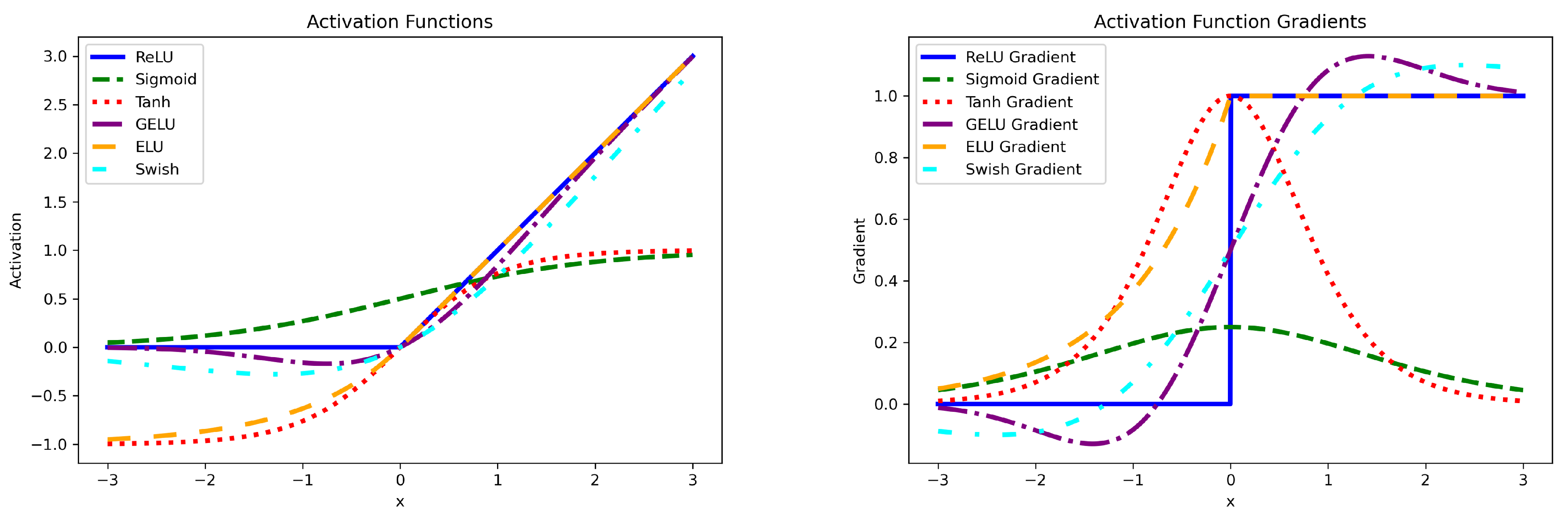