Abstract
This paper is about deriving the necessary and sufficient conditions of a surface family pair with a Bertrand pair as common geodesic curves in Galilean 3-space . Thereafter, the consequence for the ruled surface family pair is also deduced. Meanwhile, some examples are provided to show the surfaces family with common Bertrand geodesic curves.
MSC:
53A04; 53A05; 53A17
1. Introduction
Traditional study on curves and surfaces focus on how to realize specific curves, such as asymptotic curve, geodesic curve, principal curve, etc., on a display surface. However, the reciprocal problem, that is, acquired surfaces having a distinct curve, is considerably more motivating. The design of surfaces with a given distinct curve is a new study subject that entices the attention of many scholars. The first work in this subject of design was presented by Wang et al. [1]. They created a surface family over a common geodesic. Stimulated by Wang et al. [1], researchers established restrictions for a prescribed curve to be a distinct curve on designed surfaces [2,3,4,5,6,7,8,9,10,11,12].
In the theory of distinct curves, the congruous correlation through the curves is a good problem. One of the traditional distinct curves is the Bertrand curve. If the principal normal vectors of two curves are linearly correlated at their matching points, the two curves are said to be a Bertrand pair [13,14,15,16,17,18]. In the (three-dimensional) Galilean space , extra properties and descriptions of the Bertrand pair have been elaborated in a number of works; for example Abdel-Aziz and Khalifa considered a location vector of a random curve [19]. In addition, they imposed several conditions on the random curve’s curvatures in order to investigate specific curves and their Smarandache curves. The parametrization of a set of surfaces over a specific geodesic curve has been investigated by Yuzbas and Bektas. On the parametric surfaces, they constructed the necessary and sufficient conditions for this curve to be an iso-geodesic curve [20]. The problem of designing a hypersurface family with common geodesic curve in 4D Galilean space has been addressed in [21,22,23].
However, to our knowledge, no further work has been done to create surface family pairs with curve pairs that are geodesic curves. In order to cover this need, we investigate Bertrand pairs as geodesic curves and construct a surface family pair with a Bertrand pair as common geodesic curves. Furthermore, the extension to the ruled surfaces family is also described. Meanwhile, some examples are shown to construct the surfaces family and ruled surfaces family with common Bertrand geodesic curves.
2. Basic Concepts
The Galilean 3-space is a Cayley–Klein geometry provided with the projective metric of signature [16,17]. The absolute figure of the Galilean space depends on the organized triple {, L, I}, where is the (absolute) plane in the real 3-dimensional projective space (), L is the line (absolute line) in , and L is the stationary elliptic involution of points of L. Homogeneous coordinates in are endowed in such a manner that the absolute plane is given by , the absolute line L by , and the elliptic involution is given by . A plane is named Euclidean if it includes L, otherwise it is named isotropic; that is, planes x = const are Euclidean, and so is the plane . Other planes are isotropic. In other words, an isotropic plane has no isotropic orientation.
For any , and , their scalar product is
and their vector product is
where , , and are the standard basis vectors in .
A curve is named allowable curve if it has no inflection points, that is, and no isotropic tangents . An allowable curve is similar to a smooth curve in Euclidean space. For an allowable curve : represented by the Galilean invariant arc-length s, we have:
The curvature and torsion of the curve are
Note that an allowable curve has . The Serret–Frenet vectors are:
where , , and , respectively, are the tangent, principal normal, and binormal vectors. For every point of , the Serret–Frenet formulae read:
The planes that match the subspaces Sp{ }, Sp{, }, and Sp{, }, respectively, are named the osculating plane, normal plane, and rectifying plane.
Definition 1
([13,14,15,24]). Let and be two allowable curves in ; and are principal normal vectors of them, respectively; the pair {, } is named a Bertrand pair if and are linearly dependent at the corresponding points; is named the Bertrand mate of ; and
where f is a constant.
We indicate a surface M in by
If , the isotropic surface normal is
which is orthogonal to each of the vectors and .
Definition 2
([1,2,3,4,5,6,7,8,9,10,11,12,13,14,15,16,17,18,19,20,21,22,23,24]). A curve on a surface is geodesic if and only if the surface normal is everywhere parallel to the principal normal vector of the curve.
An isoparametric curve is a curve on a surface that has a constant s or t-parameter value. In other terms, there exists a parameter such that or . Given a parametric curve , we call it an isogeodesic of the surface if it is both a geodesic and a parameter curve on .
3. Main Results
This section presents a new approach for constructing a surface family pair interpolating a Bertrand pair as mutual geodesic curves in . To do this, we take into account a Bertrand pair such that the surface’s tangent planes are coincident with the curve’s rectifying planes.
Let be an allowable curve, is Bertrand mate of , and , is the Frenet–Serret frame of as in Equation (6). The surface family M interpolating can be written as [18]
Similarly, the surface is specified by
Here, and are named directed marching-scale functions.
In order to show that is a geodesic curve on M, according to Equation (10), we discuss what the marching-scale functions should satisfy. Therefore, we have
and
Since is iso-parametric on M, there exists a value such that ; that is,
Hence, when —i.e., over , we have
The coincidence of the principal normal with the surface normal recognizes as a geodesic curve. We let {, M} denote the surface family pair. Hence, we have the following theorem:
Theorem 1.
{, M} interpolate {, } as common geodesic curves if and only if the following conditions
are satisfied.
For the above conditions in Theorem 1, and can be written as:
Here, , , and are nowhere vanishing functions. Hence, from Theorem 1, we gain:
Corollary 1.
If and as in Equations (17), the sufficient and necessary condition is
For suitability in performance, and can be chosen in two special forms:
- (1)
- Ifthen,where and are functions, and , and are nowhere vanishing functions.
- (2)
Example 1.
According to Corollary 1, we have:
- (1)
- If , , , then Equation (18) is satisfied. Then, the set {, M} interpolates {, } as common geodesic curves as in (Figure 1):where the blue curve represents , the green curve is , , and .
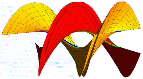 Figure 1. M (yellow) and (red).
 - (2)
- If , , , then Equation (16) is satisfied. Then, the set {, M} interpolates {, } as common geodesic curves as in (Figure 2):andwhere the blue curve represents and the green curve is where s, .
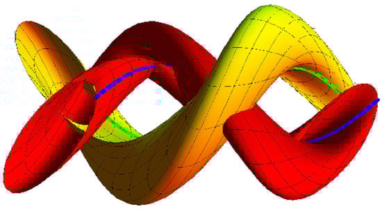 Figure 2. M (yellow) and (red).
Ruled Surfaces Family with Common Bertrand Geodesic Curves
Ruled surfaces are simple and common surfaces in geometric designs. Suppose is a ruled surface with the directrix , and is also an isoparametric curve of , then there exists such that . Consequently, the surface can be represented as
where (, and defines the direction of the rulings. In view of Equation (10), we have
which is a system of equations in two unknown functions and . For and , we have
The necessary and sufficient conditions for to be a ruled surface with a directrix ; are represented in Equation (24).
In Galilean 3-space , it is demonstrated there exist only three types of ruled surfaces realized as follows [17]:
- Type I.
- Non-conoidal or conoidal ruled surfaces with striction curve do not lie in a Euclidean plane.
- Type II.
- Ruled surfaces with striction curve in a Euclidean plane.
- Type III.
- Conoidal ruled surfaces with absolute line as the oriented line in infinity.
We now check if the curve is also geodesic on these three types:
- Type I.
- Type II.
- Type III.
Equation (30) satisfies Theorem 1. Thus, at all points on , the ruling , . Further, the ruling and the vector should not be parallel. Thus,
for functions , and . Replacing it into Equation (24), we get
Hence, the ruled surface family with the common geodesic base curve can be written as
where and can control the form of the surface family. It is clear that
Thus, when , that is, along , the surface normal is
Theorem 2.
The sufficient and necessary condition for being a ruled surface with as a geodesic is that there exists a parameter , as well as the functions and , so that can be specified by
where .
It must pointed out that, in this family, there exist two geodesic curves crossing through each point on : one is itself and the other is a non-isotropic line in the orientation as in Equation (32). All components of the isogeodesic ruled surfaces are specified by the two functions and , that is, by the orientation non-isotropic vector function . Similarity, the ruled surfaces of type III has also have as an isogeodesic curve.
Corollary 3.
The only ruled surfaces {, } of type III interpolate the Bertrand pair as common geodesic curves.
Now, we research the correlations of the ruled surface family of type III. Let , be a curve with , from Equations (7), (29) and (30); we have . From Equations (10), (11) and (31), the ruled surfaces family of type III that interpolate the Bertrand pair as common geodesic curves is
where f is a constant, satisfies Equation (31), , and .
Example 2.
In view of Example 1, we have:
- (1)
- If , , the ruled surfaces family {, } interpolates {, } as common geodesic curves as in (Figure 3):where the blue curve represents , the green curve is , , and .
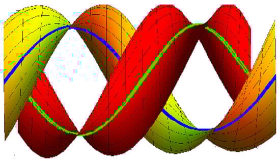 Figure 3. M (yellow) and (red).
 - (2)
- If , , the ruled surfaces family {, } interpolates {, } as common geodesic curves as in (Figure 4):where the blue curve represents , the green curve is , , and .
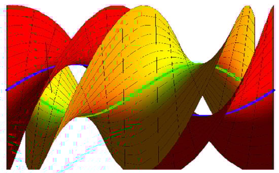 Figure 4. M (yellow) and (red).
 - (3)
- If , , the ruled surfaces family {, } interpolates {, } as common geodesic curves as in (Figure 5):where the blue curve represents , the green curve is , , and .
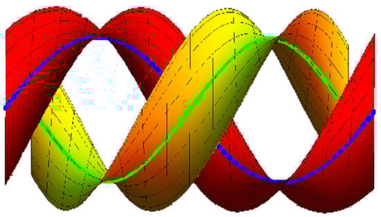 Figure 5. M (yellow) and (red).
4. Conclusions
In this work, we constructed the surfaces family and ruled surfaces family having Bertrand curves as common geodesic curves in Galilean space . For any allowable curve, there only exists the ruled surfaces family of type III having the same curve as common geodesic curves. Meanwhile, some curves were selected to organize the surfaces family and ruled surfaces family that have common Bertrand geodesic curves.
Hopefully, these results will be advantageous to physicists and those exploring general relativity theory. There are numerous opportunities for additional work; for example, consider the pseudo-Galilean geometry as a counterpart to the problem presented in the current study.
Author Contributions
Conceptualization, A.A.A. and R.A.A.-B.; methodology, R.A.A.-B.; validation, A.A.A. and R.A.A.-B.;formal analysis, A.A.A. and R.A.A.-B.; investigation, R.A.A.-B.; resources, A.A.A. and R.A.A.-B.; data curation, A.A.A. and R.A.A.-B.; writing—original draft preparation, R.A.A.-B.; writing—review and editing, A.A.A.; visualization, R.A.A.-B.; supervision, R.A.A.-B.; project administration, A.A.A.; funding acquisition, A.A.A. All authors have read and agreed to the published version of the manuscript.
Funding
This research was funded by Princess Nourah bint Abdulrahman University Researchers Supporting Project number (PNURSP2023R337).
Data Availability Statement
Not applicable.
Acknowledgments
The authors would like to acknowledge the Princess Nourah bint Abdulrahman University Researchers Supporting Project number (PNURSP2023R337), Princess Nourah bint Abdulrahman University, Riyadh, Saudi Arabia.
Conflicts of Interest
The authors declare no conflict of interest.
References
- Wang, G.J.; Tang, K.; Tai, C.L. Parametric representation of a surface pencil with a common spatial geodesic. Comput. Aided Des. 2004, 36, 447–459. [Google Scholar] [CrossRef]
- Kasap, E.; Akyldz, F.T.; Orbay, K. A generalization of surfaces family with common spatial geodesic. Appl. Math. Comput. 2008, 201, 781–789. [Google Scholar] [CrossRef]
- Li, C.Y.; Wang, R.H.; Zhu, C.G. Parametric representation of a surface pencil with a common line of curvature. Comput. Aided Des. 2011, 43, 1110–1117. [Google Scholar] [CrossRef]
- Li, C.Y.; Wang, R.H.; Zhu, C.G. An approach for designing a developable surface through a given line of curvature. Comput. Aided Des. 2013, 45, 621–627. [Google Scholar] [CrossRef]
- Bayram, E.; Guler, F.; Kasap, E. Parametric representation of a surface pencil with a common asymptotic curve. Comput. Aided Des. 2012, 44, 637–643. [Google Scholar] [CrossRef]
- Liu, Y.; Wang, G.J. Designing developable surface pencil through given curve as its common asymptotic curve. J. Zhejiang Univ. 2013, 47, 1246–1252. [Google Scholar]
- Atalay, G.S.; Kasap, E. Surfaces family with common Smarandache geodesic curve. J. Sci. Arts 2017, 4, 651–664. [Google Scholar]
- Atalay, G.S.; Kasap, E. Surfaces family with common Smarandache geodesic curve according to Bishop frame in Euclidean space. Math. Sci. Appl. 2016, 4, 164–174. [Google Scholar] [CrossRef]
- Bayram, E.; Bilici, M. Surface family with a common involute asymptotic curve. Int. J. Geom. Methods Mod. Phys. 2016, 13, 447–459. [Google Scholar] [CrossRef]
- Guler, F.; Bayram, E.; Kasap, E. Offset surface pencil with a common asymptotic curve. Int. J. Geom. Methods Mod. Phys. 2018, 15, 1850195. [Google Scholar] [CrossRef]
- Atalay, G.S. Surfaces family with a common Mannheim asymptotic curve. J. Appl. Math. Comput. 2018, 2, 143–154. [Google Scholar]
- Atalay, G.S. Surfaces family with a common Mannheim geodesic curve. J. Appl. Math. Comput. 2018, 2, 155–165. [Google Scholar]
- Elzawy, M.; Mosa, S. Quaternionic Bertrand curves in the Galilean space. Filomat 2020, 34, 59–66. [Google Scholar] [CrossRef]
- Abdel-Aziz, H.S.; Saad, M.K. Darboux frames of Bertrand curves in the Galilean and Pseudo-Galilean spaces. JP J. Geom. Topol. 2014, 16, 17–43. [Google Scholar]
- Jiang, X.; Jiang, P.; Meng, J.; Wang, K. Surface pencil pair interpolating Bertrand pair as common asymptotic curves in Galilean space 𝔾3. Int. J. Geom. Methods Mod. Phys. 2021, 18, 2150114. [Google Scholar] [CrossRef]
- Roschel, O. Die Geometrie des Galileischen Raumes; Habilitationsschrift, Montanuniversität Leoben: Leoben, Austria, 1984. [Google Scholar]
- Divjak, B. Geometrija Pseudogalilejevih Prostora. Ph.D. Thesis, University of Zagreb, Zagreb, Croatia, 1997. [Google Scholar]
- Abdel-Baky, R.A.; Alluhaib, N. Surfaces family with a common geodesic curve in Euclidean 3-Space 𝔼3. Int. J. Math. Anal. 2019, 13, 433–447. [Google Scholar] [CrossRef]
- Abdel-Aziz, H.S.; Khalifa, M.S. Smarandache curves of somr special curves in the Galilean 3-space 𝔾3. Honam Math. J. 2015, 37, 253–264. [Google Scholar] [CrossRef]
- Yuzbası, Z.K.; Bektas, M. On the construction of a surface family with common geodesic in Galilean space 𝔾3. Open Phys. 2016, 14, 360–363. [Google Scholar] [CrossRef]
- Yoon, D.W.; Yuzbası, Z.K. An approach for hypersurface family with common geodesic curve in the 4D Galilean space 𝔾4. Pure Appl. Math. 2018, 25, 229–241. [Google Scholar]
- Altin, M.; Kazan, A.; Karadag, H.B. Hypersurface family with smarandache curves in Galilean 4-space. Commun. Fac. Sci. Univ. Ank. Ser. A1 Math. Stat. 2021, 7, 744–761. [Google Scholar] [CrossRef]
- Makki, R. Hypersurfaces with a common asymptotic curve in the 4D Galilean space 𝔾4. Asian-Eur. J. Math. 2022, 15, 2250199. [Google Scholar] [CrossRef]
- Öğrenmiş, A.O.; Öztekin, H.; Ergüt, M.E. Bertrand curves in Galilean space and their characterizations. Kragujev. J. Math. 2009, 32, 139–147. [Google Scholar]


Disclaimer/Publisher’s Note: The statements, opinions and data contained in all publications are solely those of the individual author(s) and contributor(s) and not of MDPI and/or the editor(s). MDPI and/or the editor(s) disclaim responsibility for any injury to people or property resulting from any ideas, methods, instructions or products referred to in the content. |
© 2023 by the authors. Licensee MDPI, Basel, Switzerland. This article is an open access article distributed under the terms and conditions of the Creative Commons Attribution (CC BY) license (https://creativecommons.org/licenses/by/4.0/).