Abstract
Any small environmental changes in the driving environment of a traffic vehicle can become a risk factor directly leading to major safety incidents. Therefore, it is necessary to assist drivers in automatically detecting risk factors during the driving process using algorithms. However, besides making it more difficult for drivers to judge environmental changes, the performance of automatic detection networks in low illumination scenarios can also be greatly affected and cannot be used directly. In this paper, we propose a risk factor detection model based on deep learning in low illumination scenarios and test the optimization of low illumination image enhancement problems. The overall structure of this model includes dual discriminators, encoder–decoders, etc. The model consists of two main stages. In the first stage, the input low illumination scene image is adaptively converted into a standard illumination image through a lighting conversion module. In the second stage, the converted standard illumination image is automatically assessed for risk factors. The experiments show that the detection network can overcome the impact of low lighting and has high detection accuracy.
Keywords:
neural network; risk factor detection; low illumination images; artificial intelligence; deep learning MSC:
68T45
1. Introduction
Risk factors encountered by vehicles used for transportation in the driving environment can directly lead to major safety incidents, posing significant risks to traffic safety. Therefore, it is necessary to use algorithms to assist drivers in automatically detecting risk factors during driving.
Prior to this study, work related to high dynamic range (HDR) involved low illumination image processing, which needs to collect the same scene under various lighting conditions and then align and merge the results into a highly reproducible image output. This method has a certain reference value, but it cannot handle a single low illumination input, which is different from the application scenario in this method. Among the traditional techniques used for low illumination image detection and processing, the most representative methods are the adaptive histogram equalization (AHE), optical neural network, and multi-scale optical neural network model [1].
With the rapid development of deep learning in the field of computer vision, object detection based on deep learning has shown good performance in standard scenes [2,3,4], such as scenes with good lighting conditions, and can meet the requirements of assisting drivers in the automatic detection of risk factors while driving in standard scenes [5,6]. However, this method is not suitable for special scenes. For example, in low illumination scenarios, the accuracy of object detection will be greatly reduced. The main reason for this limitation is that most of the simulation scenes used in algorithm design are standard scenes [7,8,9,10], which makes them unable to adapt to changes and interference caused by low illumination scenes in target texture, structure, and color characteristics [11,12]. However, in real life, the probability of low illumination scenes appearing is relatively high (such as night scenes), and low illumination scenes can have a more serious impact on the driver’s judgment. Therefore, it is of great significance to propose an automatic detection algorithm for low illumination object detection. Section 2 of this article introduces and discusses the current mainstream research content of the two basic tasks of conversion and detection. Section 3 introduces the process and specific content of our method. Section 4 presents our experimental results and analyses them. Section 5 summarizes the entire article and outlines our next plans.
To solve the above problems, we propose a risk factor detection model based on deep learning in low illumination scenarios and test the optimization of low illumination image enhancement. The overall structure includes a dual discriminator, encoder–decoder, etc. The model consists of two main stages [13,14]. In the first stage, the input low illumination scene image is adaptively converted into a standard illumination image through a lighting conversion module. In the second stage, the converted standard illumination image is automatically detected for risk factors. Experiments have shown that risk factors can be detected in low illumination scenarios with high detection accuracy. Our main contributions are summarized as follows:
- (1)
- We propose an adaptive enhanced detection network structure for low illumination object detection, which effectively integrates dual discriminators, encoding decoders, and attention mechanisms.
- (2)
- We designed the lighting conversion stage as the first stage of the global model, which can be applied to the standardized training of pairwise image data to achieve adaptive enhancement of low illumination image data, thus preventing input images with spatially varying lighting conditions from experiencing overexposure or underexposure problems after enhancement.
- (3)
- We designed the risk factor detection phase as the second phase of the global model. This part of the model is mainly based on the Transformer algorithm, adopts an encoder–decoder structure, and is subjected to lightweight processing, which can effectively process the adaptive enhanced image output in the first stage. On this basis, optimization is carried out for small target detection and the entire detection process to improve the overall automatic detection performance of risk factors.
- (4)
- We demonstrated the adaptive conversion effect of the first stage model on images of whole or partial regions through comparative experiments and demonstrated through ablation experiments that the detection performance of the second stage can be improved after adaptive conversion in the first stage. Based on quantitative experiments, it was shown that the second-stage detection model is generally superior to the mainstream CNN (convolutional neural network) and that the first stage can overcome the impact of low illumination in whole or partial region on detection. The global network can be used for low illumination object detection and has good detection performance.
2. Related Works
In terms of deep learning, there is generally less demand for low illumination scene object detection in the industry, so there is little work discussing or implementing the two tasks of illumination conversion and object detection through a single method. At the same time, in terms of illumination conversion, existing deep learning methods have high requirements for the dataset, and most of them need to process normal illumination images to form a one-to-one correspondence between low illumination images and normal illumination images [15,16]. For example, the authors in [17] proposed an end-to-end framework that applies Retinex theory to deep networks. In HDR, deep learning methods have also emerged for multi-frame low-light enhancement [18,19]. In terms of detection, due to the good detection performance of Transformer [20] in the field of computer vision, the research focus of detection models has gradually shifted from CNN-class models to Transformer-class models. However, in the process of designing relevant models, all models are currently focused on conventional illuminance, and mainstream methods are unable to overcome the impact of illuminance, resulting in generally poor detection results in low illumination scenarios.
This section starts with the generation of adversarial networks and transformers corresponding to transformation and detection tasks in order to introduce the relevant research content adopted by current mainstream solutions.
2.1. Generate Adversarial Networks
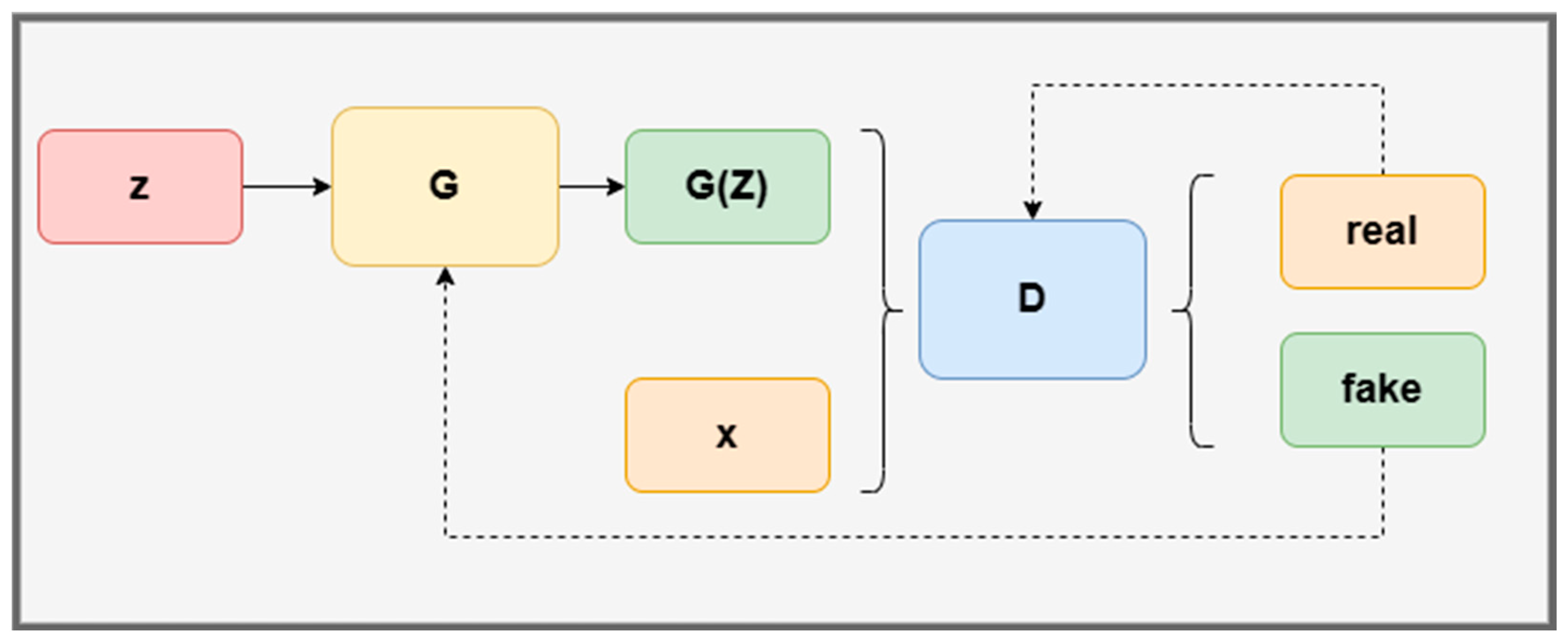
A basic generative adversarial network consists of a generator (G) and a discriminator (D), which achieve dynamic equilibrium through game confrontation. From a macro perspective, the generator (G) is used to generate images with the aim of bringing the generated images closer to real images [21,22,23]. The discriminator (D) is used to distinguish whether its input is a generated fake image or a real image, with the aim of distinguishing between the generated image and the real image. These images grow together in confrontation and eventually reach a Nash equilibrium state, making the generated results roughly equivalent to the real image.
Figure 1 shows the basic structure of a standard generated adversarial network. Here, G is represented as a parameterized neural network. The input is the noise variable z, which generates a sample G(z) that follows a specific distribution through G. If we assume that the real data follow a distribution, the real samples sampled from the data and G(z) are input into D, which determines whether the input samples come from the real data. The goal of D is to classify input samples reasonably. That is, the sample G(z) generated by G is classified as the fake class, and the real data sample is classified as the real class. On the other hand, G’s goal is to generate samples that can deceive D and be classified as real by D. Thus, there is an adversarial relationship between the two; this is the core idea behind generating adversarial networks. The main idea in the training process is to fix one network and train the other. After several iterations, Nash equilibrium was achieved.

Figure 1.
The basic structure of standard generative adversarial networks.
From a mathematical point of view, the goal of a network is to make the two distributions close together for the distribution of real data and the generation distribution with parameterization to concretize the abstract problem of generating data equal to real data. First, one can take n samples from the generated distribution and then use the maximum likelihood function to evaluate the parameters.
When fixing the generating network to make the discriminant network complete the training goal, the specific operation is to bring the likelihood function into the likelihood function when the likelihood function is maximum. This network can be regarded as a fixed discriminant network used to train the generating network. Then, we can obtain the Jensen–Shannon divergence (JSD) between the real distribution and generated distribution after resolving the total objective function. The above process can concretize the goal, transforming it from an abstract problem of narrowing the gap between the real distribution and generated distribution into a specific problem of narrowing the JSD between the two distributions. Therefore, the objective function for generating adversarial networks can be expressed as follows:
2.2. Transformer
Transformer is a deep learning neural network [20] that is primarily used in natural language processing but also has significant potential for computer vision applications. Transformer defect detection offers good global characteristics and uses a self-attention mechanism to extract intrinsic features of defects, allowing it to effectively obtain global information and map it to multiple spaces through multiple heads, with strong model expression ability.
Transformer splits the input image into multiple sequences of element blocks in which each element block can be meaningfully associated with other element blocks, thus achieving a better understanding of the overall image. This neural network uses multiple levels of attention mechanisms to allow each element block in the input sequence to have meaningful associations with other element blocks. Transformer is different from the previous SOTA model in that it allows all tasks to be analyzed at the same time using parallel task processing instead of serial processing. Meanwhile, common image description models based on the encoder–decoder system use CNN to extract deep features to encode hidden semantics contained in the image and then use RNN to decode semantics from the encoded deep features and generate image descriptions. However, Transformer has separate encoder and decoder structures. The encoder is mainly used to read element blocks in the input sequence and then establish connections with other element blocks through attention mechanisms. The decoder is used to generate output sequences and can use attention mechanisms to use the encoder’s output to generate better results.
3. Methods
3.1. Overall Framework Description
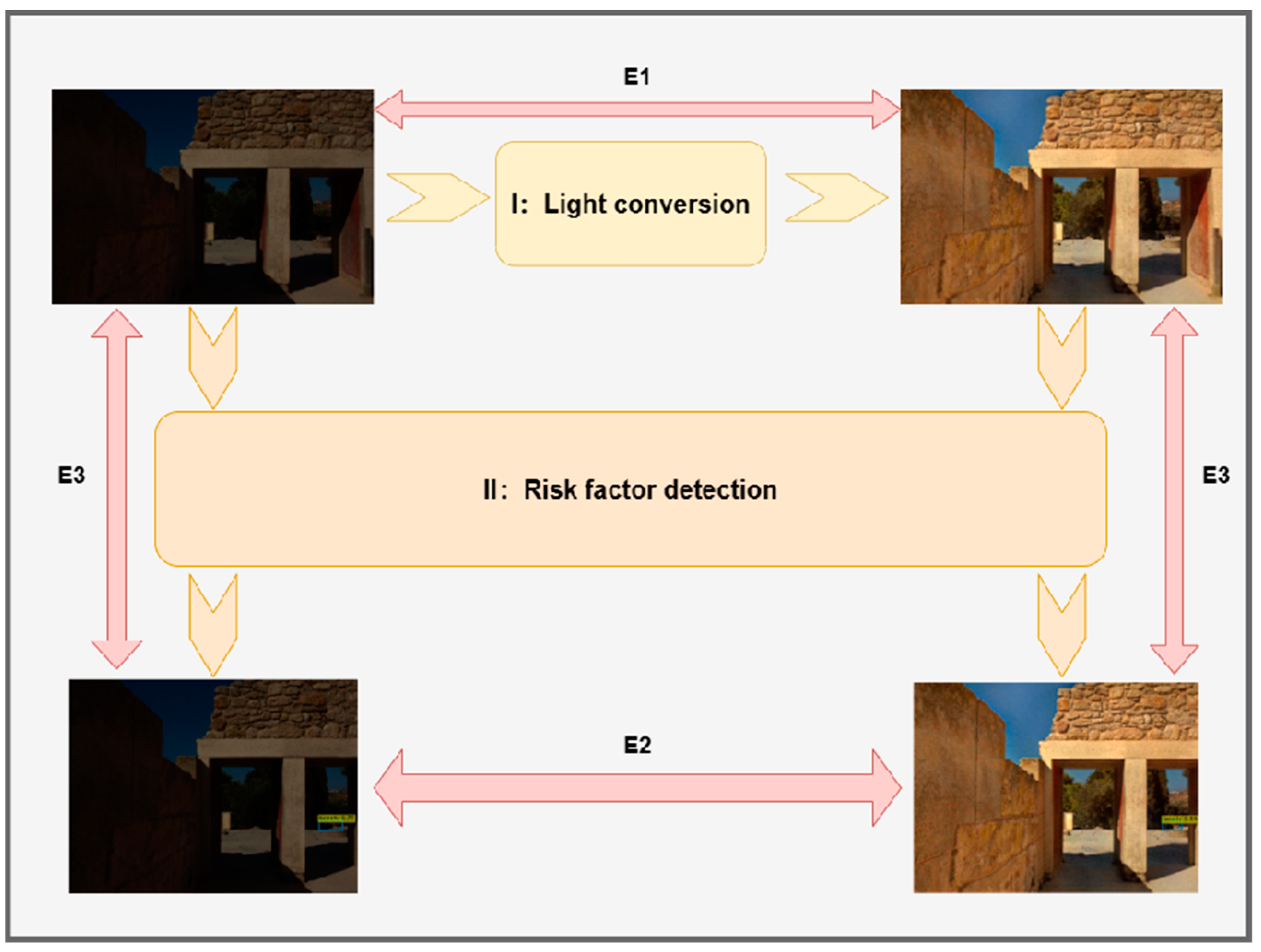
The goal of risk factor detection in low illumination scenes based on deep learning is to find potentially dangerous objects in the image and predict their category labels and bounding boxes. This process is essentially a set prediction problem, as the predicted objects do not require sorting. Before making predictions, it is necessary to overcome the impact of low illumination on detection accuracy. Thus, the whole structure of the model consists of two stages: light conversion and risk factor detection.
The purpose of the lighting conversion phase (I) design is to adaptively complete the conversion process from low lighting conditions to standard lighting. This module is based on the generation-game idea of generative adversarial networks and performs adaptive lighting restoration and enhancement on image data that are not properly paired [24,25,26], thus completing the transformation of lighting scenes. The purpose of the risk factor detection phase (II) design is to automatically detect risk factors in converted standard illumination images. This module is based on Transformer-class detection algorithms, adopts an encoder–decoder structure, and performs lightweight processing on the model according to requirements, thereby ensuring a certain degree of accuracy while accelerating detection speed and improving the overall automatic detection performance of the risk factors. Through the above steps, our method can overcome the interference caused by low illumination on detection and fill the application gap of the detection model in low illumination scenarios. This method is highly inclusive for input data and does not require paired low illumination samples. Simultaneously, this technique is suitable for low-light regional data and can intelligently improve selective areas without the problem of excessive exposure, commonly seen in traditional methods, leading to increased usability.
Figure 2 shows the overall workflow framework of the designed method, with three types of validation experiments (E1, E2, and E3), each of which incurs corresponding losses. Among them, E1 is used to compare the effects of the first-stage conversion, which generates loss of light conversion. E3 is used to demonstrate the effectiveness of using the second stage for detection, which results in loss detection. E2 is used to compare the effectiveness of second-stage detection after first-stage conversion, resulting in ablation detection loss. Experimental results and analysis are detailed in the experimental section.

Figure 2.
Method workflow framework.
3.2. Light Conversion
The lighting conversion part, which is in the first stage of the entire process, can train image data that are not standardized in pairs [27,28] without requiring low and normal illumination image data to correspond to each other in order to achieve adaptive enhancement of low illumination image data. This prevents input images with spatially varying lighting conditions from experiencing regional overexposure or underexposure after enhancement.
The core of this section is based on the adversarial game theory of generating adversarial networks [29,30,31]. Using a basic discriminator generator structure, the model can adapt to enhancement based on the illumination level of each region of the input image and use self-feature loss to constrain the perceptual similarity of the transformation process, thereby ensuring that the image content features do not change before and after enhancement [32]. At this stage, a series of optimizations was created for multi-scale image synthesis and adaptive enhancement based on the basic core algorithms, including a U-net structure generator with an attention mechanism, a dual discriminator, and the loss of both generation and self-functioning.
3.2.1. Generation Phase
The basic structure of the first phase consists of two parts: generation and discrimination. The two constrain each other through adversarial thinking, thereby learning and shortening the geometric distribution distance of the same features of the image under low and normal lighting and achieving dynamic balance during the training process.
In the generation process, the generator structure is designed using a U-net structure with an attention mechanism that can extract image features from multiple scales through multiple iterations of downsampling. This structure preserves a large amount of texture information in the image and can synthesize images containing multi-scale information, resulting in higher-quality generated images. At the same time, in order to adaptively enhance the illumination of low illumination images, we focus on enhancing the illumination of dark areas in the image, randomly sample small domain blocks from multiple scales, and put the images into the discrimination stage for discrimination. To ensure the consistency of features across scales, a self-regulatory attention mechanism is added as a constraint. This mechanism adjusts the attention map size to fit the feature map and multiplies it with all intermediate feature maps and output images to regularize the image itself. The self-normalization attention map is used to extract the light distribution of the input three-channel image as L and then perform normalization processing to (0, 1). Then, we calculate the element difference 1-L of the light distribution of the normalized image, which is used as the self-normalization attention map.
The overall structure of the designed generator is shown in Figure 3. It is mainly composed of down convolution blocks and up convolution blocks, which are used to extract multi-scale features from the image feature layer. The two modules contain a total of eight convolutional blocks, with each block mainly composed of two joint convolutional layers. Each joint convolutional layer includes 3 × 3 convolutional layers, activation layers, and batch normalization layers. In the downsampling stage, a maximum pooling layer is added; in the upsampling stage, a bilinear upsampling layer is used to replace the standard deconvolution layer to improve the generation effect.
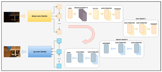
Figure 3.
Generator Network Structure.
3.2.2. Discrimination Phase
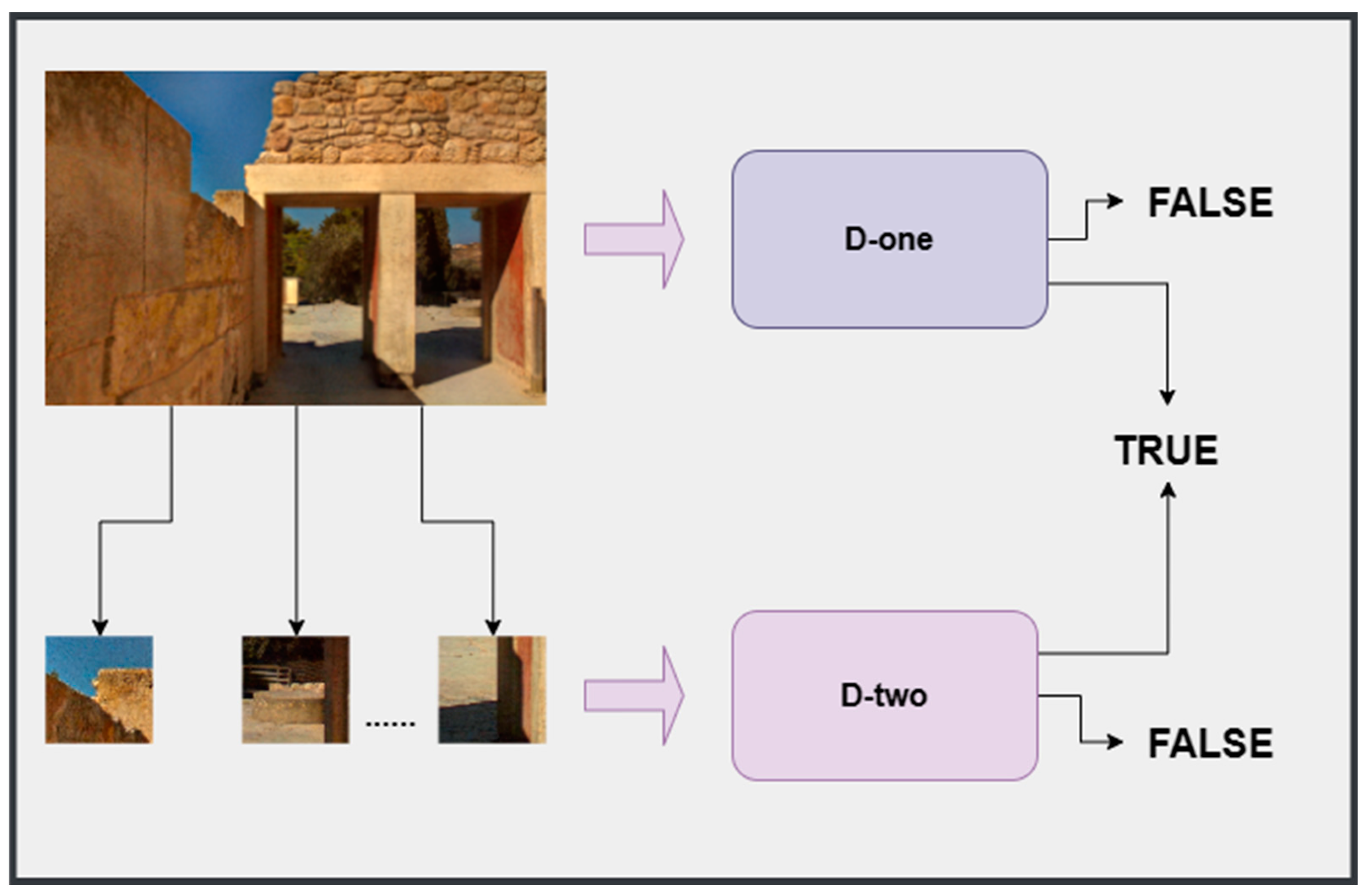
In the discriminator section, adversarial loss is used to represent and minimize the distance between the true illumination distribution and normal illumination distribution. However, in conventional models, when using a single discriminator to distinguish images, the center of gravity of discrimination covers the entire image, which cannot realize the adaptive enhancement of lighting conditions with spatial changes. For example, in a small area with high illumination in a low illumination background, the training process cannot adaptively enhance the low illumination of the background while slightly improving the overall lighting conditions, i.e., enhancing the overall image illumination while preventing local overexposure. Therefore, in the overall architecture design, the work of expanding the discrimination stage not only discriminates against the overall image but also randomly diverts attention to the details in the image to judge the enhancement effects of the details.
Therefore, in this study, a double-discriminator structure is designed and used according to the appropriate requirements. In addition to the regular discriminator, random clipping is performed from the output and true normal illumination images, and training is used to learn whether local image blocks are true normal illumination images or generated enhanced illumination images. This process acts as a workflow for a new discriminator. The basic structure of each discriminator consists of convolution, a fully connected layer, and dense connected layer. The logical relationship between the two discriminators is shown in Figure 4. The dual discriminator composed of the new discriminator and the original discriminator can solve the problems of local overexposure and underexposure and then realize adaptive enhancement of lighting conditions with spatial variation in the image.

Figure 4.
Double-discriminator Network Structure.
3.2.3. Conversion Loss
The loss function of the first stage model algorithm is mainly composed of two parts: the generated loss and the self-preserving loss feature. With a two-part restriction, the network model can be guaranteed to develop in the desired direction during the training process.
Generation loss is generated by generators and discriminators over the course of counterplay. Generation loss is used to describe the geometric distance between the generated data distribution and the actual data distribution. The discriminator uses functions to estimate the probability that the real data are more true than the generated data in order to prompt the generators to generate false data that are more true than the real image and to discriminate the quality of the generated samples using a double discriminator structure. Discriminators typically measure the quality of the generated data by measuring the physical distance between the generated data and the real data. However, different references correspond to different results. When we measure real data by using the generated data as a reference, it can be expressed as:
Conversely, when we swap references and results, we can get formulas representing the same physical distance but with different expressions, as shown in Equation (3) below; this means we can further confirm the physical distance between the generated data and the actual data through comparison.
where PB is the discriminator structure and represents the sample separately from the true and biochemical distributions, and σ is an activation function, in which the sigmoid function is used. In our method, we use this principle to design a bidirectional loss limiting constraint, which can be expressed as:
Thus, the loss function of the first discriminator (D) and generator (G) in the double discriminator is expressed as
Similarly, for the composite structure in the double discriminator, we select some areas for separate comparison. After a lot of training, we can ensure that random slices can cover most areas in the input image, thus ensuring the constraint on the conversion effect of local low-light images:
Loss of self-feature preservation is used to constrain perceived similarity. A common practice is to model the spatial distance of features between images using a pre-trained convolutional neural network to limit the feature distance between the extracted output image and its ground truth.
To emphasize the effect of self-regulation, we ensure that image content features do not change as much as possible before and after enhancement. We translate this problem into a characteristic VGG distance between the input low light and its enhanced normal light output. In this way, the distance between the outputs is limited by the loss of self-characteristics, which is defined as
where is the initial input image and G() is the enhanced image generated by the generator; is the feature graph extracted from the pre-trained convolutional neural network model VGG; i represents the ith largest pooled layer and j represents the jth convolutional layer after the ith largest pooled layer; and and are the dimensions of the extracted signature graph.
For the second discriminator in the double discriminator, the input and output image clipping blocks are also constrained by self-characteristic loss, so the overall loss function for this part of the light conversion model can be written as
3.3. Risk Factor Detection
The second stage of the entire process involves the automatic risk factor detection of converted standard illumination images after the first stage of the process. This model is mainly based on the Transformer algorithm and adopts an encoder–decoder structure. The model is designed to be lightweight, according to the requirements of completing optimization of the entire detection process and improving the overall automatic detection performance of the risk factors.
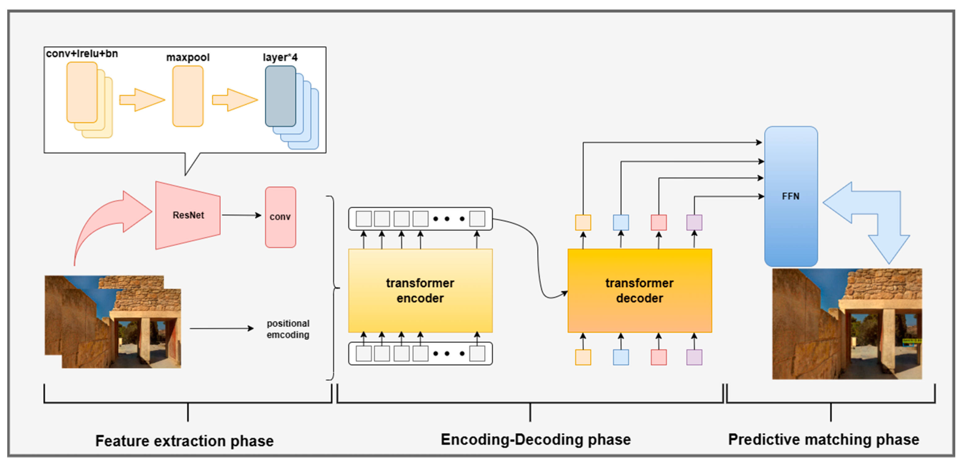
The overall model is an end-to-end framework with a basic structure consisting of three parts: feature extraction, encoding–decoding [33,34], and prediction matching. The detection model designed in this paper has a simpler pipeline than that used in mainstream convolutional neural network class detection, which eliminates NMS and the anchor [35,36,37,38]. Therefore, this model learns the position encoding and passes it on to the input, simultaneously using the bounding box predictor instead of MLP for further lightweight model processing. Through experiments, it was demonstrated that the detection task can be completed with high detection accuracy. The basic structure of the second stage risk factor detection model mainly consists of three stages: feature extraction, encoding–decoding, and prediction matching, as shown in Figure 5.

Figure 5.
Basic structure of the risk factor detection model.
3.3.1. Feature Extraction Phase
The model’s feature extraction process, also known as the backbone network, is used to extract high-latitude features of images. At the same time, the depth of the network will directly affect the efficiency of feature extraction. However, if the network depth is simply increased, the performance will quickly decline when the network reaches a certain depth saturation. Thus, at this stage, the design adopts a residual layer structure to prevent the problem of a gradient disappearance or explosion during the deep propagation of information through the network, where each layer of information decreases or increases. The residual layer structure adds a transfer branch, allowing the loss to propagate the model gradient across network layers through the branch, thus alleviating network weakening caused by the model depth.
In the feature extraction phase, the input is first propagated to the mean pooling layer via ResNet-50; then, the 2048-dimensional feature map is converted into a 256-dimensional feature map via the convolutional layer. Finally, position encoding is constructed by encoding the position information of the input image.
3.3.2. Encoding–Decoding Phase
The encoding–decoding step processes the extracted image feature map and the constructed position encoding of the preceding portion through the encoding decoder structure. In the encoding preprocessing stage, serialize the input feature map and position encoding, and then input them into the encoder–decoder to obtain Transformer-based detection results. After the backbone, the self-attention mechanism performs global analysis on the feature map because the last feature map performs significantly better at detecting targets than the entire map. Therefore, performing self-attention on top of the feature map will enable the network to better extract the relationships between different large objects at different positions. Transformer performs better at detecting large targets than convolutional network models. Simultaneously incorporating positional encoding reflects image information in both the x and y dimensions.
3.3.3. Predictive Matching Phase
The design of the prediction matching phase is mainly to solve the two problems of prediction classification and matching position based on the input of the previous phase. Therefore, the overall structure of this stage is designed into two branches: one for predicting the target category and the other for predicting the bounding box. The prediction category branch includes a connection layer and a hidden layer with a dimension of 512. The predicted bounding box branch includes three connection layers and a hidden layer with a dimension of 512. The output layer has a dimension of four, and a sigmoid layer is added to ensure a positive final count. In the coding–decoding and prediction processes, attention modules are introduced to optimize the detection process. The final FFN is then calculated using a three-layer convolutional layer with the ReLU activation function and hidden layers. We next standardize the center coordinates, height, and width of the FFN prediction box and activate the box using the SoftMax function to obtain the prediction class label.
3.3.4. Detection Loss
In the second stage, the training direction of the model constrained by the loss function has two branches [39]. The first part is the category loss generated by classification, which is a constraint of target classification predictions. The loss is calculated via cross entropy using the image classification network. The second part is regression loss, which describes the size and accuracy loss of target position box prediction and is used to constrain target position matching during the training process. This loss includes the absolute value error and the global intersection ratio error in calculating the center point coordinates and width height parameters of the bounding box. Due to the need for a reference when calculating the position, there is a prerequisite for calculating this loss. The classification of the target must be the ground truth, that is, the loss of the target box is based on accurate classification of the target.
The initial setting of the maximum number of detections for a single sample is Localn = 100. In general, this maximum number of detections can be applied to actual usage needs. During the decoding process, a prediction set p = Localn containing results is generated based on the truth target set r. If the number of truth targets is less than the maximum Localn detection number, the missing element number is filled with a non-target identifier. Each truth element in the set includes the target class label and the truth box position parameter. Afterwards, through training, a ranking was found to minimize the distance between the two sets. This set can be expressed as the following equation, wherein the matched consumption of is between the true value and the predicted value. This method is more efficient than mainstream anchor box or prompt box matching methods. Direct one-on-one matching between sets effectively eliminates the loss caused by repeated matching:
In the second stage, the loss function must calculate all matching pairs, which is mainly a linear combination of the negative log likelihood of category predictions and prediction box losses of the guess target’s location. This function can be expressed as the following equation, where is the optimal matching order, is the target class label, and when the truth element is an objectless filling element, . Here, is a vector that defines the box position parameters (box center coordinates, height, and width relative to image size), and represents the probability of defining the category label as :
4. Results
4.1. Data and Experimental Settings
The method proposed in this paper uses the Python deep learning toolkit. The training and validation process of the experiment was carried out using a local host in the laboratory with two Nvidia3090 GPUs, a Core i9 CPU, and 32 G memory modules.
In the first stage of the experiment, the model can be trained using unpaired low illumination and conventional illumination images. As the core of this method involves dealing with detection problems in low illumination scenes in addition to normal illumination images, low illumination images are also required during the training process, and the proportion of low illumination images should be large enough. Due to the unique nature of this requirement, public datasets cannot be used directly. In total, 897 low illumination images and 1025 conventional illumination images were selected from the public dataset. The requirements for images with different illuminance values are relatively broad and do not need to correspond to each other. In order to demonstrate the performance of the dual discriminator in this method, about 10% of low illumination images are regional low illumination images. To ensure the experimental results, the established dataset was subjected to data augmentation, followed by removing images between low and conventional illumination and converting all images to the PNG format, with a uniform resolution adjustment of 600 * 400 pixels. The test process is used to select natural environmental images that were not used in the training (overall low illumination or partial low illumination). The first stage of training went through 100 iterations, with a learning rate of 1 × 10⁻⁴. Then, after another 100 iterations, the learning rate linearly decayed to 0. During this process, we used the Adam optimizer and set the batch size to 32.
The second stage of the model training process in this experiment used the publicly available COCO dataset, which contains a total of 118 k real-type images for training, all with annotations for truth detection boxes. Each image has a maximum of 63 detection instances, with an average of seven detection instances. The test process used images converted in the first stage, and in the comparison experiment, images before and after conversion were used for comparison. In the second stage of the training experiment, the Adam optimizer was used to set the initial learning rate as 1 × 10⁻⁴, the learning rate of the backbone network as 1 × 10⁵, and the weight attenuation as 1 × 10⁻⁴. The backbone network used the ResNet model of imagenet pre-training.
The overall experimental design was divided into three parts (E1, E2, and E3). Experiments E1 and E2 demonstrated the performance of this method in processing low illumination images through visualization and comparison. The E3 experiment demonstrated the detection performance of this method for risk factors in low illumination scenes through quantitative results.
4.2. Conversion Effect Experiment (E1)
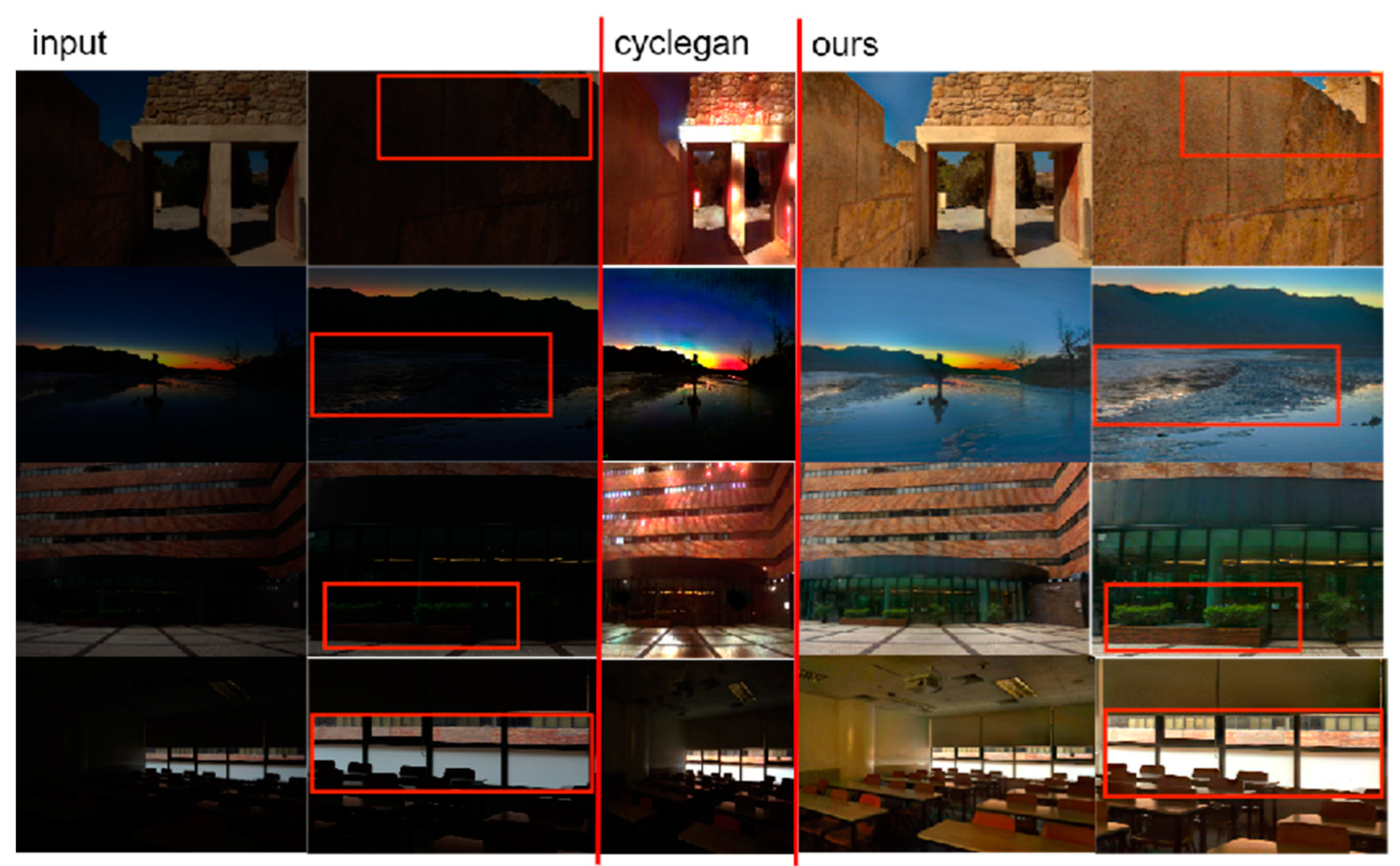
The conversion experiment results of the first stage model are shown in the figure below. The first column is the random input natural environment illumination image, the second column provides some details of the input image, the third column is the normal illumination image converted using the first stage model, and the fourth column presents some details of the normal illumination image.
The comparison of image details before and after the fourth line conversion shows that our method can adapt to low illumination images for conversion work (Figure 6). For areas with high illumination in the original image, the enhancement ratio will be reduced to prevent local illumination from being too bright and leading to distortion. A comparison of image details before and after conversion of the first three lines shows that the converted image can help people or machines obtain more detailed information about the original image hidden due to lighting problems.
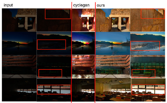
Figure 6.
Conversion experiment effects. (The annotated boxes in the figure highlight the significant contrasting regions of the experimental outcomes. Based on these areas, we can evaluate the conversion efficiency of the presented image).
At the same time, we conducted human subjective experiments commonly used in the field of conversion for our method and the mainstream conversion method CycleGAN. We randomly selected ten natural low illumination images and used CycleGAN and our method’s conversion stage for illumination conversion. We obtained 10 converted outputs, and then asked 10 subjects to independently compare these two outputs. Specifically, each person randomly received two out of 20 outputs and scored them. The scoring criteria reflected three aspects, with two points for each aspect and a maximum score of six points. The three aspects were as follows: (1) Is the image clear and does the image not contain any noise? (2) Are there no overexposed or underexposed areas in the image? (3) Are there no abnormal colors or distorted textures in the image? Figure 7 shows the scores of two output methods. Based on the results of the visual conversion experiments and human subjective experiments, we concluded that this method outperforms the current mainstream conversion methods in overcoming low illumination during the first stage.
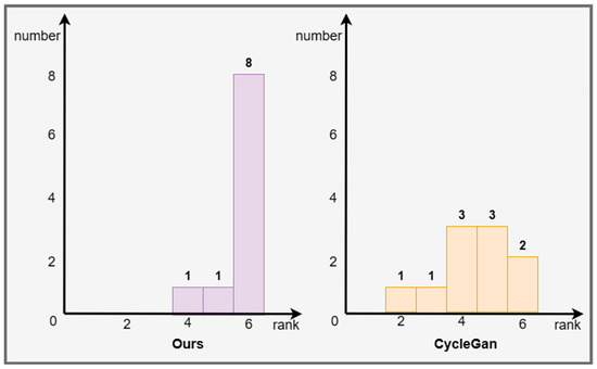
Figure 7.
Subjective human experimental results.
4.3. Ablation Detection Experiment (E2)
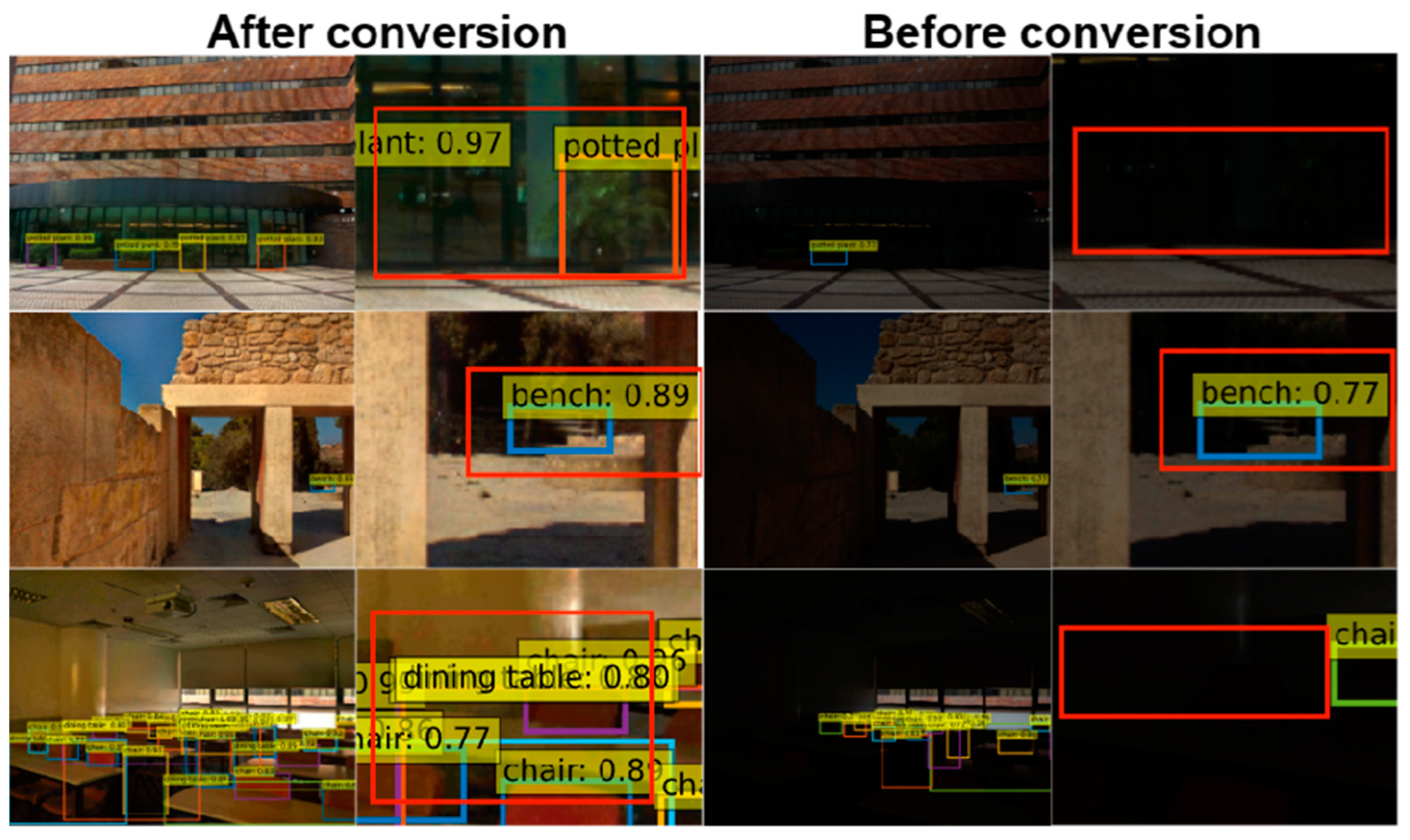
A comparison of detection and ablation experiment results using the first-stage conversion is shown in Figure 8. The first and second columns show the detection results and details after conversion, while the third and fourth columns show the pre conversion effects and details. The comparison between the first and third lines shows that after the first stage of adaptive transformation, this method can help detect objects that are not easily detected due to the influence of lighting in the second stage of the experiment. Based on the comparison of these three lines, it can be seen that after the first stage of adaptive transformation, the probability of confirming the detected object was improved, especially in the second line.

Figure 8.
Experimental results of ablation detection. (The highlighted annotation box in the figure indicates the area of significant contrast in the experimental findings. These fields enable us to assess the detection performance before and after the conversion.)
4.4. Risk Factor Confusion Quantification Experiment (E3)
This experiment used a fuzzy matrix to summarize the test records of the selected low illumination test set samples in the form of a matrix according to the true value and predicted value. The rows of the matrix represent true values, the columns of the matrix represent predicted values, the true values represent objectively existing risk factor targets in the sample, and the predicted values represent the risk factor targets predicted by the sample method. For each risk factor target, if it matched, it was recorded as True (0); if not, it was recorded as False (1).
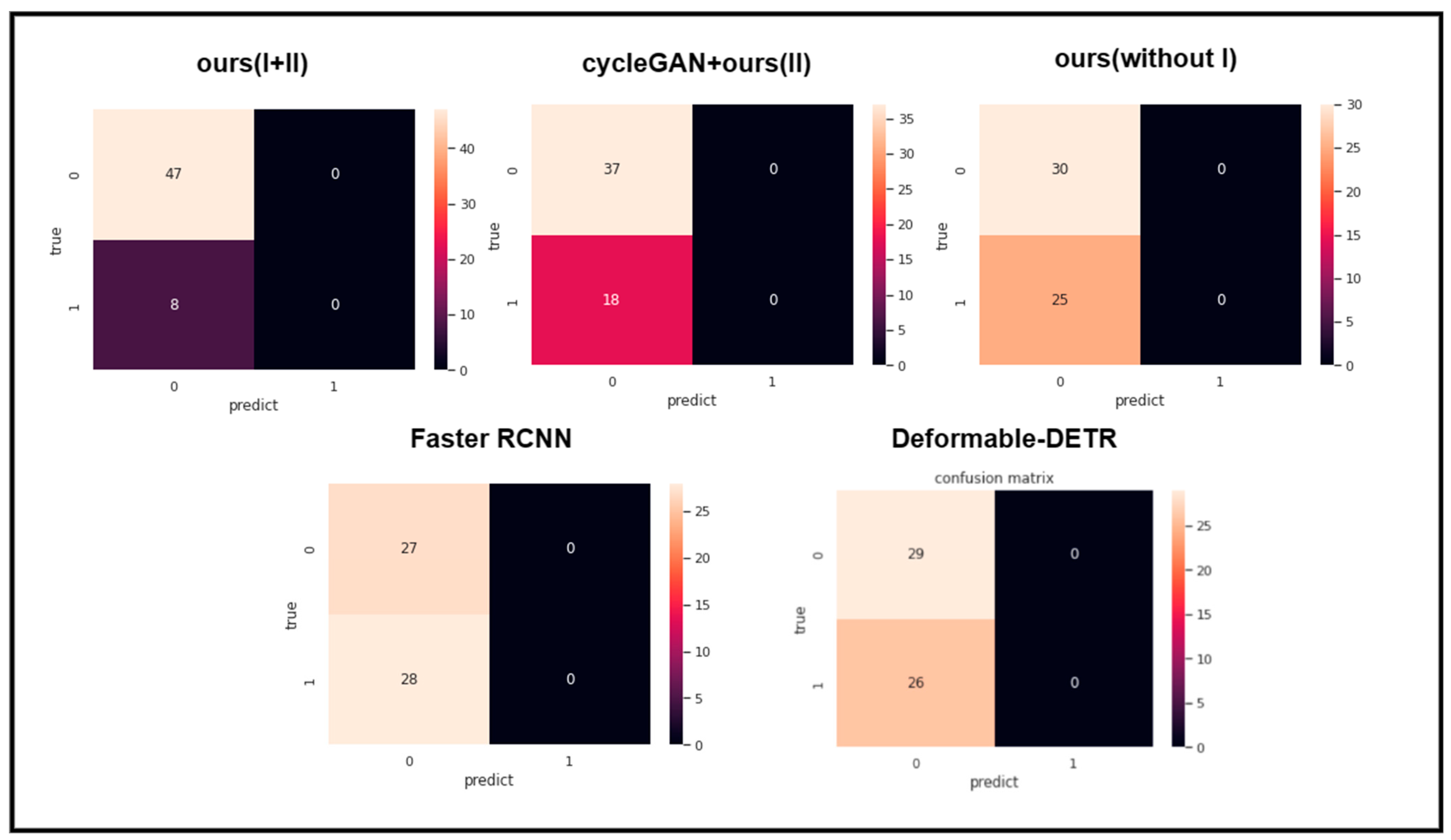
In this experiment, ten low-light images were randomly selected from the dataset. After calculating the statistics for 55 risk factor targets, four different methods were used to detect and verify them. For selection of the ten images, we first randomly selected eight images from among the experimental images. To demonstrate the regional enhancement effect of our dual discriminator on local low illumination images, we specifically added two random local low illumination images. This process ensured that there were at least two local low illumination images in each batch of experimental sets, thus preventing small probability events, such as missing local low illumination images, from occurring throughout the experimental set. In this process, the first confusion matrix of the four combination methods was obtained. Next, we repeated the process for obtaining the confusion matrix seven times. For statistical convenience, we proportionally expanded or reduced the results based on the total number of batch targets and the total number of benchmark targets (55), thereby ensuring that the proportion of results to the total number of benchmark targets was approximately the same as the proportion of results to the total number of batch targets before the change. We then averaged the results eight times to obtain the following average confusion matrix (Figure 9).

Figure 9.
Average confusion matrix. (The figures in the diagram indicate the number of targets related to their respective classifications, and their approximate range is distinguished by color for ease of comprehension.)
The first column in the confusion matrix represents the number of targets predicted to be dangerous targets (0), and the first row in the first column represents the number of targets that are actually dangerous targets (0), namely TP (True Positive) Results. The second row in the first column represents the number of actual non-hazardous targets (1), which are FP (False Positive) results. The second column similarly represents the number of targets predicted as non-hazardous targets (1), and different rows represent whether those targets are actually hazardous targets, namely FN (False Negative) and TN (True Negative) results. Thus, the true aliasing rate (TCr), mean true aliasing rate (mTCr), false aliasing efficiency (FCr), and mean false aliasing efficiency (mFCr) can be expressed by a formula, where n is the number of times the confusion matrix is experimentally obtained. In general, the higher the true obfuscation rate, the lower the false obfuscation rate, which results in a low proportion of targets representing obfuscation, indicating better detection performance:
The mean true confusion rate (mTCr) and mean false confusion rate (mFCr) of eight confusion matrix experiments conducted using the four methods were recorded in a table (Table 1), and the results were presented to two decimal places. As all 55 targets in the experiment were actually dangerous targets (0), we determined that the false confusion rate and true confusion rate combined to approximately 1. In comparison, we found that the second-stage detection model was generally superior to mainstream convolutional networks and that the first stage could overcome the impact of low illumination in the whole or partial region upon detection.

Table 1.
Comparison of the true confusion rate and false confusion rate of the four methods.
5. Conclusions
In this paper, we used a two-stage deep learning model framework to solve the adaptive detection problem for low illumination environments. The entire training process has low requirements for training data and offers good operability and generalization. The experimental results showed that our method can adaptively overcome the impact of low illumination on detection in the first stage, while detection in the second stage remained superior to that of mainstream convolutional detection models without adaptive conversion conditions. By adding adaptive conversion conditions, there was a significant improvement in detection under low illumination. In future work, we plan to combine the algorithm with sensor innovation while also improving the overall robustness of the detection model from other dimensions so that it can maintain good detection performance in various extreme situations.
Author Contributions
Conceptualization, H.W. and B.Y.; methodology, B.Y. and W.W.; software, H.W.; validation, C.Z.; investigation, W.W.; writing—original draft preparation, H.W.; writing—review and editing, C.Z.; funding acquisition, B.Y. All authors have read and agreed to the published version of the manuscript.
Funding
This research was funded by the 2022 Shenyang Science and Technology Plan ‘Jie Bang Gua Shuai’ Key Core Technology Tackling Project (22-316-1-10, Shenyang Bureau of Science and Technology).
Data Availability Statement
Data underlying the results presented in this paper are not publicly available at this time but may be obtained from the authors upon reasonable request.
Conflicts of Interest
The authors declare no conflict of interest.
References
- Jiang, L.; Jing, Y.; Hu, S.; Ge, B.; Xiao, W. Deep Refinement Network for Natural Low-Light Image Enhancement in Symmetric Pathways. Symmetry 2018, 10, 491. [Google Scholar] [CrossRef]
- Saito, K.; Saenko, K.; Liu, M.Y. Coco-funit: Few-shot unsupervised image translation with a content conditioned style encoder. In Computer Vision–ECCV 2020: 16th European Conference, Glasgow, UK, 23–28 August 2020, Proceedings, Part III 16; Springer: Berlin/Heidelberg, Germany, 2020. [Google Scholar]
- Ivan, A.; Pavel, S.; Denis, K.; Alexey, K.; Taras, K.; Aleksei, S.; Sergey, N.; Victor, L.; Gleb, S. Highresolution daytime translation without domain labels. In Proceedings of the IEEE/CVF Conference on Computer Vision and Pattern Recognition, Seattle, WA, USA, 13–19 June 2020. [Google Scholar]
- Ren, S.; He, K.; Ross, G.; Sun, J. Faster r-cnn: Towards real-time object detection with region proposal networks. IEEE Trans. Pattern Anal. Mach. Intell. 2017, 39, 1137–1149. [Google Scholar] [CrossRef] [PubMed]
- Baek, K.; Choi, Y.; Uh, Y.; Yoo, J.; Shim, H. Rethinking the truly unsupervised image-to-image translation. In Proceedings of the IEEE/CVF International Conference on Computer Vision, Montreal, QC, Canada, 11–17 October 2021. [Google Scholar]
- Tian, Z.; Shen, C.; Chen, H.; He, T. Fcos: Fully convolutional onestage object detection. In Proceedings of the 2019 IEEE/CVF International Conference on Computer Vision (ICCV), Seoul, Republic of Korea, 27 October–2 November 2019; pp. 9627–9636. [Google Scholar]
- Okawara, T.; Yoshida, M.; Nagahara, H.; Yagi, Y. Action Recognition from a Single Coded Image. In Proceedings of the IEEE International Conference on Computational Photography, St. Louis, MO, USA, 24–26 April 2020; pp. 1–11. [Google Scholar]
- Wang, C.Y.; Bochkovskiy, A.; Liao, H. Scaled-YOLOv4: Scaling Cross Stage Partial Network. Computer Vision and Pattern Recognition. In Proceedings of the IEEE/cvf Conference on Computer vision and Pattern Recognition, Virtual, 19–25 June 2021. [Google Scholar]
- Nicolas, C.; Francisco, M.; Gabriel, S.; Nicolas, U.; Alexander, K.; Sergey, Z. End-to-end object detection with transformers. In European Conference on Computer Vision; Springer: Berlin/Heidelberg, Germany, 2020; pp. 213–229. [Google Scholar]
- Girshick, R. Fast R-CNN. Computer Science. In Proceedings of the 2015 IEEE International Conference on Computer Vision (ICCV), Santiago, Chile, 7–13 December 2015. [Google Scholar]
- Li, L.; Zhang, P.; Zhang, H.; Yang, J.; Li, C.; Zhong, Y.; Wang, L.; Yuan, L.; Zhang, L.; Hwang, J.; et al. Grounded language-image pre-training. In Proceedings of the International Conference on Machine Learning, Guangzhou China, 18–21 February 2022. [Google Scholar]
- Shao, S.; Li, Z.; Zhang, T.; Peng, C.; Yu, G.; Zhang, X.; Li, J.; Sun, J. Objects365: A large-scale, high-quality dataset for object detection. In Proceedings of the IEEE/CVF International Conference on Computer Vision, Seoul, Republic of Korea, 27 October–2 November 2019; pp. 8430–8439. [Google Scholar]
- Aishwarya, K.; Mannat, S.; Yann, L.; Ishan, M.; Gabriel, S.; Nicolas, C. Mdetr—Modulated detection for end-to-end multi-modal understanding. In Proceedings of the IEEE/CVF International Conference on Computer Vision, Montreal, BC, Canada, 11–17 October 2021. [Google Scholar]
- Zhu, Z.; Xu, Z.; You, A.; Bai, X. Semantically multi-modal image synthesis. In Proceedings of the IEEE/CVF Conference on Computer Vision and Pattern Recognition 2020, Seattle, WA, USA, 14–19 June 2020. [Google Scholar]
- Lore, K.G.; Akintayo, A.; Sarkar, S. LLNet: A Deep Autoencoder Approach to Natural Low-light Image Enhancement. Pattern Recognit. 2017, 61, 650–662. [Google Scholar] [CrossRef]
- Tao, L.; Zhu, C.; Xiang, G.; Li, Y.; Jia, H.; Xie, X. LLCNN: A convolutional neural network for low-light image enhancement. In Proceedings of the 2017 IEEE Visual Communications and Image Processing (VCIP), Suzhou, China, 13–16 December 2018. [Google Scholar]
- Chen, W.; Wenjing, W.; Wenhan, Y.; Jiaying, L. Deep retinex decomposition for low-light enhancement. arXiv 2018, arXiv:1808.04560. [Google Scholar]
- Shangzhe, W.; Jiarui, X.; Yu-Wing, T.; Chi-Keung, T. Deep high dynamic range imaging with large foreground motions. In Proceedings of the European Conference on Computer Vision (ECCV), Munich, Germany, 8–14 September 2018; pp. 117–132. [Google Scholar]
- Jianrui, C.; Shuhang, G.; Lei, Z. Learning a deep single image contrast enhancer from multi-exposure images. IEEE Trans. Image Process. 2018, 27, 2049–2062. [Google Scholar]
- Vaswani, A.; Shazeer, N.; Parmar, N.; Uszkoreit, J.; Jones, L.; Gomez, A.N.; Kaiser, L.; Polosukhin, I. Attention Is All You Need. arXiv 2017, arXiv:1706.03762. [Google Scholar]
- Sun, L.; Wang, K.; Yang, K.; Xiang, K. See clearer at night: Towards robust nighttime semantic segmentation through day-night image conversion. arXiv 2019, arXiv:1908.05868. [Google Scholar]
- Goodfellow, I.; Pouget-Abadie, J.; Mirza, M.; Xu, B.; Warde-Farley, D.; Ozair, S.; Courville, A.; Bengio, Y. Generative Adversarial Nets. Commun. ACM 2020, 63, 139–144. [Google Scholar] [CrossRef]
- Yu, B.; Wei, H.; Wang, W. GAN-Based Day and Night Image Cross-Domain Conversion Research and Application. In Proceedings of the 2022 11th International Conference of Information and Communication Technology, Wuhan, China, 24–26 June 2022; pp. 230–235. [Google Scholar]
- Chen, Y.; Xu, X.; Tian, Z.; Jia, J. Homomorphic latent space interpolation for unpaired imageto-image translation. In Proceedings of the IEEE/CVF Conference on Computer Vision and Pattern Recognition, Long Beach, CA, USA, 15–19 June 2019. [Google Scholar]
- Anoop, C.; Alan, S. Sem-gan: Semanticallyconsistent image-to-image translation. In Proceedings of the 2019 IEEE Winter Conference on Applications of Computer Vision, Waikoloa, HI, USA, 7–11 January 2019. [Google Scholar]
- Yunjey, C.; Minje, C.; Munyoung, K. Stargan: Unified generative adversarial networks for multi-domain image-to-image translation. In Proceedings of the IEEE Conference on Computer Vision and Pattern Recognition 2018, Salt Lake City, UT, USA, 18–23 June 2018. [Google Scholar]
- Lin, J.; Chen, J.; Xia, Y.; Liu, S.; Qin, T.; Luo, J. Exploring explicit domain supervision for latent space disentanglement in unpaired image-to-image translation. arXiv 2019, arXiv:1902.03782. [Google Scholar] [CrossRef] [PubMed]
- Luigi, M.; Andrea, Z. Semantically adaptive image-to-image translation for domain adaptation of semantic segmentation. arXiv 2020, arXiv:2009.01166. [Google Scholar]
- Ali, J.; Lucy, C.; Phillip, I. On the ”steerability” of generative adversarial networks. arXiv 2020, arXiv:1907.07171. [Google Scholar]
- Peilun, L.; Xiaodan, L.; Daoyuan, J.; Eric, P.X. Semantic-aware grad-gan for virtual-to-real urban scene adaption. arXiv 2018, arXiv:1801.01726. [Google Scholar]
- Tian, X.; Wang, L.; Ding, Q. Overview of image semantic segmentation methods based on deep learning. J. Softw. 2019, 30, 440–468. [Google Scholar]
- Hoffman, J.; Tzeng, E.; Park, T.; Zhu, J.Y.; Isola, P.; Saenko, K.; Efros, A.; Darrell, T. CyCADA: Cycle-Consistent Adversarial Domain Adaptation. In Proceedings of the International Conference on Machine Learning, Stockholm, Sweden, 10–15 July 2018. [Google Scholar]
- Dai, X.; Chen, Y.; Yang, J.; Zhang, P.; Yuan, L.; Zhang, L. Dynamic detr: End-to-end object detection with dynamic attention. In Proceedings of the IEEE/CVF International Conference on Computer Vision (ICCV), Montreal, BC, Canada, 11–17 October 2021; pp. 2988–2997. [Google Scholar]
- Dai, X.; Chen, Y.; Xiao, B.; Chen, D.; Liu, M.; Yuan, L.; Zhang, L. Dynamic head: Unifying object detection heads with attentions. In Proceedings of the IEEE/CVF Conference on Computer Vision and Pattern Recognition, Virtual, 19–25 June 2021; pp. 7373–7382. [Google Scholar]
- Marco, T.; Umberto, M.; Gianluca, A.; Pietro, Z. Unsupervised domain adaptation for mobile semantic segmentation based on cycle consistency and feature alignment. Image Vis. Comput. 2020, 95, 103889. [Google Scholar]
- Yang, X.; Xu, Z.; Luo, J. Towards perceptual image dehazing by physics-based disentanglement and adversarial training. In Proceedings of the AAAI Conference on Artificial Intelligence, New Orleans, LI, USA, 2–7 February 2018. [Google Scholar]
- Wang, Y.; Zhang, X.; Yang, T.; Sun, J. Anchor detr: Query design for transformer-based detector. Proc. AAAI Conf. Artif. Intell. 2022, 36, 2567–2575. [Google Scholar] [CrossRef]
- Sun, Z.; Cao, S.; Yang, Y.; Kris, K. Rethinking transformer-based set prediction for object detection. In Proceedings of the IEEE/CVF International Conference on Computer Vision, Montreal, BC, Canada, 11–17 October 2021. [Google Scholar]
- Hamid, R.; Nathan, T.; JunYoung, G.; Amir, S.; Ian, R.; Silvio, S. Generalized intersection over union: A metric and a loss for bounding box regression. In Proceedings of the IEEE/CVF Conference on Computer Vision and Pattern Recognition, Long Beach, CA, USA, 16–17 June 2019; pp. 658–666. [Google Scholar]
Disclaimer/Publisher’s Note: The statements, opinions and data contained in all publications are solely those of the individual author(s) and contributor(s) and not of MDPI and/or the editor(s). MDPI and/or the editor(s) disclaim responsibility for any injury to people or property resulting from any ideas, methods, instructions or products referred to in the content. |
© 2023 by the authors. Licensee MDPI, Basel, Switzerland. This article is an open access article distributed under the terms and conditions of the Creative Commons Attribution (CC BY) license (https://creativecommons.org/licenses/by/4.0/).

