Abstract
The generation of structured grids on bounded domains is a crucial issue in the development of numerical models for solving differential problems. In particular, the representation of the given computational domain through a regular parameterization allows us to define a univalent mapping, which can be computed as the solution of an elliptic problem, equipped with suitable Dirichlet boundary conditions. In recent years, Physics-Informed Neural Networks (PINNs) have been proved to be a powerful tool to compute the solution of Partial Differential Equations (PDEs) replacing standard numerical models, based on Finite Element Methods and Finite Differences, with deep neural networks; PINNs can be used for predicting the values on simulation grids of different resolutions without the need to be retrained. In this work, we exploit the PINN model in order to solve the PDE associated to the differential problem of the parameterization on both convex and non-convex planar domains, for which the describing PDE is known. The final continuous model is then provided by applying a Hermite type quasi-interpolation operator, which can guarantee the desired smoothness of the sought parameterization. Finally, some numerical examples are presented, which show that the PINNs-based approach is robust. Indeed, the produced mapping does not exhibit folding or self-intersection at the interior of the domain and, also, for highly non convex shapes, despite few faulty points near the boundaries, has better shape-measures, e.g., lower values of the Winslow functional.
Keywords:
physics-informed neural networks; planar domains; quasi-interpolation; spline parameterization MSC:
65D07; 65D17; 65N50
1. Introduction
Computer-Aided Design (CAD) systems only provide the boundary representation of the given computational domain, but in order to perform numerical simulation, a representation of the interior is often necessary. While many techniques based on the use of triangulations, see, e.g., [1,2], are available for unstructured grids, the generation of structured grids via analysis-suitable parameterizations is still challenging, especially when the considered domains are not convex. The main requirement is to obtain a bijective, and, hence, a folding-free, mapping defined on the reference domain which provides a description of the considered computational domain ,
The image of a uniform, Cartesian grid in under the mapping is a curvilinear, boundary conforming grid in the physical domain , with a uniform topological structure, i.e., same number of vertices, cells, neighboring cells, and so on. When the final goal is to perform numerical simulation on , by using the pull-back of the mapping , the considered differential problem can be efficiently carried out on the parametric domain , see, e.g., [3,4]. Hence, the invertibility requirement imposed on becomes fundamental.
From the computational point of view, the cheapest techniques to construct rely on transfinite interpolation, such as the Coons patches [5] and the spring model [6]. Unfortunately, such techniques fail to produce a folding-free when the assayed domain has a complex shape or is not convex. Therefore, other more advanced methods, based on the use of specific functionals that control the quality of the obtained parameterization [7,8,9], are adopted, together with the use of conformal and harmonic mappings which intrinsically ensure a high-quality result, see, e.g., [10,11,12]. In the present paper, an approach based on the so-called Elliptic Grid Generation (EGG) methods is proposed. Indeed, EGG methods are particularly suitable for the current setting as only a description of the boundary of is required. The mapping is constructed as the solution of a system of elliptic PDEs defined on subject to Dirichlet boundary conditions, i.e., . Moreover, the bijectivity of is guaranteed as long as the numerical accuracy is good enough and the produced curvilinear grid in is smooth, which results in small truncation errors when domain methods are employed to perform numerical simulation on the considered . We refer to [13,14,15] and references therein for a comprehensive review of EGG techniques and their recent applications. When the shape of is rather challenging or not convex, a segmentation in subdomains, called patches, with easier shape is usually advised and the description of is thus obtained as an atlas whose charts are the individual bijective parameterizations for each patch. The main challenges of such approach consist in the identification of a suitable segmentation technique [16,17,18,19] and in the smooth transition between the patches [20,21].
In the last two decades, machine learning and deep learning techniques have started to play an active role in the setting up of new methods for the numerical solution of PDEs [22,23,24]. In particular, Physics-Informed Neural Networks (PINNs) [25,26,27] have emerged as an intuitive and efficient deep learning framework to solve PDEs, carrying on the training of a neural network by minimizing the loss functional which incorporates the PDE itself, informing the neural network about the physical problem to be solved.
In the proposed method, the final parameterization is obtained by means of quasi-interpolation; a local approach to construct approximants to given functions or data with full approximation order. Spline quasi-interpolants (QI) are usually defined as linear combination of locally supported basis functions forming a convex partition of unity. The coefficients of such a linear combination, called functionals, can be defined in different ways by taking into account the function evaluations, its derivative information or its integral values, see for example [28,29,30,31]. In the present paper we rely on the QI-Hermite technique introduced in [32], which is a differential type QI used together with PINNs to produce a single-patch parameterization methodology. In particular, a suitable PINNs architecture and loss function will be presented to fit within the EGG methods framework. Finally, the use of the QI operator will allow us to produce a robust output regardless from the input shape of without requiring a preliminary segmentation of the computational domain. The main contribution of this work consists of introducing a novel algorithm to compute a single patch planar domain parameterizations. In particular:
- The discrete description of the computational domain is achieved by using PINNs.
- The continuous representation of the computational domain is then obtained by using a suitable QI operator which provides a spline parameterization, i.e., a continuous description, of the desired smoothness.
The paper is organized as follows. Section 2 summarizes the main concepts about quasi-interpolation and PINNs; Section 3 is devoted to the pipeline description of our method; then numerical examples are presented in Section 4 in order to analyze the quality of the proposed method and in Section 5 a suitable post-processing step is described in order to handle more challenging benchmarks. Finally, Section 6 draws some conclusive remarks.
2. Preliminaries
Let us summarize the main concepts of the adopted QI scheme together with the basics ideas of the PINNs model.
In the following, the spline Hermite QI introduced in [32] is considered. In particular, its version based on the derivative approximation presented in [33] will be employed. For the univariate case, let be the space of splines with degree p and associated extended knot vector T defined in the reference domain ; , with and . A spline can be represented by using the standard B-spline basis , defined on T:
The unknown coefficient vector can be computed by solving local linear systems of dimension . The derivatives are approximated by using a symmetric finite difference scheme and, hence, the entries of the vector are a linear combination of the function to be approximated.
The tensor product formulation of the scheme can be easily derived; a spline s in the space , can be written as,
Setting and , s can be expressed compactly as,
with tensor product B-spline basis. The approximation order of the scheme is maximal if the approximation order of the derivatives is bigger than . For more technical details we refer to [34].
PINNs are a class of learning algorithms used to solve problems involving PDEs [25,27]. An L-layers neural network (typically, a feedforward neural network) is an architecture consisting of neurons at the ℓ-th layer with and . Let and be, respectively, the matrix of weights and the vector of bias at the layer ℓ. The net then can be generally described with the following scheme:
with a non linear activation function. The constructed net is trained to compute the (approximate) solution of the involved PDE, and the training phase is carried out by minimizing a suitable loss functional which takes into account the given boundary conditions along with the so-called residual term. For a theoretical investigation of the convergence properties and stability analysis related to PINNs, see, e.g., [35,36].
3. The Method
The aim of the proposed EGG-based method consists in computing a parameterization of a given planar domain by solving the following system,
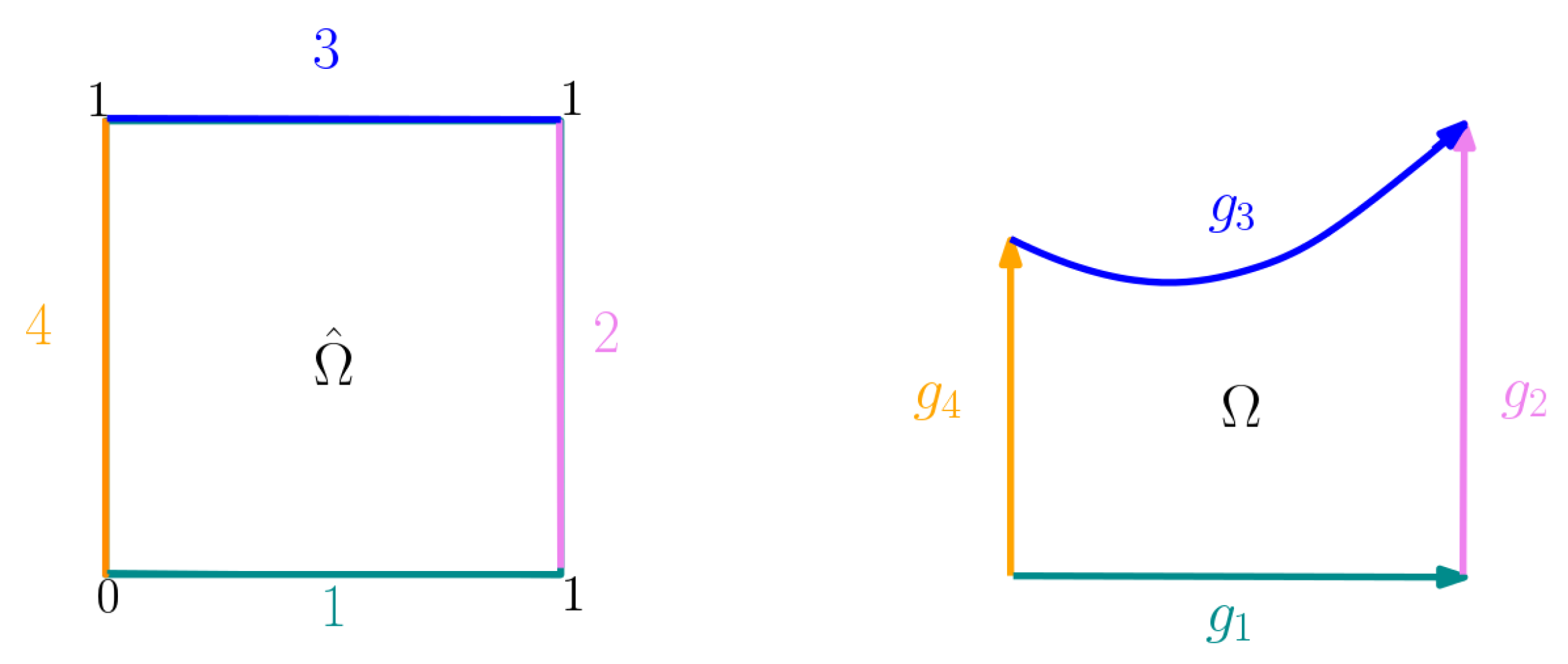
where the boundary of the domain can be described as the non-overlapping union of four boundary curves and the Dirichlet boundary conditions are given by the functions invertible parameterizations of the boundary curves, according to the scheme exemplified in Figure 1.

Figure 1.
Scheme of the applied Dirichlet boundary conditions.
A net consisting of layers with and for , neurons is constructed. Then, the provided output is an approximate solution of problem (3) which depends on a set of parameters . The following functional is minimized,
where collects uniformly sampled parameters corresponding to points located on the four boundary curves, while is a set of uniformly sampled points inside . More precisely, the loss functional in (4) consists of the terms,
where the first term corresponds to the mean squared error between the predicted location of the boundary points and the assigned points given by the boundary conditions, while the second term is called residual term and relates directly to the differential problem (this explains why the neural network is called physics informed). Its computation is carried on by means of automatic differentiation, a procedure to compute derivatives with respect to sample batches based on backpropagation technique [37], nowadays implemented in most of Deep Learning packages, such as Tensorflow [38], PyTorch [39], and Jax [40]. The parameter w in (4) is determined via thresholding on the proximity of the interior points to the boundaries; if , otherwise . Training is performed on an Intel(R) Core(TM) i7-9800X processor running at 3.80 GHz using 31 GB of RAM along with a GeForce GTX 1080 Ti GPU unit by using the Tensorflow package. The training phase firstly is carried on for 5000 epochs with the Adam optimizer [41] with learning rate , and afterwards for 10,000 epochs with the L-BFGS-B algorithm [42], following the method originally proposed in [25] to have (empirical) convergence guarantees. The weights are initialized under the Xavier initialization method [43]. The adopted non-linear activation function for each layer is the hyperbolic tangent tanh. Given different initial , it is observed that PINNs may converge to different solutions, see, e.g., [44,45]. Hence, our experiments are performed 10 times, changing the initial random seed and producing 10 approximate solutions. Since there is no guarantee of a unique solution, as a non-convex optimization problem is solved by minimizing (4), the selected which is retained corresponds to the solution achieving the smallest residual term. The PINNs code outputs the predicted evaluation of at points inside . At this stage, a quasi-interpolant splines is constructed by adopting Formula (2).
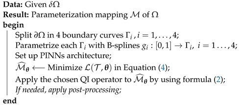
The generation pipeline, outlined in Algorithm 1, can be summarized as follows:
- The boundary is split into 4 pieces , for , by performing for example knot-insertion.
- Each is then parametrized as a Bspline curve .
- PINNs are trained to minimize the loss functional in Equation (4) over a set of boundary points and over the Laplace equation.
- The trained network represents an approximation of the sought parameterization map .
- Uniformly spaced grid points are generated in and mapped by to .
- A continuous spline approximation of is obtained by using a Hermite Quasi-Interpolation operator (QI).
| Algorithm 1 Pseudo-code for the proposed algorithm |
 |
4. Numerical Examples
In this section, some numerical experiments are performed on specific planar shapes which are typical benchmarks considered in assessing the quality of the produced parameterization, see, e.g., [7,15]. The experiments have been chosen with increasing complexity. Firstly a fully symmetric and convex domain is assayed. Then, for the second example, is a non-convex and non-symmetric domain, but it can be obtained by a simple deformation of . The third benchmark is a slightly non-convex domain, while the fourth and fifth examples consider highly non convex and non symmetric shapes. Moreover, some comparisons are shown with respect to two techniques suitable for 4-sided shaped domains which only need a description of the boundary, Coons patches and the inpaint technique, which is computing a harmonic mapping as introduced in (1), such that
with boundary conditions given as in Problem 3. This mapping is computed by approximating the discrete Laplace operator by finite difference formulas. John D’Errico (2023). inpaint_nans (https://www.mathworks.com/matlabcentral/fileexchange/4551-inpaint_nans, accessed on 16 April 2023), MATLAB Central File Exchange. The evaluation of the three techniques is performed by checking if the fundamental bijectivity requirement (’Bij’) is satisfied, namely, the determinant of the mapping should always be different from zero and never change sign. Then, the quality of the produced parameterization is also checked by computing the following functional,
with J denoting the Jacobian matrix of the mapping .
Expression (5) is known as the Winslow functional, see, e.g., [46] and in order to have a parameterization which is as conformal as possible, i.e., it should be almost a composition of a scaling and a rotation matrix, the best value for W should be 2. Note that, in the specific settings, having a good value for W is an additional property but it is not a necessity, as no additional constraints are imposed to guarantee the minimal achievable W.
4.1. Circle
As first example, a unit circle is considered. The boundary is sampled with 30 points on every , and the final residual term value is . The results with the three approaches are shown in Figure 2, where from top to bottom, on the left column, the distribution of the physical points inside is shown and on the right column, the parametric lines of the computed parameterizations are plotted, for Coons, Inpaint, and Pinns methods, respectively.
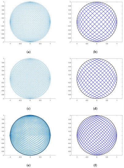
Figure 2.
Circular domain. (a) Points generated via Coons; (b) Linear parameterization with Coons) (c) Points generated via inpaint; (d) Linear parameterization with inpaint; (e) Points with PINNs; and (f) PINNs-QI parameterization.
We remark that in this case the resulting parameterization is singular for all the methods at the image of the four corners of and the considered shape is not particularly challenging, but this example is interesting for symmetry reasons and for visually appreciating how the three methods generate points inside the physical domain . Table 1 collects the evaluation results for this example. All the methods provide a bijective mapping, and, as expected, the values for W are very close to the theoretical optimum.

Table 1.
Circle-shaped domain evaluation.
4.2. Wedge-Shape
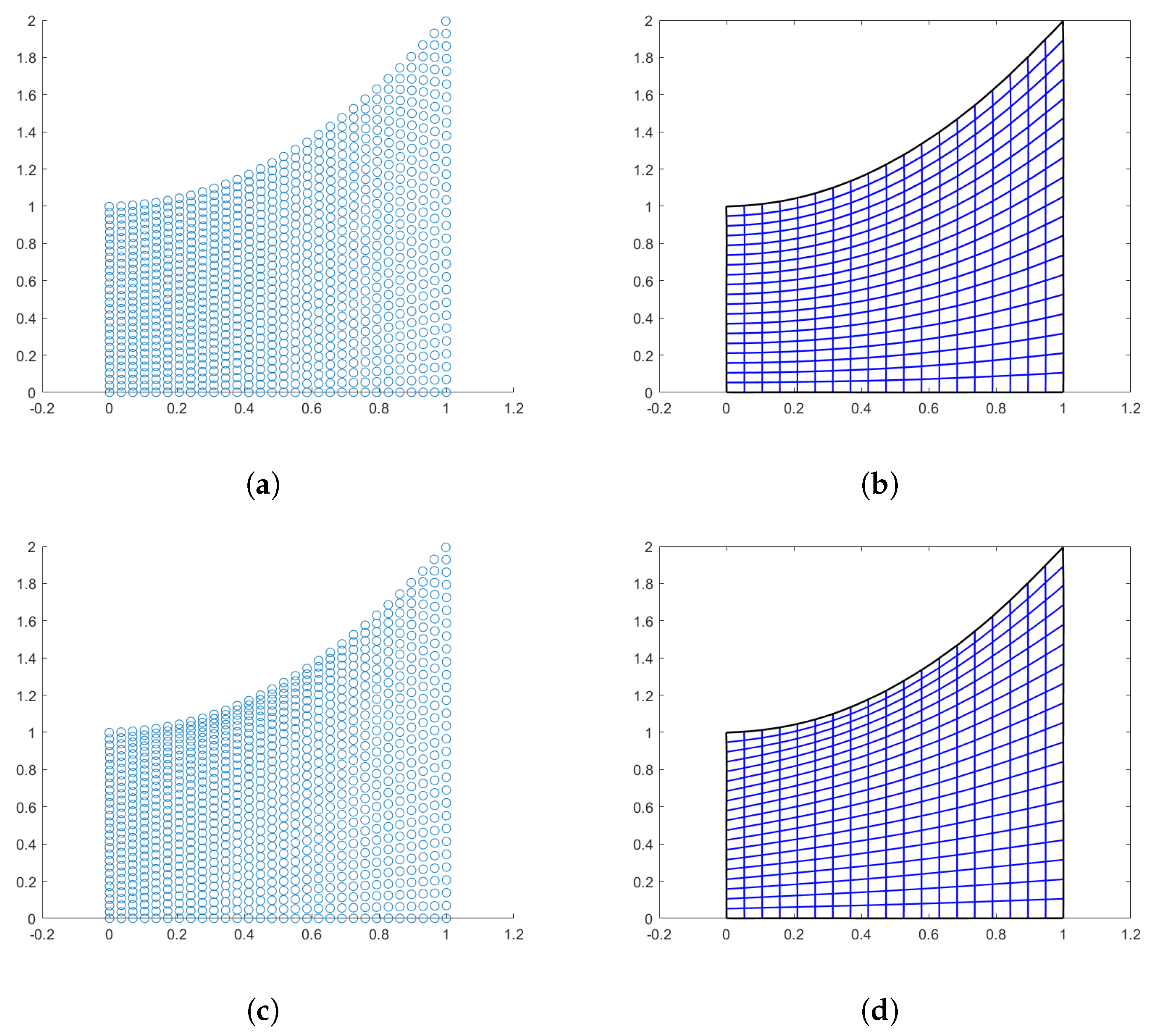
The second example shows a wedge-shaped domain, and the results are presented in Figure 3. In this case, 60 points per boundary curve are sampled and the final accepted mapping for the proposed approach has . All the three considered approaches perform well, as also indicated in Table 2.
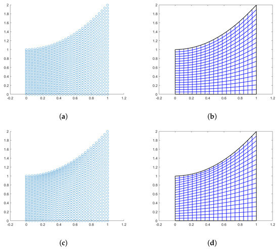

Figure 3.
Wedge-shaped domain. (a) Points generated via Coons; (b) Linear parameterization with Coons; (c) Points generated via inpaint; (d) Linear parameterization with inpaint; (e) Points with PINNs; and (f) PINNs-QI parameterization.

Table 2.
Wedge-shaped domain evaluation.
4.3. Quarter-Annulus-Shaped Domain
The next example is a quarter-annulus-shaped domain, with boundary curves expressed as B-splines with knot vectors (KV) and and control points as given in Table 3, for .

Table 3.
Descriptors for the quarter-annulus shaped boundary curves.
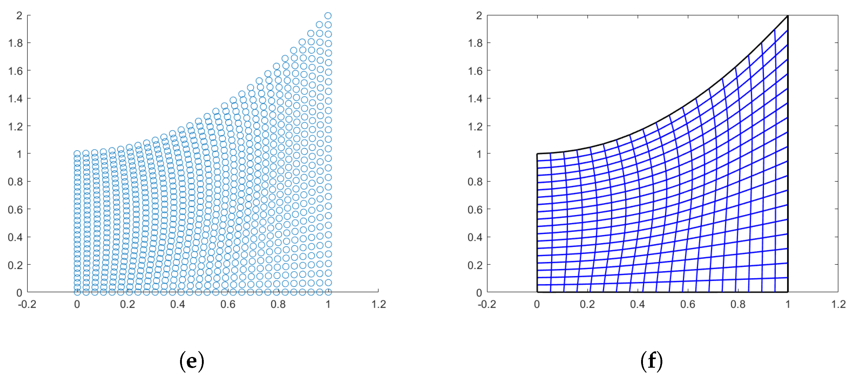
In Figure 4, we see the results obtained by the three methods with using linear splines interpolation for the Coons and Inpaint case, while using a quadratic quasi-interpolant spline for the PINNs method (). Regarding the evaluation of this domain, the linear mapping Jacobian matrix results very ill conditioned, moreover, since and are cubic B-spline curves, it seems more pertinent to construct a cubic parameterization where the used knots for the boundary curves are a refinement of the vectors and . Therefore, Table 4 shows the results obtained by adopting the same QI operator of bi-degree 3 on the given sample points provided by the three methods. The obtained mapping is bijective in all the three cases and the value for the Winslow functional is almost optimal as well.
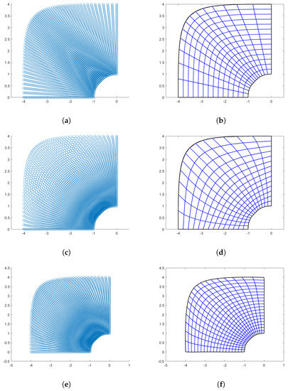
Figure 4.
Quarter-annulus domain. (a) Points generated via Coons; (b) Linear parameterization with Coons; (c) Points generated via inpaint; (d) Linear parameterization with inpaint; (e) Points generated with PINNs; and (f) PINNs-QI parameterization.

Table 4.
Quarter circle-shaped domain evaluation.
4.4. Hourglass-Shaped Domain
The next example is an hourglass-shaped domain with boundary curves given by cubic B-splines defined on the knot vector for and with corresponding control points reported in Table 5.

Table 5.
Control points for the hourglass shaped domain.
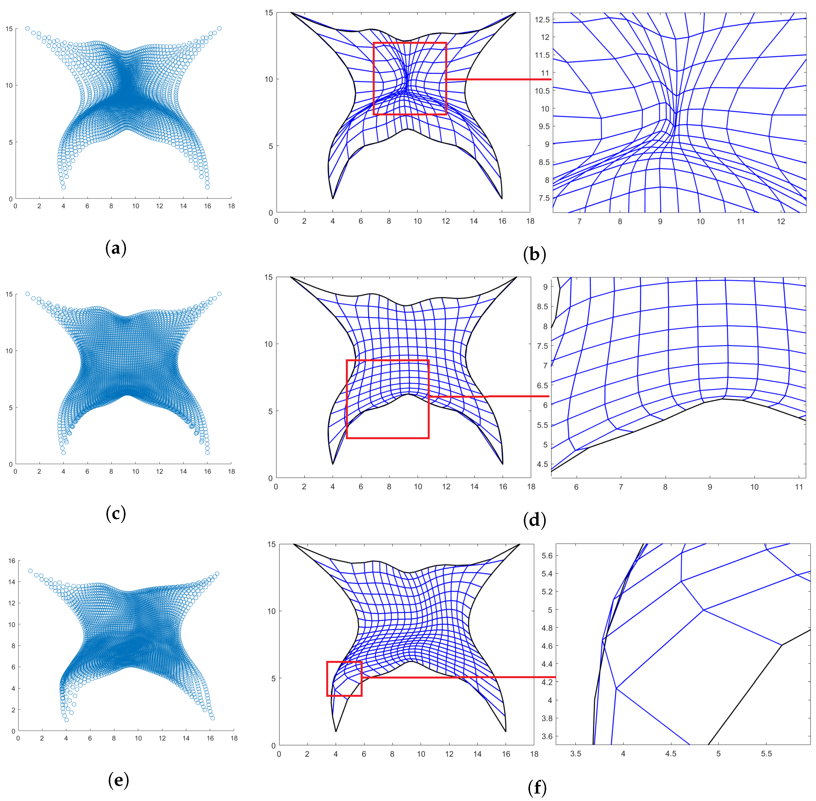
In Figure 5, the hourglass-shaped domain is parametrized by using the three different techniques. On the first row the linear parameterization generated via Coons patches is shown. This parameterization although bijective, as highlighted in the zoomed frame, Figure 5b, and by the fact that its determinant is always strictly positive, presents highly distorted quadrilaterals in the center. On the second row, the parameterization produced by the Inpainting results to be singular, see Figure 5d. At the right boundary, the mapping fails to satisfy the prescribed boundary conditions. Finally, on the last row of Figure 5, the parameterization obtained with the proposed approach is shown. In this case, . In particular, since at the right boundary the produced quadrilaterals look slightly distorted, and the obtained mapping is no longer orientation-preserving, i.e., its determinant is changing sign, in order to improve the quality, a post-processing step, fully described in the next section, is added to the pipeline of the method.
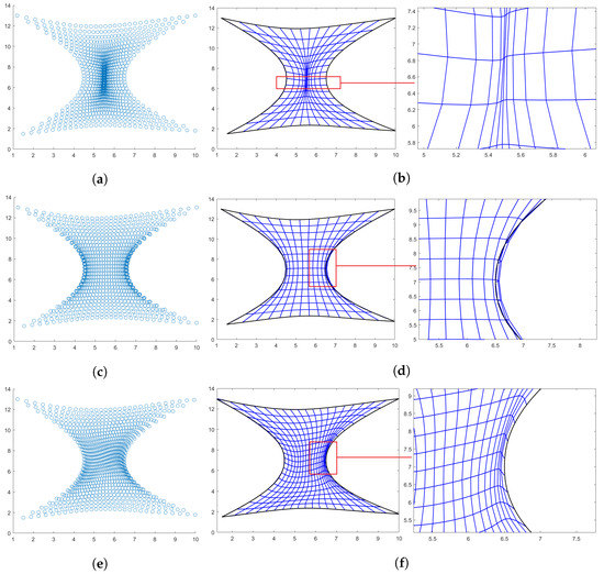
Figure 5.
Hourglass-shaped domain. (a) Points generated via Coons; (b) Linear parameterization with Coons and zoom in; (c) Points generated via inpaint; (d) Linear parameterization with inpaint and zoom in (e) Points generated via PINNs; and (f) PINNs-QI parameterization and zoom in.
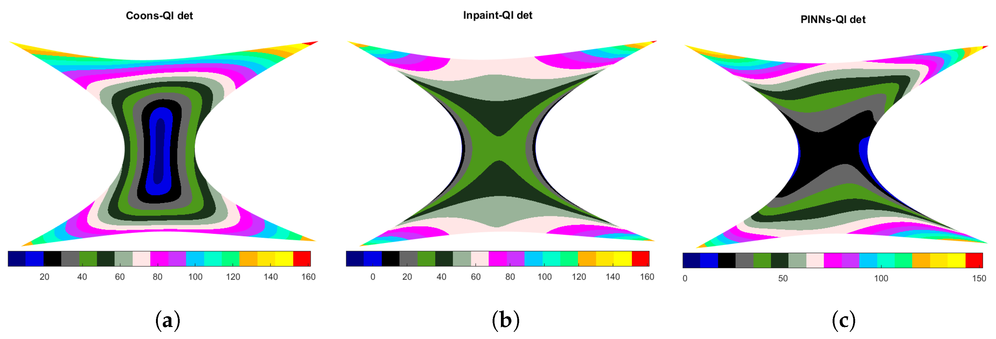
Furthermore, in this case, since the boundary curves are cubic B-splines, in order to exactly reproduce , a bicubic QI spline is constructed on the given sample points for all the three methods. Table 6 reports the results. Moreover, in order to make clearer the behavior of the mapping, a surface plot of the determinant of the Jacobian matrix is also shown for all the three methods in Figure 6. Note that the high values for the should not cause too much concern, as they occur only at the corners of the domain, where the influence of such strong features reflects in high curvature of the produced mapping.

Table 6.
Hourglass-shaped domain evaluation.

Figure 6.
Determinant of the Jacobian matrix for the bicubic parameterization. (a) Method: Coons-QI; (b) Method: Inpaint-QI; and (c) Method: PINNs-QI.
4.5. Butterfly-Shaped Domain
The last example is a more challenging planar domain resembling a butterfly. This domain presents very sharp features which makes it a hard shape to parametrize especially near the four corners. The parameterization of the four boundary curves is realized with cubic B-spline functions with knot vectors, and and control points, as reported in Table 7.

Table 7.
Control points for the butterfly-shaped domain.
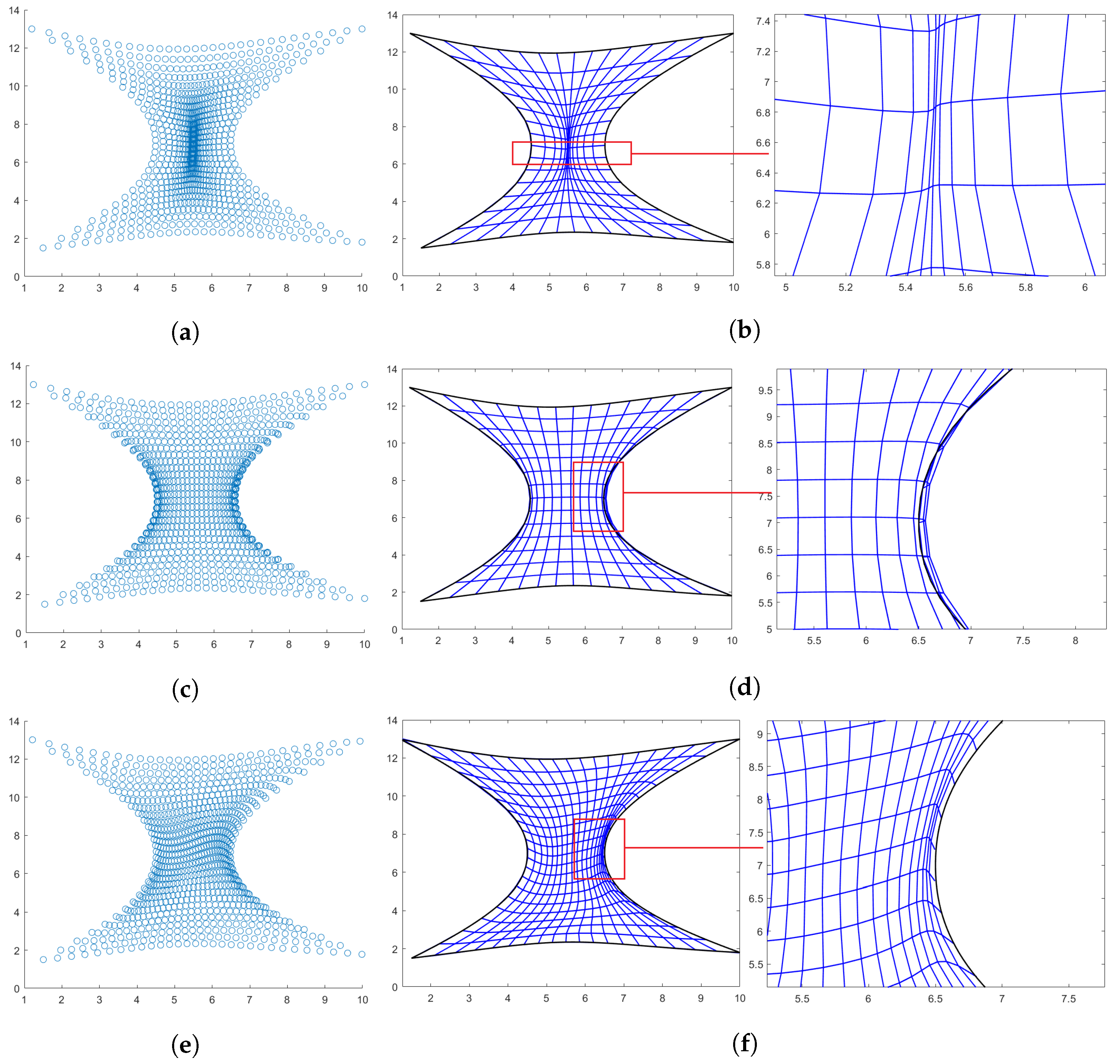
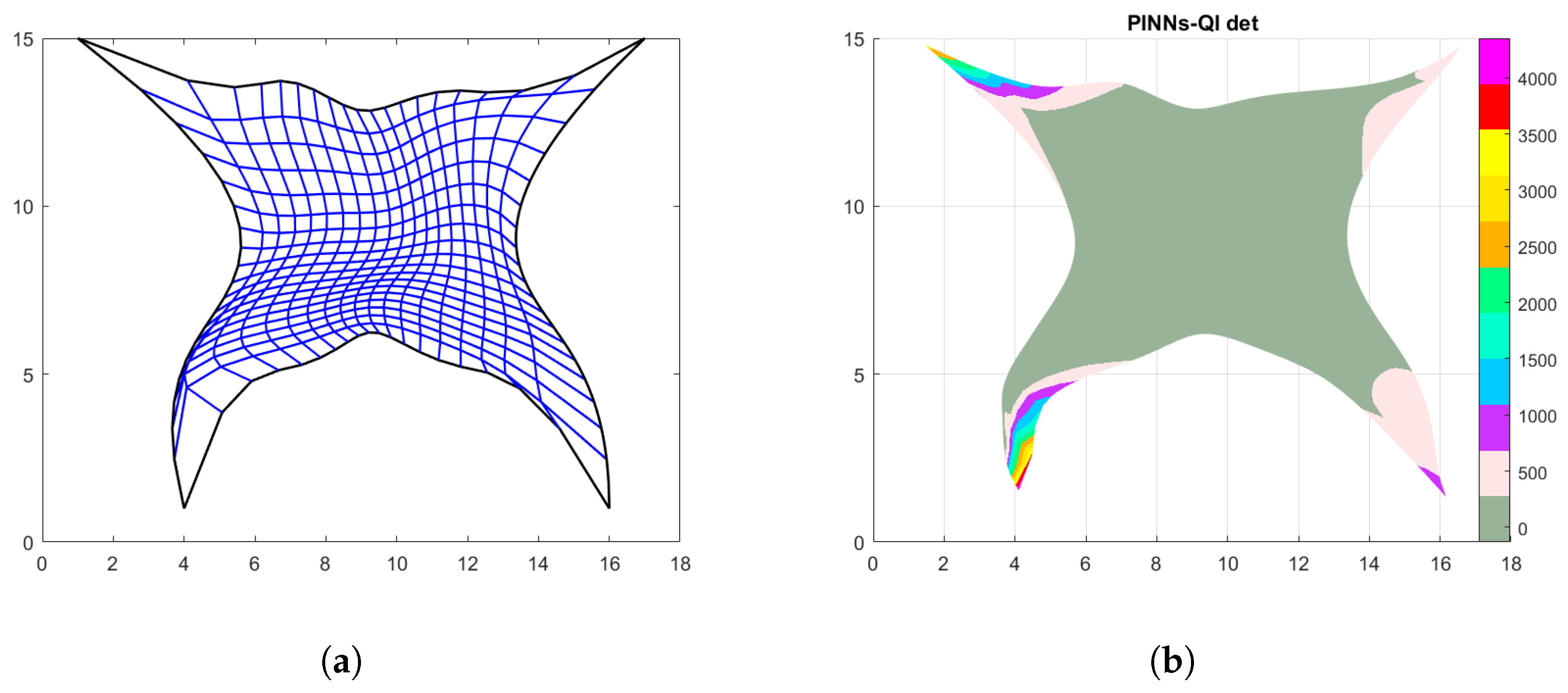
The results obtained with the three methods are shown in Figure 7. None of the methods provides a bijective mapping due to some folding in the center for the Coons patches method and near the south boundary curve for the Inpaint technique. About PINNs () the main issues occur near the left-side boundary curve as the accuracy of the constructed net seems to become poorer near this side of the domain. Otherwise, everywhere else, inside , the produced mapping results perfectly injective. As in the hourglass-shaped domain, to have an exact boundary representation, a cubic QI spline is constructed for all the three methods. Due to the presence of self-intersections though, in some cases, the results for the Winslow functional are equal to ∞, see Table 8.
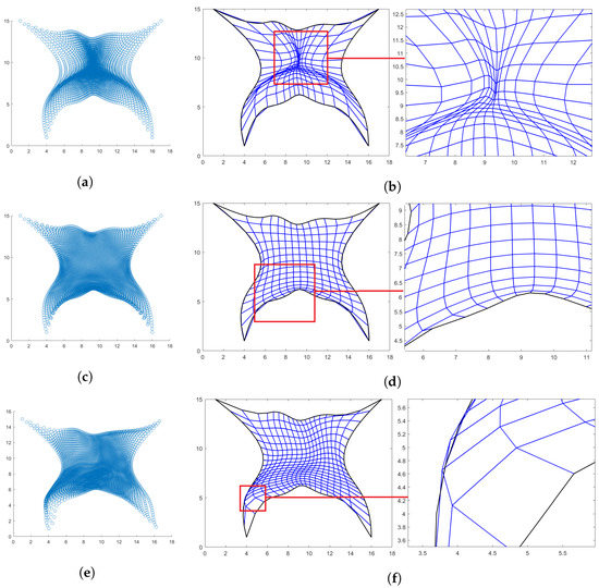
Figure 7.
Butterfly-shaped domain. (a) Points generated via Coons; (b) Linear parameterization with Coons and zoom-in; (c) Points generated via inpaint; (d) Linear parameterization with inpaint and zoom-in; (e) Points generated with PINNs; and (f) PINNs-QI parameterization and zoom-in.

Table 8.
Butterfly-shaped domain evaluation.
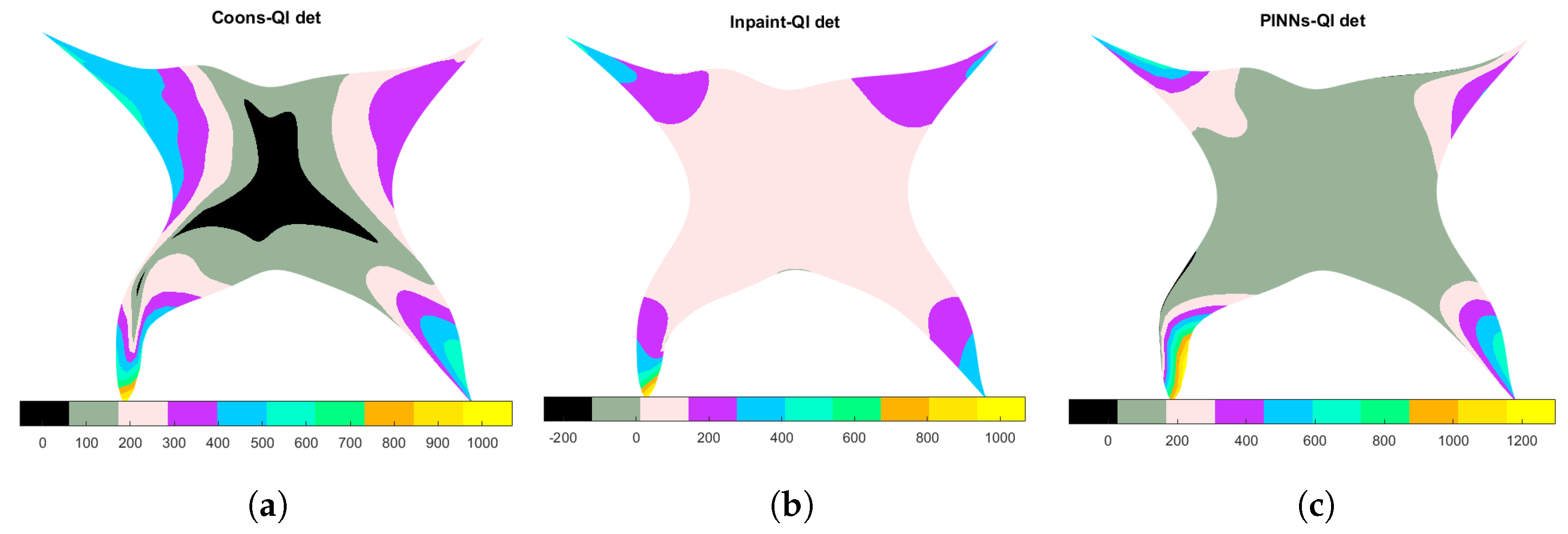
For the PINNs-QI method, although the mapping is not bijective as well, this happens in a very narrow stripe near the left boundary and, also thanks to the regularization provided by the QI, the Winslow functional result is not spoiled. Furthermore, to give a better idea where the mapping fails to be bijective, in Figure 8 the , obtained with the three methods, is plotted as a surface. As for the previous example, the high values for the occur only at specific areas near the corners of the domain.

Figure 8.
Determinant of the Jacobian matrix for the obtained parameterization. (a) Method: Coons; (b) Method: Inpaint; and (c) Method: PINNs-QI.
5. Post-Processing Correction
In order to improve the obtained parameterization when it is not orientation-preserving or when it is not bijective, we rely on the ability of the adopted QI to provide a correction in the following sense. In particular, the hourglass-shaped domain and the butterfly-shaped domain are the cases addressed here. For the first case, as is shown in the zoomed-in frame of Figure 5f and in Figure 6c, the Jacobian of the produced mapping is changing sign near the right-most side of . Hence, the second to last list of physical points outputted by the PINNs code is deleted and regarding the parameter domain, the corresponding parameters are also deleted, producing therefore a non-uniform grid near the right edge. The determinant of the Jacobian matrix of the new mapping ranges between and , obviously the highest values occur at the right corners of the physical domain, as the produced quadrilateral cells are bigger. Furthermore, the value for the Winslow functional slightly increases to , but this is not a significant price to pay to obtain an orientation-preserving mapping. These results are reported in the last row of Table 6 and the final parameterization with the determinant of its Jacobian matrix is shown in Figure 9.
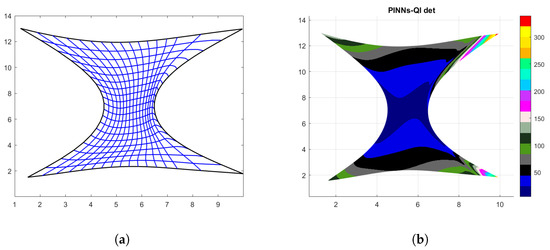
Figure 9.
Correction output. (a) PINNS-QI parameterization after post-processing; and (b) Determinant of J for the post-procecessed mapping.
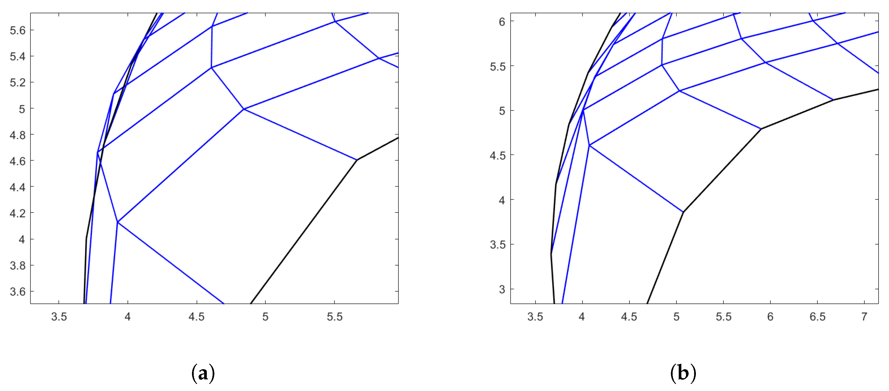
Regarding the butterfly-shaped domain, the main issues occur on the left edge of , see Figure 8c and Figure 10a and also at top edge. Therefore, the faulty physical points are removed, as well as their corresponding parameters in , and the obtained results can be visually appreciated in Figure 10b and Figure 11. The new values for varies between and and the Winslow functional is . These results are also reported in the last row of Table 8.
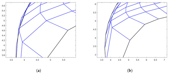
Figure 10.
Comparison before and after post-processing. (a) Zoom-in where there is no injectivity; and (b) Zoom-in after the post-processing correction.
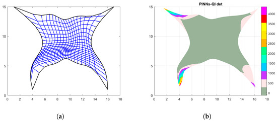
Figure 11.
Results after the post-processing correction. (a) PINNs-QI parameterization after post-processing; and (b) Determinant of the Jacobian matrix after post-processing.
6. Conclusions
In the present paper we have shown how PINNs-driven methods can be profitably used to construct a parameterization of a planar domain by only knowing its boundary representation. In more detail, once an internal set of physical points is obtained, quasi-interpolation is applied to generate a suitable spline parameterization of the given domain. Several planar shapes have been considered with increasing complexity and compared to existing techniques, such as Coons patches and EGG-based methods, needing only the description of the boundary of the computational domain; the obtained results show that this approach is promising. In particular, from the conducted experiments is evident how for symmetric and slightly non-convex domains, all the considered approaches perform well by producing a bijective parameterization which also achieves an almost optimal value for W in all the cases. Regarding more complex shapes, i.e., non-symmetric and highly non-convex domains all the methods exhibit evident faults. Nevertheless, the PINNs-based approach is more robust than the one based on Coons patches, as the produced interior points never allow for folding or self-intersection of the mapping. Regarding the Inpaint technique, being also an EGG method, and, hence, driven by a similar approach, the results are more alike. The main difference in this case lies in the value for W; this is very similar for less complex shapes and much worse for the Inpaint technique when highly non convex domains are analyzed. Future work will be devoted to the study of more sophisticated loss functionals for the considered purpose by trying to achieve bijective mappings that have low distortions, see, e.g., [47,48] and to the extension to the non-planar case.
Author Contributions
Conceptualization, F.M. and M.L.S.; methodology, F.M. and M.L.S.; software, G.A.D. and A.F.; validation, G.A.D. and A.F.; writing—Review and editing, A.F., G.A.D., M.L.S. and F.M. All authors have read and agreed to the published version of the manuscript.
Funding
The research of Antonella Falini was funded by PON Ricerca e Innovazione 2014-202 FSE REACT-EU, Azione IV.4 “Dottorati e contratti di ricerca su tematiche dell’innovazione” CUP H95F21001230006. The research of Francesca Mazzia is funded under the National Recovery and Resilience Plan (NRRP), Mission 4 Component 2 Investment 1.4—Call for tender No. 3138 of 16 December 2021 of Italian Ministry of University and Research funded by the European Union—NextGenerationEU, Project code: CN00000013, Concession Decree No. 1031 of 17 February 2022 adopted by the Italian Ministry of University and Research, CUP: H93C22000450007, Project title: “National Centre for HPC, Big Data and Quantum Computing”. The research of Maria Lucia Sampoli is co-funded by European Union—Next Generation EU, in the context of The National Recovery and Resilience Plan, Investment 1.5 Ecosystems of Innovation, Project Tuscany Health Ecosystem (THE), CUP: B83C22003920001.
Data Availability Statement
The developed codes can be released under specific request.
Acknowledgments
All the authors are member of the INdAM GNCS national group. Antonella Falini and Francesca Mazzia thank the GNCS for its valuable support under the INDAM-GNCS project CUP_E53C22001930001.
Conflicts of Interest
The authors declare no conflict of interest.
References
- Schöberl, J. NETGEN An advancing front 2D/3D-mesh generator based on abstract rules. Comput. Vis. Sci. 1997, 1, 41–52. [Google Scholar] [CrossRef]
- Shewchuk, J.R. Triangle: Engineering a 2D Quality Mesh Generator and Delaunay Triangulator. In Proceedings of the Applied Computational Geometry Towards Geometric Engineering: FCRC’96 Workshop (WACG’96), Philadelphia, PA, USA, 27–28 May 2005; pp. 203–222. [Google Scholar]
- Beer, G.; Bordas, S. (Eds.) Isogeometric Methods for Numerical Simulation; Springer: Berlin/Heidelberg, Germany, 2015; Volume 240. [Google Scholar]
- Pelosi, F.; Giannelli, C.; Manni, C.; Sampoli, M.L.; Speleers, H. Splines over regular triangulations in numerical simulation. Comput. Aided Des. 2017, 82, 100–111. [Google Scholar] [CrossRef]
- Farin, G.; Hansford, D. Discrete coons patches. Comput. Aided Geom. Des. 1999, 16, 691–700. [Google Scholar] [CrossRef]
- Gravesen, J.; Evgrafov, A.; Nguyen, D.M.; Nørtoft, P. Planar Parametrization in Isogeometric Analysis. In Proceedings of the Mathematical Methods for Curves and Surfaces: 8th International Conference (MMCS 2012), Oslo, Norway, 28 June–3 July 2012; Revised Selected Papers 8. Springer: Berlin/Heidelberg, Germany, 2014; pp. 189–212. [Google Scholar]
- Xu, G.; Mourrain, B.; Duvigneau, R.; Galligo, A. Parameterization of computational domain in isogeometric analysis: Methods and comparison. Comput. Methods Appl. Mech. Eng. 2011, 200, 2021–2031. [Google Scholar] [CrossRef]
- Falini, A.; Špeh, J.; Jüttler, B. Planar domain parameterization with THB-splines. Comput. Aided Geom. Des. 2015, 35, 95–108. [Google Scholar] [CrossRef]
- Winslow, A.M. Adaptive-Mesh Zoning by the Equipotential Method; Technical Report; Lawrence Livermore National Lab.: Livermore, CA, USA, 1981.
- Nguyen, T.; Jüttler, B. Parameterization of Contractible Domains Using Sequences of Harmonic Maps. Curves Surfaces 2010, 6920, 501–514. [Google Scholar]
- Nian, X.; Chen, F. Planar domain parameterization for isogeometric analysis based on Teichmüller mapping. Comput. Methods Appl. Mech. Eng. 2016, 311, 41–55. [Google Scholar] [CrossRef]
- Pan, M.; Chen, F. Constructing planar domain parameterization with HB-splines via quasi-conformal mapping. Comput. Aided Geom. Des. 2022, 97, 102133. [Google Scholar] [CrossRef]
- Castillo, J.E. Mathematical Aspects of Numerical Grid Generation; SIAM: Philadelphia, PA, USA, 1991. [Google Scholar]
- Golik, W.L. Parallel solvers for planar elliptic grid generation equations. Parallel Algorithms Appl. 2000, 14, 175–186. [Google Scholar] [CrossRef]
- Hinz, J.; Möller, M.; Vuik, C. Elliptic grid generation techniques in the framework of isogeometric analysis applications. Comput. Aided Geom. Des. 2018, 65, 48–75. [Google Scholar] [CrossRef]
- Buchegger, F.; Jüttler, B. Planar multi-patch domain parameterization via patch adjacency graphs. Comput. Aided Des. 2017, 82, 2–12. [Google Scholar] [CrossRef]
- Falini, A.; Jüttler, B. THB-splines multi-patch parameterization for multiply-connected planar domains via template segmentation. J. Comput. Appl. Math. 2019, 349, 390–402. [Google Scholar] [CrossRef]
- Sajavičius, S.; Jüttler, B.; Špeh, J. Template mapping using adaptive splines and optimization of the parameterization. Adv. Methods Geom. Model. Numer. Simul. 2019, 35, 217–238. [Google Scholar]
- Pauley, M.; Nguyen, D.M.; Mayer, D.; Špeh, J.; Weeger, O.; Jüttler, B. The Isogeometric Segmentation Pipeline. In Isogeometric Analysis and Applications 2014; Springer: Berlin/Heidelberg, 2015; pp. 51–72. [Google Scholar]
- Chan, C.L.; Anitescu, C.; Rabczuk, T. Strong multipatch C1-coupling for isogeometric analysis on 2D and 3D domains. Comput. Methods Appl. Mech. Eng. 2019, 357, 112599. [Google Scholar] [CrossRef]
- Farahat, A.; Jüttler, B.; Kapl, M.; Takacs, T. Isogeometric analysis with C1-smooth functions over multi-patch surfaces. Comput. Methods Appl. Mech. Eng. 2023, 403, 115706. [Google Scholar] [CrossRef]
- Cai, W.; Li, X.; Liu, L. A phase shift deep neural network for high frequency approximation and wave problems. SIAM J. Sci. Comput. 2020, 42, A3285–A3312. [Google Scholar] [CrossRef]
- Karniadakis, G.E.; Kevrekidis, I.G.; Lu, L.; Perdikaris, P.; Wang, S.; Yang, L. Physics-informed machine learning. Nat. Rev. Phys. 2021, 3, 422–440. [Google Scholar] [CrossRef]
- Burger, M.; Ruthotto, L.; Osher, S. Connections between deep learning and partial differential equations. Eur. J. Appl. Math. 2021, 32, 395–396. [Google Scholar] [CrossRef]
- Raissi, M.; Perdikaris, P.; Karniadakis, G.E. Physics-informed neural networks: A deep learning framework for solving forward and inverse problems involving nonlinear partial differential equations. J. Comput. Phys. 2019, 378, 686–707. [Google Scholar] [CrossRef]
- Yu, J.; Lu, L.; Meng, X.; Karniadakis, G.E. Gradient-enhanced physics-informed neural networks for forward and inverse PDE problems. Comput. Methods Appl. Mech. Eng. 2022, 393, 114823. [Google Scholar] [CrossRef]
- Cuomo, S.; Di Cola, V.S.; Giampaolo, F.; Rozza, G.; Raissi, M.; Piccialli, F. Scientific machine learning through physics–informed neural networks: Where we are and what is next. J. Sci. Comput. 2022, 92, 88. [Google Scholar] [CrossRef]
- De Boor, C.; Fix, G. Spline approximation by quasi-interpolants. J. Approx. Theory 1973, 8, 19–45. [Google Scholar] [CrossRef]
- Lee, B.G.; Lyche, T.; Mørken, K. Some examples of quasi-interpolants constructed from local spline projectors. Math. Methods Curves Surfaces 2000, 2000, 243–252. [Google Scholar]
- Lyche, T.; Schumaker, L.L. Local spline approximation methods. J. Approx. Theory 1975, 15, 294–325. [Google Scholar] [CrossRef]
- Sablonniere, P. Recent progress on univariate and multivariate polynomial and spline quasi-interpolants. Trends Appl. Constr. Approx. 2005, 151, 229–245. [Google Scholar]
- Mazzia, F.; Sestini, A. The BS class of Hermite spline quasi-interpolants on nonuniform knot distributions. BIT Numer. Math. 2009, 49, 611–628. [Google Scholar] [CrossRef]
- Mazzia, F.; Sestini, A. Quadrature formulas descending from BS Hermite spline quasi-interpolation. J. Comput. Appl. Math. 2012, 236, 4105–4118. [Google Scholar] [CrossRef]
- Bertolazzi, E.; Falini, A.; Mazzia, F. The object oriented C++ library QIBSH++ for Hermite spline quasi interpolation. arXiv 2022, arXiv:2208.03260. [Google Scholar]
- Shin, Y.; Darbon, J.; Karniadakis, G.E. On the convergence of physics informed neural networks for linear second-order elliptic and parabolic type PDEs. arXiv 2020, arXiv:2004.01806. [Google Scholar] [CrossRef]
- Wang, S.; Teng, Y.; Perdikaris, P. Understanding and mitigating gradient flow pathologies in physics-informed neural networks. SIAM J. Sci. Comput. 2021, 43, A3055–A3081. [Google Scholar] [CrossRef]
- Rumelhart, D.E.; Hinton, G.E.; Williams, R.J. Learning representations by back-propagating errors. Nature 1986, 323, 533–536. [Google Scholar] [CrossRef]
- Abadi, M.; Barham, P.; Chen, J.; Chen, Z.; Davis, A.; Dean, J.; Devin, M.; Ghemawat, S.; Irving, G.; Isard, M.; et al. Tensorflow: A System forLarge-Scale Machine Learning. In Proceedings of the Operational Suitability Data, Savannah, GA, USA, 2–4 November 2016; Volume 16, pp. 265–283. [Google Scholar]
- Paszke, A.; Gross, S.; Chintala, S.; Chanan, G.; Yang, E.; DeVito, Z.; Lin, Z.; Desmaison, A.; Antiga, L.; Lerer, A. Automatic Differentiation in Pytorch. In Proceedings of the Conference on Neural Information Processing Systems, Long Beach, CA, USA, 4–9 December 2017. [Google Scholar]
- Bettencourt, J.; Johnson, M.J.; Duvenaud, D. Taylor-Mode Automatic Differentiation for Higher-Order Derivatives in JAX. In Proceedings of the Program Transformations for ML Workshop at NeurIPS 2019, Vancouver, BC, USA, 8–14 December 2019. [Google Scholar]
- Kingma, D.P.; Ba, J. Adam: A method for stochastic optimization. arXiv 2014, arXiv:1412.6980. [Google Scholar]
- Liu, D.C.; Nocedal, J. On the limited memory BFGS method for large scale optimization. Math. Program. 1989, 45, 503–528. [Google Scholar] [CrossRef]
- Glorot, X.; Bengio, Y. Understanding the Difficulty of Training Deep Feedforward Neural Networks. In Proceedings of the Thirteenth International Conference on Artificial Intelligence and Statistics—JMLR Workshop and Conference Proceedings, Sardinia, Italy, 13–15 May 2010; pp. 249–256. [Google Scholar]
- Pang, G.; Lu, L.; Karniadakis, G.E. fPINNs: Fractional physics-informed neural networks. SIAM J. Sci. Comput. 2019, 41, A2603–A2626. [Google Scholar] [CrossRef]
- Tartakovsky, A.M.; Marrero, C.O.; Perdikaris, P.; Tartakovsky, G.D.; Barajas-Solano, D. Learning parameters and constitutive relationships with physics informed deep neural networks. arXiv 2018, arXiv:1808.03398. [Google Scholar]
- Winslow, A.M. Numerical solution of the quasilinear Poisson equation in a nonuniform triangle mesh. J. Comput. Phys. 1966, 1, 149–172. [Google Scholar] [CrossRef]
- Pan, M.; Chen, F.; Tong, W. Low-rank parameterization of planar domains for isogeometric analysis. Comput. Aided Geom. Des. 2018, 63, 1–16. [Google Scholar] [CrossRef]
- Zheng, Y.; Pan, M.; Chen, F. Boundary correspondence of planar domains for isogeometric analysis based on optimal mass transport. Comput. Aided Des. 2019, 114, 28–36. [Google Scholar] [CrossRef]
Disclaimer/Publisher’s Note: The statements, opinions and data contained in all publications are solely those of the individual author(s) and contributor(s) and not of MDPI and/or the editor(s). MDPI and/or the editor(s) disclaim responsibility for any injury to people or property resulting from any ideas, methods, instructions or products referred to in the content. |
© 2023 by the authors. Licensee MDPI, Basel, Switzerland. This article is an open access article distributed under the terms and conditions of the Creative Commons Attribution (CC BY) license (https://creativecommons.org/licenses/by/4.0/).

