Abstract
This paper discusses a passive control issue for Nonlinear Time-Varying (NTV) systems subject to stability and attenuation performance. Based on the modeling approaches of Takagi-Sugeno (T-S) fuzzy model and Linear Parameter-Varying (LPV) model, a Parameter-Dependent Polynomial Fuzzy (PDPF) model is constructed to represent NTV systems. According to the Parallel Distributed Compensation (PDC) concept, a parameter-dependent polynomial fuzzy controller is built to achieve robust stability and passivity of the PDPF model. Furthermore, the passive theory is applied to achieve performance, constraining the disturbance effect on the PDPF systems. To develop the stability criteria, by introducing a parameter-dependent polynomial Lyapunov function, one can derive some stability conditions, which belong to the term of Sum-Of-Squares (SOS) form. Based on the Lyapunov function, two stability criteria are proposed to design the corresponding PDPF controller, such that the NTV system is robustly stable and passive. Finally, two examples are applied to demonstrate the effectiveness of the proposed stability criterion.
Keywords:
T-S fuzzy system; LPV system; passive theory; SOS; parameter-dependent polynomial Lyapunov function MSC:
03E72; 93C42
1. Introduction
Based on convex optimization algorithm [1], many control problems [2,3,4,5,6] have been effectively investigated and solved for guaranteeing stability and control performance. It is well known that those control problems have to be converted into Linear Matrix Inequality (LMI) form for applying the convex optimization algorithm. In general, the control issue formulated as a LMI condition is a definite problem to guarantee stability and performance. For instance, faulty actuator-based control synthesis for interval type-2 fuzzy systems via memory state feedback approach [4] and control design of H∞-based sampled-data for fuzzy Markov jump systems with stochastic sampling are proposed [5]. To solve the definite problem, some technologies [3] have been proposed, such that the semidefinite problem becomes a LMI form. It should be noted that the definite problem possesses conservatism in calculation processes according to the strict inequality. Thus, several relaxed technologies [6,7] are proposed to reduce the conservatism caused by the LMI-based conditions, which can be effectively and derivatively solved. One of the technologies is Sum-Of-Square (SOS) technology [7,8], which provides a polynomial optimization algorithm. Referring to [8], the polynomial optimization algorithm uses a semidefinite programming solver to deal with the control problems. Compared with the standard LMI condition, the polynomial condition solved by SOS is more general and relaxed for discussing the control problems. Furthermore, the polynomial Lyapunov function is usually applied to derive the corresponding sufficient condition, depending on states. Therefore, the SOS technology is widely used to develop several relaxed stability criteria [9,10].
It is well known that the Takagi-Sugeno (T-S) fuzzy model provides an excellent approximation for nonlinear systems. Based on the T-S fuzzy model, the control problem of nonlinear systems can be investigated and solved by linear control theories. Thus, the T-S fuzzy model is widely applied to discuss nonlinear control problems. Referring to [10], the SOS technology was first utilized to deal with the stability criterion of nonlinear systems represented by a polynomial T-S fuzzy model. The local behavior of nonlinear systems can be expressed by subsystems whose structure consists of a polynomial matrices. Subsequently, the overall polynomial T-S fuzzy model is obtained by blending those subsystems and the membership function to describe the nonlinear dynamics. On the basis of the polynomial description, the reduction in fuzzy rule number [11] is quite significant when the nonlinearity is constructed by monomials in the state. Therefore, the control problem of nonlinear systems is simplified using a polynomial T-S fuzzy model with fewer fuzzy rules. For the polynomial T-S fuzzy model, some relaxed stability criteria have been further developed by using the polynomial membership function [12], non-convex condition [13], and improved Lyapunov function [14]. With the development of those relaxed stability criteria, the corresponding fuzzy controllers constructed by polynomial feedback gains were respectively designed via Parallel Distributed Compensation (PDC) [15] and non-PDC [16] schemes. Extending the polynomial fuzzy controller design methods, the issues of sliding mode control [17], even-trigged control [18], static output control [19], and observer-based control [20] have been investigated for nonlinear systems. Therefore, SOS technology recently became a general and relaxed method for discussing the stability and stabilization problems of polynomial systems.
Besides, the Linear Parameter Varying (LPV) model [21] was established to represent linear time-varying systems. Similar to the structure of the T-S fuzzy model, the linear time-invarying systems and weighting functions comprise a convex combination [22,23,24,25,26,27,28] to build the LPV model and to interpret time-varying behaviors. With the LPV model, linear theories for time-invarying systems can be applied to achieve robust stability [23] of linear time-varying systems. Furthermore, some stability issues of Nonlinear Time-Varying (NTV) system interpreted by merging the LPV model and the T-S fuzzy model were researched by [24]. The above robust results were also formulated in terms of LMI to apply the convex optimization algorithm. It is well known that the number of sufficient conditions influencing the conservatism of stability criterion obviously appeared by using result [25] for NTV systems. Besides, a LPV model constructed by polynomial linear systems and weighting function was built by [26] to represent the NTV systems. Thus, the relaxed stability criteria for NTV systems were proposed by applying SOS technology. Although the results in [26] are less conservative than the one in [25], a limitation on the applications is indeed produced by the nonlinearity in NTV systems only consisting of polynomial terms. Besides, a Parameter-Dependent Polynomial Fuzzy (PDPF) model was proposed by [27] to represent NTV systems. In the T-S fuzzy model in [27], the linear sub-systems are built as parameter-dependent polynomial cases. Compared with [26], the nonlinearity in [24] is not restricted to polynomials because of the structure of the T-S fuzzy model. Furthermore, a relaxed stability criterion for the PDPF model was developed by [27] through considering the information on system parameters. However, a requirement is that the limit values of the time-varying parameters are not the opposite sign exists to guarantee the positivity of the Lyapunov function and the feasibility of the criterion. It is thus an interesting issue for providing a stability criterion for the NTV systems.
According to the above motivation, the T-S fuzzy model and LPV model are, respectively, applied to describe the nonlinearity and time-varying parameters of NTV systems. Based on the T-S fuzzy model, the nonlinearity can be expressed as several polynomial sub-systems and membership functions. Moreover, the polynomial description is used to reduce the number of fuzzy rules for increasing the relaxation of the proposed stability criterion. Besides, the LPV model is used to represent the time-varying parameters. Due to the convex combination of the LPV model [28], the opposite sign of the time-varying function can be avoided to hold the positive definition of the Lyapunov function. Thus, the limitation as the values of time-varying parameters is not required by the proposed criterion. Besides, the passivity in [29] is considered in this paper to constrain the effect of external disturbance on the NTV systems. Referring to [29], the passivity theory is usually employed to constrain the external disturbance effect on systems. To guarantee the stability and passivity of systems, some sufficient conditions are derived by choosing a parameter-dependent polynomial Lyapunov function. On the other hand, the relaxed technique in [27] is also applied to develop another PDPF controller design method for the PDPF system. Although the limitation on the opposite sign influences the description of time-varying parameters, the conservatism of the proposed design method can be further reduced. Thus, two methods are presented for the general control issues of NTV systems. Additionally, those conditions are also transformed into SOS decompositions, which can be solved by SOSTOOLS [30]. Based on the proposed stability criteria, the PDPF controller can be designed to guarantee the stability and passivity of the NTV systems. Some contributions in this paper are stated as follows. Firstly, the PDPF model can describe the general NTV systems by combining the polynomial fuzzy model and the LPV system. Otherwise, the polynomial description can further reduce the fuzzy rules to decrease the difficulty of control design. Furthermore, the SOS technology is utilized to decrease the conservatism of LMI methods. Finally, the information of the system is considered to relax the stability criterion.
The structure of the paper is as follows: Section 2 provides the system description and problem statement of the PDPF model. Section 3 introduces the PDPF controller design method. The simulation results are presented in Section 4, and the conclusions are stated in Section 5.
Notations: I denotes the identity matrix with appropriate dimension. denotes the transposed elements of matrices for the symmetric position. denotes the shorthand notation for . denotes the two blocks in a diagonal matrix with the element and , such as . denotes a set of SOS polynomials.
2. System Descriptions and Problem Statements
In this section, the disturbed PDPF model is introduced for representing the NTV systems. For brevity, the notations respecting time are omitted such as , , , , , and .
Plant Rule i:
If is and … and is , THEN
where and r denotes the number of fuzzy rules, the fuzzy set is represented by , is the premise variable, and is the number of premise variables. is the state vector, is the external disturbance, is the system output, system matrices are represented as , input matrices are represented as , are disturbance matrices, are output matrices, are disturbance matrices, is the time-varying parameter, is the control input vector, the term is composed of all monomials in which can be represented as , N is the number of monomial terms in the degree which is a nonnegative integer, when , and if and only if is assumed.
Based on the above expression, one can obtain the following model by the process of defuzzification.
where , , , , and is the grade of the membership of .
Generally, the parameter-dependent polynomial matrices in the PDPF model (3) and (4) can be expressed as follows by the convex combination [22].
where , , , and is the number of time-varying parameters.
According to [15,16], two methods are usually applied to design fuzzy controllers. One of them is the non-PDC method [16], which provides a relaxed design method. However, its design process is more complex than the PDC method [15]. To avoid unnecessary complexity and to increase the applicability, the PDC concept was applied to design the fuzzy controller in this paper. Based on the PDC concept, the membership functions are the same for model (1) and (2) and the following controller. For the stabilization problem of (3) and (4), the following PDPF controller can be designed.
Controller Rule i:
If is and and is , then
Moreover, the controller (10) can also be expressed in the following form.
Substituting (11) into (3) and (4), the following closed-loop system is inferred by using description (5)–(9).
Next, the following definitions and lemma should be stated to facilitate controller design. Firstly, because the proposed method is based on SOS, the stability conditions should be transformed into the SOS form to apply the semidefinite programming algorithm. Therefore, the SOS-related definition is introduced below.
Definition 1
([31]). is called SOS if and only if there exists a positive semidefinite matrix , such that the following equation holds.
where is polynomial which is the even number degree, and is the positive integer number. The vector is comprised of a monomial in with degree , where .
According to [5], the result can be inferred if , but the converse may not always be true. Furthermore, the state vector in (6) comprises the vector instead of being suitable to the definition of SOS. Based on [29], the following passivity performance for constraining external disturbance theory is exhibited.
Definition 2
([29]). If there exists the known real constant matrices , , and for satisfying the following inequality, the closed-loop system (6) is called passive with the external disturbance and output for all terminal time .
Referring to [29], several performance constraints are reduced by setting , , and . Next, the following lemma is utilized to facilitate deriving the stability conditions.
Lemma 1
([1]). For the arbitrary polynomial matrix , which is invertible, the following equality holds.
Based on the above definitions and lemma, the stability criteria in the next section are proposed to guarantee the stability of closed-loop system (12) and (13). Otherwise, the proposed stability conditions are derived as the SOS form for applying semidefinite programming.
3. PDPF-Based Stability Analysis and Controller Design
In this section, the Lyapunov function, aforementioned definitions, and lemma are utilized in deriving the stability conditions, such that the closed-loop system (12) and (13) achieves robustly stable and passive.
Theorem 1.
Given the matrices , , , and , polynomials and and scalar , the closed-loop system (6) is robustly stable and passive if there exist polynomial matrices and symmetric polynomial matrices and , such that
and , where is a vector independent of with the appropriate dimension, denotes the row indices of whose corresponding row is equal to zero, and , respectively, denote the d-th row of and , denotes the state corresponding to , , , and .
Proof of Theorem 1.
Choosing the following parameter-dependent polynomial Lyapunov function.
The following time derivative of is inferred by using , (3), and (12). The elements of the polynomial matrix are obtained by
The cost function is defined with zero initial condition as follows.
where
Substituting (12) and (21) into (22), one has
where , and .
The following equality can be easily obtained after multiplying both sides of (23) and applying Lemma 1.
where , , , and .
One can obtain the following result by the concept of the convex combination.
where , , and .
Since , can be obtained with any symmetric matrices that bring the following relation.
By setting , one can obtain the following inequality via holding (11).
Since (26), the following inequality can be obtained from (24).
Based on the Schur complement, the following inequality can be obtained from (19).
It can be seen that, if (19) holds, can be inferred from (27). Furthermore, is implied by from (22) and (27). According to , the passivity of the closed-loop system (12) and (13) is achieved via Definition 2 because of . Afterward, it is necessary to check that the system is robustly stable. By holding the conditions in Theorem 1 and assuming , one can obtain the following inequality because of .
Since , can be found from (28). Referring to the Lyapunov stability, the closed-loop system (12) and (13) with time-varying parameters is robustly stable according to . The proof is complete. □
By convex combination, the positive definition of the Lyapunov function can be achieved even if the weighting functions are opposite sign. Therefore, the constraint on the time-varying parameters is not required in Theorem 1. However, conservatism reduces the application of Theorem 1. Thus, the relaxed technology in [27] is applied to introduce the slack matrices. Although the constraint on opposite sign influences the description of the time-varying parameter, the application of Theorem 1 can be extended for designing the PDPF controller. Thus, the relaxed stability criterion for the closed-loop system (6) is proposed in the following theorem.
Theorem 2.
Given the matrices T(x), , , and , scalars , , , , , , , and and polynomials and , the closed-loop system (12) and (13) is robustly stable and passive if there exist polynomial matrices and symmetric polynomial matrices , , , , , and , such that
where , , , , , , , and .
Proof of Theorem 2.
The proof of Theorem 2 follows the same Lyapunov function and cost function in Theorem 1. Referring to [25], one has the following inequality.
The following inequality is inferred from (24) and (37).
Based on Schur complement, the following inequality can be obtained from (36).
Next, the symmetric matrix and semidefinite positive matrices , are introduced. Considering the properties of , and , one can obtain , and . Adding the , , and into (38), the following inequality can be inferred.
As the same proof procedure of Theorem 1, via holding the conditions in Theorem 2, one can find that the is held from , and the stability can be checked from inequality (28) by assuming . The proof is complete. □
Remark 1.
Since the time-varying functions are not always positive, the positive definition of the parameter-dependent polynomial Lyapunov function cannot be guaranteed. Thus, the additional matrices are employed to achieve . Besides, referring to [25], stability analysis can be relaxed by considering membership and time-varying functions in the stability conditions. Therefore, the slack matrices , , and are employed for relaxing the stability conditions.
To demonstrate the applicability of the proposed controller, some numerical simulations are provided in the next section. In the simulations, the SOSTOOLS is utilized to, respectively, solve Theorem 1 and Theorem 2 to find the feasible solutions. Based on the theorems, if the feasible solutions can be found, then the stability and passivity of the system (1) and (2) can be guaranteed by the designed controller (11).
4. Simulation Results
In this section, two examples are provided to discuss the proposed method. Firstly, a numerical example is introduced to discuss the advantage of two theorems. Next, the ship fin stabilizing system is employed to show the applicability of practical application, and a comparison with the current work is also provided.
- A.
- Numerical example
The following NTV system with external disturbance is considered to verify the proposed controller designed method.
Through the modeling approaches, the NTV system (40)–(42) can be represented by the following PDPF model.
where , , , , , , , , , , , and .
For the PDPF model (43) and (44), the proposed design methods are applied in the following cases to show their applicability and effectiveness. In the first case, the relaxation of the proposed theorems is discussed by setting two scalars, and , in (40). The other case is provided to show the effectiveness of the proposed PDPF controller design methods.
Case 1:
In this case, the theorems are, respectively, applied to find the maximum allowable scalars as and in (43) to discuss the relaxation. To apply the theorems, the required parameters are given as , , , , , , , , , , , , and . In this case, is chosen for simplifying the calculation. It can also be selected from polynomials for finding feasible solutions. Using SOSTOOLS, the allowable scalar , satisfying the theorems, is, respectively, obtained by setting the different . Additionally, the results of finding the scalars are concluded in Figure 1.

Figure 1.
The comparison of conservatism between two theorems.
In this case, the scalars a and b represent the range of time-varying parameters that determine the difficulty in solving the stabilization problem of (41) and (42). In Figure 1, the symbols “blue cross” and “red circle”, respectively, represent the scalars allowed by Theorem 1 and Theorem 2. Based on the figure, the scalars found by Theorem 2 are obviously bigger than those found by Theorem 1. Thus, Theorem 2 provides a less conservative solution than Theorem 1 for discussing the stability issue of the PDPF model (43). The difference between them is that the number of variables in Theorem 2 is 22, which is more than one in Theorem 1. Furthermore, the information of the system containing time-varying parameters and membership function is introduced into the conditions of Theorem 2. Thus, the number of inequalities can be reduced, and the information is set as symbolic variables that facilitate the solutions using SOSTOOLS. However, many variables bring computational burn and heavy load on searching solutions. Besides, Theorem 2 cannot be applied to discuss the stability of the PDPF model with the weighting function, which possesses the opposite sign. Although Theorem 2 provides a relaxed stability criterion, there is no limitation on description of time-varying parameters in applying Theorem 1 to design the PDPF controller for the NTV systems. Therefore, one can choose the proper PDPF controller design method for the encountered stability problem of NTV systems.
Next, the scalers and are chosen to apply to Theorem 1 and Theorem 2. Based on the designed controllers, the responses are provided in the following figures with the same initial condition .
Referring to Figure 2 and Figure 3, the control performance provided by Theorem 1 is better than one provided by Theorem 2. Although Theorem 1 provides a conservative solution, the solution, however, proposes strict performance in a stabilizing system. To emphasize this result, the following case shows the control performance provided by Theorem 1 and Theorem 2.
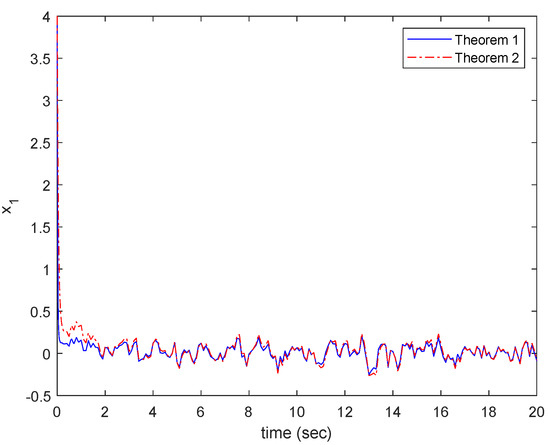
Figure 2.
Response of x1.
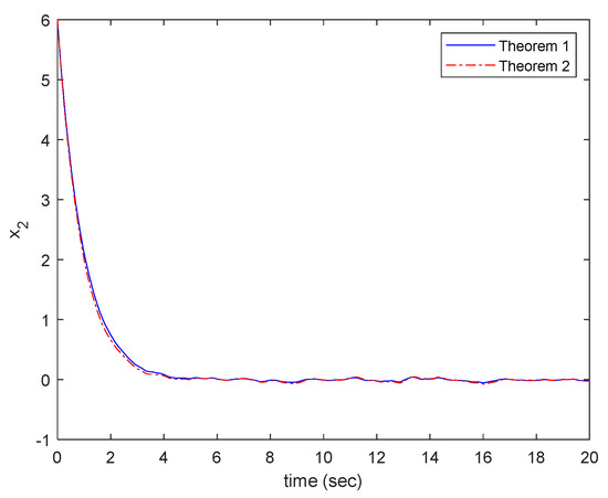
Figure 3.
Response of x2.
Case 2:
In this case, the effectiveness of Theorem 2 is, respectively, verified to design the corresponding PDPF controller, such that the NTV system (40)–(42) is robust stable and passive. Additionally, the required parameters for applying theorems are the same as the ones in Case 1. Besides, the scalars, as and , are set. By using Theorem 1 in the PDPF model (43) and (44), the feasible solutions can be found via SOSTOOLS to build the following PDPF controller.
where , , , , , , , , , , , , , , and .
Besides, the following PDPF controller is designed by the corresponding feasible solutions satisfying Theorem 2.
where , , , , , , , , , , , , , , and .
With the designed PDPF controllers and , the responses of (40)–(42) are, respectively, sated in Figure 4 and Figure 5 with the same initial condition as . Additionally, the external disturbance is chosen as zero mean white noise with unit variance. Besides, the responses of the PDPF controllers and are also provided in Figure 6 and Figure 7.

Figure 4.
Response of x1.
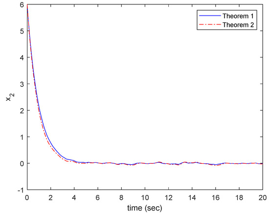
Figure 5.
Response of x2.
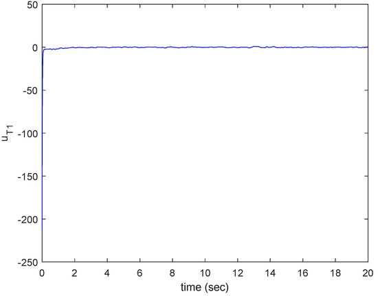
Figure 6.
Response of uT1.
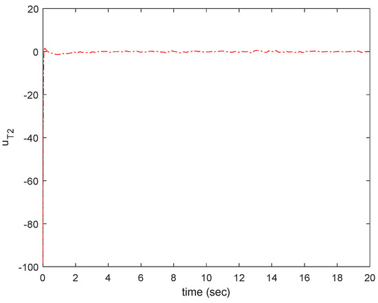
Figure 7.
Response of uT2.
Referring to the figures, although the vibration caused by external disturbance is not eliminated, the responses of (40)–(42), driven by the controllers, are kept around zero. Thus, the robust stability of the PDPF model (40)–(42) is achieved by the designed controller. The following values can be obtained by introducing the simulation results into the passivity inequality in Definition 2.
Additionally,
The value in (47) is obtained by the responses of (40)–(42) driven by (45). Besides, the value in (48) is obtained by the responses of (40)–(42) driven by (46). Those values are smaller than one that satisfies the inequality in Definition 2. Thus, both controller (45) and controller (46), respectively, designed by Theorem 1 and Theorem 2, achieve the passivity of the system (43) and (44) under external disturbance. From Figure 4, it easily finds that the vibration in (40)–(42) driven by (45) is smaller than one driven by (46). Referring to [29], a small value satisfying the passive inequality is better in constraining the effect of external disturbance on the system. Based on (47) and (48), the value obtained by the controller (45) designed by Theorem 1 is smaller than the one designed by Theorem 2. It further demonstrates that the control performance provided by Theorem 1 is better than the one provided by Theorem 2. That means Theorem 1 provides better controller performance than Theorem 2 because the information of system is not considered by the conditions in Theorem 1. Although Theorem 1 provides conservative solutions in searching feasible solutions, the PDPF controller designed by Theorem 1 possesses better performance in stabilizing the NTV system (40)–(42).
- B.
- Ship fin stabilizing system
The following ship fin stabilizing system, with external disturbance, is introduced to show the applicability of the proposed controller designed method.
Through the modelling approaches, system (49)–(51) can be represented by the following PDPF model.
where , , , , , , , , , , , , , , and . is the membership function and shown in the Figure 8.
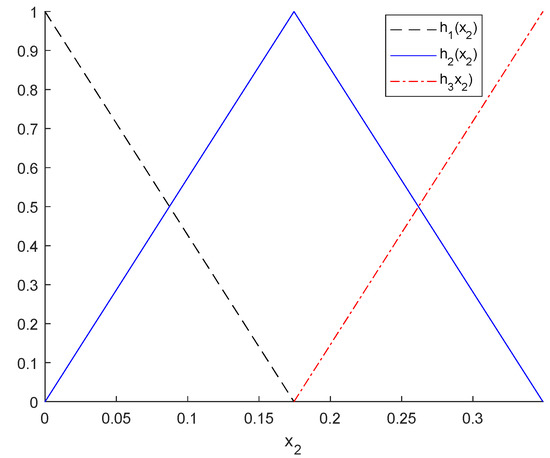
Figure 8.
Membership functions of system (40).
To show the applicability, the method in [32] is introduced to compare with the proposed method. Since the upper and lower bound of time-varying parameter are opposite signs, only Theorem 1 can be applied to system (49)–(51). To apply Theorem 1, the required parameters are given as S1 = I, , , , , , and , in which . In this simulation, is chosen for simplifying the calculation. By using Theorem 1 to PDPF model (52) and (53), feasible solutions can be found via SOSTOOLS to build the following PDPF controller.
where , , , , , , , , , , , , , , , , , , and .
Besides, the control gains in [32] are utilized to build a controller in the comparison. After designing the PDPF controller , the responses in (49)–(52) are, respectively, sated in Figure 9 and Figure 10 with the same initial condition as . The external disturbance is chosen as zero mean white noise with unit variance.
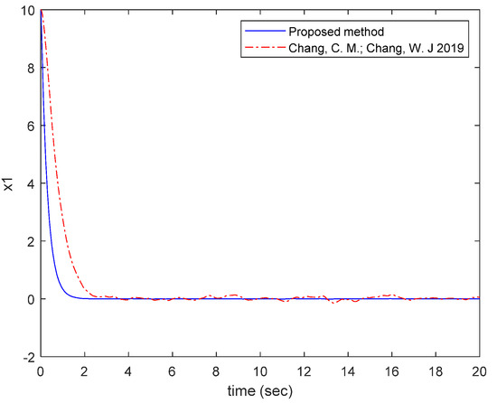
Figure 9.
Response of x1 [32].
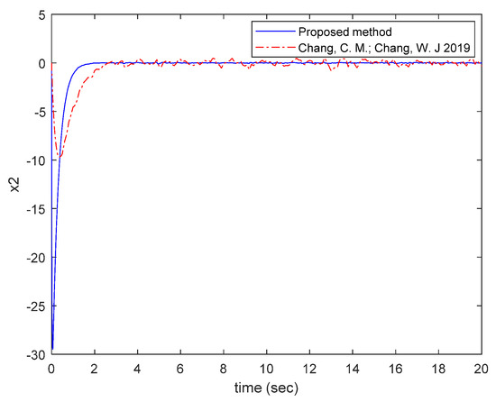
Figure 10.
Response of x2 [32].
As Figure 9 and Figure 10 show, although system (49)–(52) is affected by external disturbance, the responses driven by two controllers are kept around the zero. However, the responses driven by are better than the controller obtained from [32]. The fuzzy rules of the proposed method are less than the method in [32] because the proposed method is based on the polynomial description. Namely, the proposed method provides better performance with less fuzzy rules than the method in [32].
5. Conclusions
In this paper, the stabilization and constraining disturbance effect issue for NTV systems represented by PDPF model was studied via designing the PDPF controller. Based on the modelling approach, the time-varying parameters were interpreted via the convex combination for general description. Owing to the convex combination, the positive definition of the parameter-dependent polynomial Lyapunov function can be held. Moreover, the limitation as an opposite sign of time-varying function can also be ignored for the constraint of time-varying parameters. Furthermore, passivity was considered to constrain the effect of external disturbance on the system. To discuss the issue, some sufficient conditions were derived into SOS form to find the parameter-dependent polynomial gains. Besides, the other stability criterion was proposed by introducing some slack variables to further increase relaxation when discussing the issue. Both proposed criteria can be used to design the corresponding PDPF controller, such that the NTV system achieves stability and attenuation performance. Although Theorem 2 provides a relaxed solution, the limitation as the opposite sign must be avoided. On the other hand, no limitation in system description is avoided by using Theorem 1. Therefore, one should pay attention in applying Theorem 2 for analyzing and synthesizing NTV systems. At last, the two simulation results were provided to show the effectiveness and application of this paper. With the simulation results, the stability and passivity of the systems can be achieved by the design PDPF controller. In general, the proposed method can also be applied to common NTV by setting the degree of the polynomials. Additionally, the passivity performance can be reduced as a suitable performance by setting , and . Besides, the differential of the polynomial Lyapunov function is still an interesting problem for the convex problem. Thus, the novel idea dealing with the derivative of polynomial Lyapunov function will be concerned in the future.
Author Contributions
Supervision, C.-C.K.; investigation, C.-C.S. and S.-H.J.; writing—original draft, S.-H.J.; formal analysis, W.-J.C. All authors have read and agreed to the published version of the manuscript.
Funding
This research received no external funding.
Data Availability Statement
All relevant data displayed in publication.
Conflicts of Interest
The authors declare no conflict of interest.
References
- Nesterov, Y.; Nemirovskii, A. Interior Point Polynomial Algorithms in Convex Programming; Society for Industrial and Applied Mathematics: Philadelphia, PA, USA, 1994. [Google Scholar]
- Prajna, S.; Papachristodoulou, A.; Wu, F. Nonlinear Control Synthesis by Sum of Squares Optimization: A Lyapunov-based Approach. Proc. Asian Control Conf. 2004, 1, 157–165. [Google Scholar]
- Zuluaga, L.F.; Vera, J.; Pena, J. LMI Approximations for Cones of Positive Semidefinite Forms. SIAM J. Optim. 2006, 16, 1076–1091. [Google Scholar] [CrossRef]
- Kavikumar, R.; Sakthivel, R.; Kwon, O.M.; Kaviarasan, B. Faulty Actuator-Based Control Synthesis for Interval Type-2 Fuzzy Systems via Memory State Feedback Approach. Int. J. Syst. Sci. 2020, 51, 2958–2981. [Google Scholar] [CrossRef]
- Kavikumar, R.; Sakthivel, R.; Liu, Y. Design of -based Sampled-Data Control for Fuzzy Markov Jump Systems with Stochastic Sampling. Nonlinear Anal. Hybrid Syst. 2021, 41, 101041. [Google Scholar] [CrossRef]
- Vandenberghe, L.; Boyd, S. Applications of Semidefinite Programming. Appl. Numer. Math. 1999, 29, 1283–1299. [Google Scholar] [CrossRef]
- Ebenbauer, C.; Allgöwer, F. Analysis and Design of Polynomial Control Systems using Dissipation Inequalities and Sum of Squares. Comput. Chem. Eng. 2006, 30, 1590–1602. [Google Scholar] [CrossRef]
- Waki, H.; Nakata, M.; Muramatsu, M. Strange Behaviors of Interior-Point Methods for Solving Semidefinite Programming Problems in Polynomial Optimization. Comput. Optim. Appl. 2012, 53, 823–844. [Google Scholar] [CrossRef]
- Tanaka, K.; Komatsu, T.; Ohtake, H.; Wang, H.O. Micro Helicopter Control: LMI Approach vs SOS Approach. Proc. IEEE Int. Conf. Fuzzy Syst. 2008, 347–353. [Google Scholar] [CrossRef]
- Tanaka, K.; Yoshida, H.; Ohtake, H.; Wang, H.O. A Sum of Squares Approach to Modeling and Control of Nonlinear Dynamical Systems with Polynomial Fuzzy Systems. IEEE Trans. Fuzzy Syst. 2009, 17, 911–922. [Google Scholar] [CrossRef]
- Lam, H.K. Polynomial fuzzy model-based control systems. In Stability Analysis and Control Synthesis Using Membership Function-Dependent Techniques; Springer: Berlin/Heidelberg, Germany, 2016. [Google Scholar]
- Narimani, M.; Lam, H.K. SOS-Based Stability Analysis of Polynomial Fuzzy-Model-Based Control Systems Via Polynomial Membership Functions. IEEE Trans. Fuzzy Syst. 2010, 18, 862–871. [Google Scholar] [CrossRef]
- Chen, Y.J.; Tanaka, K.; Tanaka, M.; Tsai, S.H. A Novel Path-Following-Method-Based Polynomial Fuzzy Control Design. IEEE Trans. Cybern. 2019, 51, 2993–3003. [Google Scholar] [CrossRef]
- Furqon, R.; Chen, Y.J.; Tanaka, M.; Tanaka, K.; Wang, H.O. An SOS-based Control Lyapunov Function Design for Polynomial Fuzzy Control of Nonlinear Systems. IEEE Trans. Fuzzy Syst. 2016, 25, 775–787. [Google Scholar] [CrossRef]
- Tanaka, K.; Ohtake, H.; Wang, H.O. Guaranteed Cost Control of Polynomial Fuzzy Systems via a Sum of Squares Approach. IEEE Trans. Syst. Man Cybern. Part B Cybern. 2008, 39, 561–567. [Google Scholar] [CrossRef]
- Lam, H.K.; Tsai, S.H. Stability Analysis of Polynomial-Fuzzy-Model-Based Control Systems with Mismatched Premise Membership Functions. IEEE Trans. Fuzzy Syst. 2013, 22, 223–229. [Google Scholar] [CrossRef]
- Zhang, H.; Wang, Y.; Wang, Y.; Zhang, J. A Novel Sliding Mode Control for a Class of Stochastic Polynomial Fuzzy Systems Based on SOS Method. IEEE Trans. Cybern. 2019, 50, 1037–1046. [Google Scholar] [CrossRef]
- Xiao, B.; Lam, H.K.; Zhong, Z.; Wen, S. Membership-Function-Dependent Stabilization of Event-Triggered Interval Type-2 Polynomial Fuzzy-Model-Based Networked Control Systems. IEEE Trans. Fuzzy Syst. 2019, 28, 3171–3180. [Google Scholar] [CrossRef]
- Lo, J.C.; Liu, J.W. Polynomial static output feedback control via homogeneous Lyapunov functions. Int. J. Robust Nonlinear Control 2019, 29, 1639–1659. [Google Scholar] [CrossRef]
- Han, H. An Observer-Based Controller for a Class of Polynomial Fuzzy Systems with Disturbance. IEEJ Trans. Electr. Electron. Eng. 2016, 11, 236–242. [Google Scholar] [CrossRef]
- Lee, L.H.; Poolla, K. Identification of Linear Parameter-Varying Systems Using Nonlinear Programming. ASME J. Dyn. Syst. Meas. Control 1999, 121, 71–78. [Google Scholar] [CrossRef]
- Rugh, W.J.; Shamma, J.S. Research on Gain Scheduling. Automatica 2000, 36, 1401–1425. [Google Scholar] [CrossRef]
- Leith, D.J.; Leithead, W.E. Survey of Gain Scheduling Analysis and Design. Int. J. Control 2000, 73, 1001–1025. [Google Scholar] [CrossRef]
- Fu, R.; Sun, H.; Zeng, J. Exponential Stabilisation of Nonlinear Parameter-varying Systems with Applications to Conversion Flight Control of a Tilt Rotor Aircraft. Int. J. Control 2019, 92, 2473–2483. [Google Scholar] [CrossRef]
- Tang, Y.; Li, Y.; Cui, T.; Zheng, Y. Off-equilibrium Linearisation-based Nonlinear Control of Turbojet Enginese with Sum of Squares Programming. Aeronaut. J. 2020, 124, 1879–1895. [Google Scholar] [CrossRef]
- Hooshmandi, K.; Bayat, F.; Jahed-Motlagh, M.R.; Jalali, A.A. Polynomial LPV Approach to Robust Control of Nonlinear Sampled-data Systems. Int. J. Control 2020, 93, 2145–2160. [Google Scholar] [CrossRef]
- Lam, H.K.; Seneviratne, L.D.; Ban, X. Fuzzy Control of Nonlinear Systems Using Parameter-dependent Polynomial Fuzzy Model. IET Control Theory Appl. 2012, 6, 1645–1653. [Google Scholar] [CrossRef]
- Ku, C.C.; Wu, C.I. Gain-Scheduled Control for Linear Parameter Varying Stochastic Systems. ASME J. Dyn. Syst. Meas. Control 2015, 137, 111012. [Google Scholar] [CrossRef]
- Lozano, R.; Brogliato, B.; Egeland, O.; Maschke, B. Dissipative Systems Analysis and Control Theory and Application; Springer Science & Business Media: London, UK, 2000. [Google Scholar]
- Papachristodoulou, A.; Prajna, S. A Tutorial on Sum of Squares Techniques for Systems Analysis. Proc. Am. Control Conf. 2005, 49, 2686–2700. [Google Scholar]
- Parrilo, P.A. Structured Semidefinite Programs and Semialgebraic Geometry Methods in Robustness and Optimization. Ph.D. Thesis, California Institute of Technology, Pasadena, CA, USA, 2000. [Google Scholar]
- Chang, C.M.; Chang, W.J. Robust Fuzzy Control with Transient and Steady-State Performance Constraints for Ship Fin Stabilizing Systems. Int. J. Fuzzy Syst. 2019, 21, 518–531. [Google Scholar] [CrossRef]


Disclaimer/Publisher’s Note: The statements, opinions and data contained in all publications are solely those of the individual author(s) and contributor(s) and not of MDPI and/or the editor(s). MDPI and/or the editor(s) disclaim responsibility for any injury to people or property resulting from any ideas, methods, instructions or products referred to in the content. |
© 2023 by the authors. Licensee MDPI, Basel, Switzerland. This article is an open access article distributed under the terms and conditions of the Creative Commons Attribution (CC BY) license (https://creativecommons.org/licenses/by/4.0/).