Transfer Learning-Based Coupling of Smoothed Finite Element Method and Physics-Informed Neural Network for Solving Elastoplastic Inverse Problems

Abstract

In practical engineering applications, there is a high demand for inverting parameters for various materials, and obtaining monitoring data can be costly. Traditional inverse methods often involve tedious computational processes, require significant computational effort, and exhibit slow convergence speeds. The recently proposed Physics-Informed Neural Network (PINN) has shown great potential in solving inverse problems. Therefore, in this paper, we propose a transfer learning-based coupling of the Smoothed Finite Element Method (S-FEM) and PINN methods for the inversion of parameters in elastic-plasticity problems. The aim is to improve the accuracy and efficiency of parameter inversion for different elastic-plastic materials with limited data. High-quality small datasets were synthesized using S-FEM and subsequently combined with PINN for pre-training purposes. The parameters of the pre-trained model were saved and used as the initial state for the PINN model in the inversion of new material parameters. The inversion performance of the coupling of S-FEM and PINN is compared with the coupling of the conventional Finite Element Method (FEM) and PINN on a small data set. Additionally, we compared the efficiency and accuracy of both the transfer learning-based and non-transfer learning-based methods of the coupling of S-FEM and PINN in the inversion of different material parameters. The results show that: (1) our method performs well on small datasets, with an inversion error of essentially less than 2%; (2) our approach outperforms the coupling of conventional FEM and PINN in terms of both computational accuracy and computational efficiency; and (3) our approach is at least twice as efficient as the coupling of S-FEM and PINN without transfer learning, while still maintaining accuracy. Our method is well-suited for the inversion of different material parameters using only small datasets. The use of transfer learning greatly improves computational efficiency, making our method an efficient and accurate solution for reducing computational cost and complexity in practical engineering applications.

1. Introduction

The inverse problem of determining the cause, condition, or input from the effect, performance, or output has been proposed in many fields of scientific research and is commonly referred to as a “mathematical-physical inverse problem” [1]. The importance and necessity of studying inverse problems have been recognized, driven by the needs of natural science and engineering applications. In recent decades, inverse problems have found extensive applications in fields such as geophysics [2,3,4], resource exploration [5,6], ocean engineering [7], mechanics [8,9,10], acoustics [11,12], and others.

Traditional mechanical inverse analysis methods usually employ a combination of numerical methods and optimization algorithms. An optimization algorithm is a mathematical method that minimizes or maximizes an objective function by adjusting model parameters or design variables [13]. In mechanical inverse analysis, optimization algorithms are used to adjust model parameters or design variables to minimize the error between simulation results and actual observed or desired results. Traditional mechanical inverse analysis methods typically employ iterative optimization algorithms to incrementally enhance the model, with commonly used algorithms including gradient descent [14], genetic algorithms [15], and particle swarm optimization [16]. However, these conventional optimization algorithms have limitations such as the tendency to converge to local optima and slow convergence speeds. Consequently, numerous novel optimization algorithms have emerged to address these drawbacks. Examples include the Arithmetic Optimization Algorithm [17], the IbI Logic Algorithm [18], and the modified Sooty Tern Optimization Algorithm [13].

Many researchers have effectively utilized numerical methods and optimization algorithms for the identification of mechanical parameters in elastoplastic materials. For example, De-Carvalho et al. [14] employed two optimization algorithms, namely, the gradient-based Levenberg–Marquardt algorithm and the real search space evolution algorithm, to perform inverse analysis on the constitutive parameters of three different models: the elastic-plastic hardening model, the hyperelastic model, and the elastic-viscoplastic model. The objective was to minimize the disparity between the physical experimental results and the numerical simulation results [14]. Furthermore, a significant number of studies have utilized probability-based parameter estimation methods for mechanical parameter identification. For instance, Khodadadian et al. [19] developed a Bayesian parameter estimation framework to identify the uncertain parameters associated with the phase field fracture problem. Reliable results are obtained by their proposed Bayesian inversion method, even when relatively coarse grids are employed instead of real data [19]. Similarly, Noii et al. [20] applied Bayesian inversion techniques to identify mechanical parameters in various scenarios, including linear elasticity, elastoplasticity, and fracture problems of different materials. They extensively investigated the complex coupled multi-field marginal value problem and shared the open source code of their Bayesian inversion method [20].

However, traditional mechanical inverse analysis methods suffer from cumbersome inversion processes, large computations, and slow convergence efficiencies. The rapid development of artificial intelligence techniques, particularly the impressive capabilities of deep learning in handling high-dimensional complex structural data, have made them powerful tools for solving both forward and inverse problems in mechanics [9,21,22,23,24]. For instance, Liu et al. [21,22] proposed a two-way neural network for solving both forward and inverse problems in mechanics, which they combined with nonlinear finite elements to accurately identify the constitutive parameters of hyperelastic materials. Potrzeszcz-Sut et al. [9] utilized a backpropagation neural network in conjunction with indentation test data to efficiently determine the elastic-plastic material parameters described by Ramberg–Osgood’s law. Pichler et al. [24] employed artificial neural networks to approximate finite element analysis and combined them with genetic algorithms to determine optimal parameter estimates for unknown parameter identification. In a similar vein, Liu et al. [25] introduced a surrogate model based on orthogonal decomposition and artificial neural networks. They further integrated this surrogate model with Bayesian theory to achieve the efficient inversion of geotechnical parameters.

Despite the great strides made in deep learning, it cannot be overlooked that its current achievements rely heavily on large, high-quality datasets. However, in practical engineering problems, obtaining a significant amount of high-quality data is often challenging due to measurement difficulties, high costs, and measurement errors. As a result, the accuracy of the computational results may be low or difficult to solve directly using purely data-driven deep learning methods.

In the latest research work, the physics-informed deep learning method proposed by Professor Karniadakis constructs interpretable neural network models by incorporating relevant physical laws or constraints [26]. Physics-informed deep learning guarantees the generalization and validity of the model, even when there is a small amount of data or when noise observation bias, or other such factors are present. 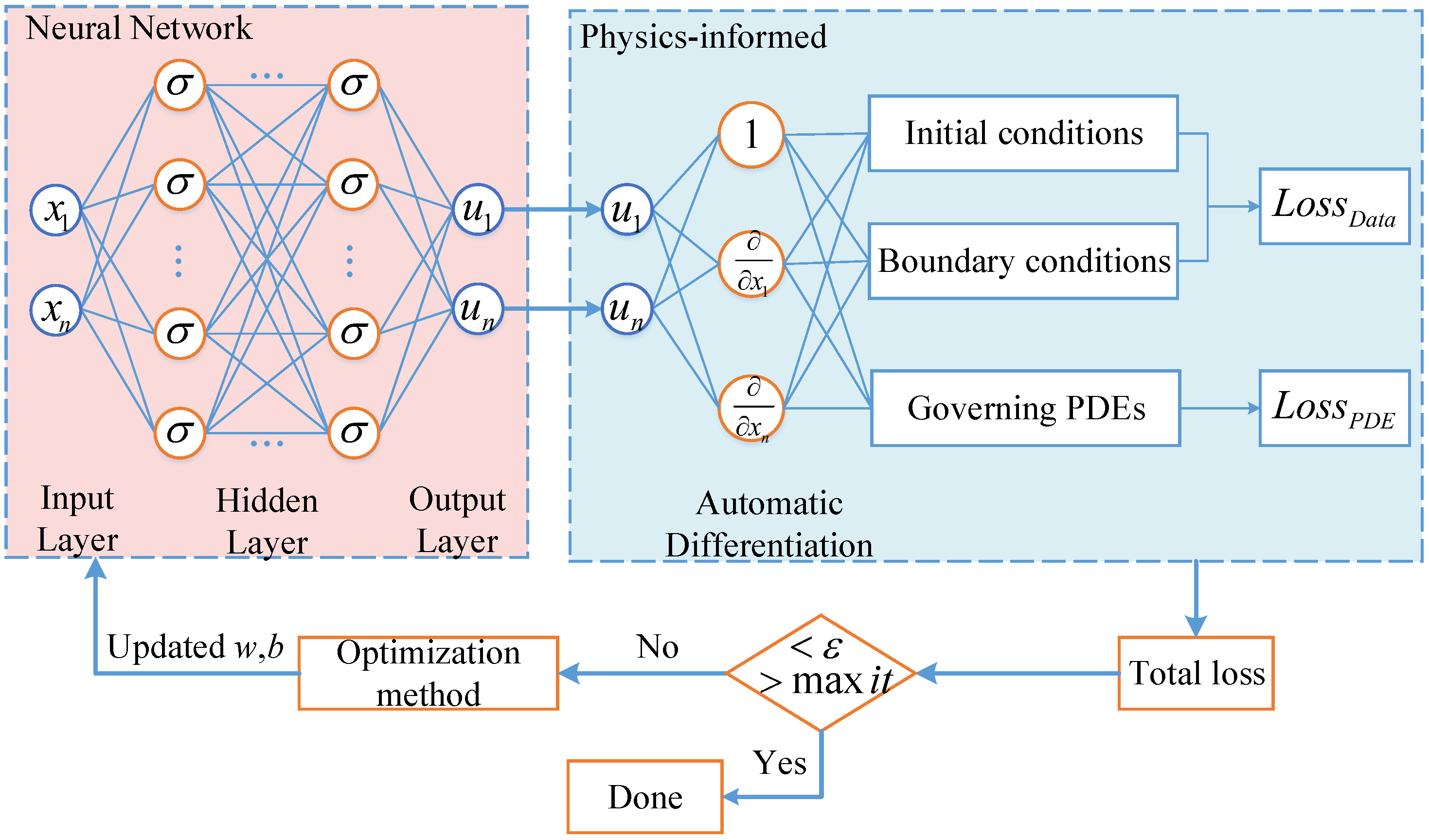This approach enables the model predictions to comply with objective physical constraints [26], ensuring their accuracy and reliability. A typical example of this is the Physics-Informed Neural Network (PINN), which shows great promise in solving both the forward and inverse problems of partial differential equations (PDEs). This is due to its ability to integrate data and PDEs [27,28,29], making it a powerful tool for researchers in the field. PINNs have proven to be effective in solving many inverse problems of PDEs due to their ease of implementation. This is because the code used for solving the forward problem can be applied to the solution of the inverse problem with minimal modifications [8,30,31,32].

For example, Fallah et al. [30] utilized PINN to invert the natural frequency of TDFG porous beams on an elastic foundation. They then used this information to solve for the bending and free vibrations of TDFG porous beams using PINN. Depina et al. [31] applied PINNs to the inverse problem of unsaturated groundwater flow. Their research demonstrated that PINNs are capable of accurately identifying the van Genuchten constitutive parameters. Xu et al. [32] improved the training efficiency and accuracy of neural networks for linear elastic and hyperelastic inverse problems by incorporating uncertainty-weighted multi-task learning methods and transfer learning strategies based on PINN. Lu et al. [8] employed physics-informed deep learning to improve the accuracy and efficiency of the inversion process for the mechanical properties of elastic-plastic materials.

Due to the challenges associated with acquiring real measurement data, researchers often resort to numerical methods to synthesize data used to train PINNs when tackling inverse problems involving PDEs. These trained PINNs are subsequently applied to real-world engineering problems where only limited measurement data are available [8,32]. The computational errors arising from numerical methods can be regarded as measurement errors, and PINNs demonstrate robustness in handling such errors. The Finite Element Method (FEM) is commonly employed as the primary numerical method. However, it has certain limitations, such as its high dependency on mesh quality, its inability to handle mesh distortion, and its susceptibility to volume locking issues [33]. To address these problems, the Smoothed Finite Element Method (S-FEM) has been developed. S-FEM is an extension of the FEM that incorporates the smoothing strain technique, enabling it to handle mesh distortion effectively. Moreover, S-FEM offers improved computational accuracy compared to FEM [33,34,35]. Due to the geometric complexity and irregularity of practical engineering problems, achieving high computational accuracy with quadrilateral cells in the discretization process becomes challenging. In contrast, triangular cells in the S-FEM offer better accuracy when properly adapted to the geometry. Therefore, the use of triangular cells reduces computational complexity while ensuring a better adaptation to real engineering problems [36].

In practical engineering applications, there is a growing need to invert various material parameters. However, traditional machine learning is typically designed for specific tasks, requiring reconstruction of the model after changing the dataset. This can result in a significant increase in computational cost. Transfer learning involves utilizing knowledge from a previously trained model for a new task [37]. For instance, the weights and biases from a pre-trained neural network can be used as initial values for a neural network trained on a similar problem. By avoiding random initialization of the neural network, the training process can converge more quickly.

The combination of transfer learning with PINN for parameter inversion has received relatively little attention in research. Haghighat et al. [38] proposed a PINN framework for solving inverse problems in solid mechanics, but only briefly mentioned its potential for transfer learning without conducting significant analysis or research on the topic. Xu et al. [32] proposed a transfer learning-based PINN method for inverting different loading systems of linear-elastic and hyperelastic structures. However, due to the characteristics of transfer learning, the method presented in [32] still requires a significant amount of data in the pre-training phase.

In this paper, we propose a transfer learning-based coupling of S-FEM and PINN approach to invert different material parameters, with the goal of improving the accuracy and efficiency of the inversion process. The proposed approach involves utilizing S-FEM to generate a small dataset of high quality, which is then combined with PINN for pre-training purposes. The resulting pre-trained model parameters are saved and utilized as the initial state for the PINN model when inverting the material parameters of a new dataset. To assess the accuracy and efficiency of the proposed method during the pre-training phase, validation will be conducted using an elastic-plastic material parameter inversion problem. Subsequently, the inversion of various material parameters, encompassing linear elasticity and elastoplasticity, will be performed by employing the coupling of S-FEM and PINN, both with and without transfer learning.

The contributions of this paper can be summarized as follows:

(1)

A transfer learning-based coupling of the S-FEM and PINN methods for the inversion of different material parameters is proposed.

(2)

The proposed approach improves the convergence efficiency of the inversion by at least a factor of two over the method without transfer learning and also provides a degree of improvement in the accuracy of the inversion.

(3)

The proposed method requires only a small amount of data in the pre-training phase of the model to achieve high accuracy.

This paper is organized as follows. The backgrounds of the S-FEM, PINN, and elastic-plastic problems are presented in Section 2. The PDEs involved in the elastoplastic inversion problem and the specific implementation of our proposed approach are illustrated in Section 3. The results of our proposed method to invert different material parameters are presented in Section 4. The advantages and disadvantages of our proposed method and the future research work are discussed in Section 5. Finally, a summary of the paper is presented.

2. Background

In this section, the basic idea of S-FEM is introduced, highlighting the distinctions between S-FEM and FEM. Additionally, a concise overview of the research progress and fundamental principles of PINN is provided. Finally, a brief introduction is given to the elastic-plasticity problem along with its engineering application background.

2.1. Smoothed Finite Element Method (S-FEM)

The FEM is one of the most widely used numerical methods in solid mechanics. It is a very effective tool for solving complex differential equations or PDEs, especially nonlinear systems of PDEs [39]. Although the FEM is used extensively in engineering science, the demand for greater accuracy and stability in its results has led to a greater focus on the limitations of the traditional FEM. The displacement finite element theory is widely used in commercial finite element software. However, the stiffness matrix of the system obtained based on the displacement finite element method is stiff, which can result in a small displacement solution and a large intrinsic frequency solution [33]. During the solution process, conversions and mappings of local and global coordinate systems occur. Therefore, the problem domain needs to be discretized with only regular grids and not distorted grids to ensure high solution accuracy, as distorted grids can significantly impact the accuracy of the solution [35].

To address the limitations of the FEM, several numerical methods have been proposed, including the S-FEM [40,41,42,43]. The S-FEM, proposed by Liu G.R., combines the benefits of the FEM and the mesh-free method. This method can address issues such as mesh distortion and volume locking problems while also improving computational accuracy [35]. The fundamental principle of S-FEM is to divide the integration region into smoothing subdomains based on the mesh of finite elements. These subdomains are required to follow the rules of being interconnected and not overlapping [35]. S-FEM can be categorized into several types depending on the method of division. These include cell-based S-FEM (CS-FEM) [44,45], node-based S-FEM (NS-FEM) [46], edge-based S-FEM (ES-FEM) [36], face-based S-FEM (FS-FEM) [47], and hybrid S-FEM (HS-FEM) [48]. S-FEM utilizes the finite element background mesh to construct the shape function and perform smoothing strain computation in the smoothing domain constructed on the background mesh. It also uses a gradient-smoothing technique that transforms the area integral into a boundary integral, thereby significantly improving computational accuracy, enhancing the adaptability of low-order cells to mesh distortions, and effectively softening the system stiffness [35]. In contrast to FEM, S-FEM uses linear point interpolation to represent the shape function. Therefore, coordinate transformation is not required, and there is no need to calculate the derivatives of the shape function [35]. Due to the absence of the mapping of shape functions, S-FEM is stable when dealing with irregular meshes. Moreover, S-FEM has high convergence and accuracy because of the softened stiffness matrix.

2.2. Physics-Informed Neural Network (PINN)

PINNs leverage prior knowledge by integrating observational data and mathematical models to efficiently solve both forward and inverse problems of PDEs. Currently, PINNs have demonstrated remarkable success in various mechanics fields, including material mechanics [38], fluid mechanics [49], fracture mechanics [50], and thermodynamics [51]. Several PINN variants have emerged to address different problems, including conservation PINNs (cPINNs) [52], variational PINNs (vPINNs) [53], fractional-order PINNs (fPINNs) [54], and others. Additionally, many researchers have optimized and improved the training process, activation functions, and generalization error of PINNs [55,56]. Furthermore, open-source PINN library packages, such as SciANN [57], DeepXDE [58], and SimNet [59], make it easier to apply PINNs to solve specific problems.

The basic framework of PINN consists of two components: a neural network approximation function and physical information constraints, as illustrated in Figure 1. The input data are approximated using a fully connected neural network to generate predicted values. An automatic differentiation algorithm is used to obtain the residuals of the physical information from the predicted values. These residuals are then incorporated into the loss function as a regular term constraint. The neural network’s weight parameters and deviation vectors are connected and trained using the gradient descent algorithm until the residuals reach the convergence condition, at which point training stops. This process ultimately leads to the solution of the model parameters and the prediction of the results.

As shown in Figure 1, $x_1$ and $x_n$ are the inputs of the neural network, $\sigma$ is the activation function, and $u_1$ and $u_n$ are the outputs of the neural network. The results of the automatic differentiation computation using the neural network are denoted as 1, $\frac{\partial }{\partial x_1}$, and $\frac{\partial }{\partial x_n}$. $Los{s}_{Data}$ represents the data-driven partial residuals, and $Los{s}_{PDE}$ represents the physically constrained partial residuals. $\epsilon$ is the threshold of the loss function, $maxit$ is the maximum number of training steps, and w and b are the weights and biases of the neural network, respectively.

Traditional physical models are used to solve PDEs by giving the initial state, boundary states, and physical parameters at any point. When analytical solutions are not available, numerical methods such as FEM and Finite Difference Method (FDM) are often employed to solve the PDEs. The PINN is a deep neural network-based approach that incorporates physical information into neural networks to approximate the solutions of PDEs. In this method, the model residuals comprise two components: the residuals of the data and the residuals of the physical information, i.e., $Loss=Los{s}_{Data}+Los{s}_{PDE}$.

$$Los{s}_{Data}=\frac{1}{N_{Data}}\sum _{i=1}^{N_{Data}}{\left|u^N(x_i,y_i)-u_i\right|}^2$$

(1)

Equation (1) represents the data-driven partial residuals, where ${\left\{u^N(x_i,y_i)\right\}}_{i=1}^{N_{Data}}$ denotes the result obtained from the neural network prediction; ${\left\{u_i\right\}}_{i=1}^{N_{Data}}$ is the known data, including initial and boundary conditions as well as the measured and synthetic data; and $N_{Data}$ is the number of known data points.

$$Los{s}_{PDE}=\frac{1}{N_{PDE}}\sum _{i=1}^{N_{PDE}}{\left|r(x_i,y_i)\right|}^2$$

(2)

Equation (2) represents the physically constrained partial residuals, where ${\left\{r(x_i,y_i)\right\}}_{i=1}^{N_{PDE}}$ is the PDE’s residual and $N_{PDE}$ is the number of configuration points of the PINN.

2.3. Elastoplastic Problems

Elastoplastic mechanics is an important branch of deformable solid mechanics, which is the study of the stress, strain, and displacement of deformable materials and their distribution laws when subjected to external loads, temperature changes, and other factors [60,61]. Most objects generally go through three stages from stress to destruction: elasticity, plasticity, and destruction. The solution of elastic-plastic mechanics problems is crucial in many fields of research, such as civil engineering [62], mechanical engineering [63], aerospace engineering [64], and materials engineering [65].

The basic equations of elastoplastic mechanics need to be established in terms of their geometry, kinematics, and physics [60,61]. Firstly, since elastoplastic mechanics assumes that the object is continuous, all adjacent small units are interconnected during deformation, and the coordination conditions of deformation can be obtained by studying the relationship between displacement and strain [60,61]. The mathematical expressions reflecting the continuous law of deformation are the geometric equations and displacement boundary conditions. Secondly, in the elastic-plastic problem, the object should not only be in equilibrium as a whole but also locally in equilibrium, and the mathematical equations reflecting this law are equilibrium differential equations and load boundary conditions [60,61]. These two types of equations are independent of the mechanical properties of the material and are universal. In physics, it is necessary to establish the relationship between stress and strain or stress and strain increments, and this relationship is called the constitutive relationship. The constitutive relationship describes the mechanical properties of a material in different environments, and the study of the constitutive relationship is crucial in elastoplastic mechanics [60,61].

When tackling an elastoplastic statics problem, several essential elements need to be provided to determine the stresses, strains, and displacements of the object. These include the shape of the object, constitutive relationships, and the physical-mechanical parameters for each component of the object’s material, as well as the load and displacement boundary conditions to which the object is subjected [60,61]. In engineering problems, determining the constitutive parameters, physical-mechanical parameters, and boundary conditions of materials can often prove challenging [66,67]. The concept of inverse problem solving offers a means to determine these parameters. Through the observation of strain or displacement data from the structure, the inverse analysis method in elastic-plastic mechanics can be utilized to infer crucial information such as the constitutive parameters, physical-mechanical parameters, and boundary conditions of the material [66,67].

3. Methods

In this section, the relevant PDEs associated with the elastoplastic mechanic problem are initially presented, highlighting the parameters that necessitate inversion. Subsequently, the implementation process of our proposed approach, which couples S-FEM and PINN based on transfer learning, is described.

3.1. Governing Equations and Parameters

The equations involved in the elastic-plastic problem mainly include equilibrium differential equations, geometric equations, and physical equations. Since the equilibrium differential equations and geometric equations are independent of the material properties, these two types of equations for the linear elastic and elastoplastic problems are consistent, see Equations (3)–(11). Equations (3)–(5) are equilibrium differential equations, and Equations (6)–(11) are geometric equations.

$${\sigma }_{xx,x}+{\sigma }_{yx,y}+{\sigma }_{zx,z}+f_x=0$$

(3)

$${\sigma }_{xy,x}+{\sigma }_{yy,y}+{\sigma }_{zy,z}+f_y=0$$

(4)

$${\sigma }_{xz,x}+{\sigma }_{yz,y}+{\sigma }_{zz,z}+f_z=0$$

(5)

where ${\sigma }_{ij,i}$ ($i,j=x,y,z$) represents the partial derivative of the stress tensor and $f_i$ ($i=x,y,z$) represents the volume force.

$${\epsilon }_{xx}=u_{x,x}$$

(6)

$${\epsilon }_{yy}=u_{y,y}$$

(7)

$${\epsilon }_{zz}=u_{z,z}$$

(8)

$${\epsilon }_{xy}=\frac{1}{2}(u_{x,y}+u_{y,x})$$

(9)

$${\epsilon }_{yz}=\frac{1}{2}(u_{y,z}+u_{z,y})$$

(10)

$${\epsilon }_{zx}=\frac{1}{2}(u_{z,x}+u_{x,z})$$

(11)

where ${\epsilon }_{ij}$ ($i,j=x,y,z$) represents the strain tensor and $u_{i,j}$ ($i,j=x,y,z$) represents the partial derivative of the displacement. ${\sigma }_m=\left({\sigma }_{xx}+{\sigma }_{yy}+{\sigma }_{zz}\right)/3$ is the mean stress and ${\epsilon }_m=\left({\epsilon }_{xx}+{\epsilon }_{yy}+{\epsilon }_{zz}\right)/3$ is the mean strain

For the linear elastic plane strain problem, where ${\epsilon }_{zz}={\epsilon }_{yz}={\epsilon }_{xz}=0$, the physical equations are Equations (12)–(14).

$$(\lambda +2\mu ){\epsilon }_{xx}+\lambda {\epsilon }_{yy}-{\sigma }_{xx}=0$$

(12)

$$(\lambda +2\mu ){\epsilon }_{yy}+\lambda {\epsilon }_{xx}-{\sigma }_{yy}=0$$

(13)

$$2\mu {\epsilon }_{xy}-{\sigma }_{xy}=0$$

(14)

where $\lambda$ and $\mu$ are the Lamé parameters, which have different meanings in various branches of mechanics. In elastoplastic mechanics, $\lambda =\frac{E\nu }{(1+\nu )(1-2\nu )}$ is the Lamé parameter 1 and $\mu =\frac{E}{2(1+\nu )}$ is the Lamé parameter 2, which is also the shear modulus of elasticity in material mechanics, and E and $\nu$ are the Young’s modulus and Poisson’s ratio, respectively. In this paper, $\lambda$ is a known parameter, while $\mu$ is the parameter to be determined through the inversion process.

In the linear elastic plane problem, the PDE residuals and the data residuals can be expressed as Equations (15) and (16).

$$\begin{array}{ccc}\hfill Los{s}_{Data}& =& \frac{1}{N_{Data}}\sum _{i=1}^{N_{Data}}\left({\left|u_x^i-u_x^{i*}\right|}^2+{\left|u_y^i-u_y^{i*}\right|}^2+{\left|{\sigma }_{xx}^i-{\sigma }_{xx}^{i*}\right|}^2\right.\hfill \\ \hfill & +& {\left|{\sigma }_{yy}^i-{\sigma }_{yy}^{i*}\right|}^2\left.+{\left|{\sigma }_{xy}^i-{\sigma }_{xy}^{i*}\right|}^2\right)\hfill \end{array}$$

(15)

$$\begin{array}{ccc}\hfill Los{s}_{PDE}& =& \frac{1}{N_{PDE}}\sum _{i=1}^{N_{PDE}}{\left({\left|{\sigma }_{xx,x}^i+{\sigma }_{xy,y}^i+f_x^{i*}\right|}^2+\left|{\sigma }_{xy,x}^i+{\sigma }_{yy,y}^i+f_y^{i*}\right|\right.}^2\hfill \\ \hfill & +& {\left|(\lambda +2\mu ){\epsilon }_{xx}^i+\lambda {\epsilon }_{yy}^i-{\sigma }_{xx}^i\right|}^2+{\left|(\lambda +2\mu ){\epsilon }_{yy}^i+\lambda {\epsilon }_{xx}^i-{\sigma }_{yy}^i\right|}^2\hfill \\ \hfill & +& \left.{\left|2\mu {\epsilon }_{xy}^i-{\sigma }_{xy}^i\right|}^2\right)\hfill \end{array}$$

(16)

where the physical quantities without an asterisk superscript represent the predicted results obtained from the PINN or are computed based on these predicted results. Moreover, the physical quantities with an asterisk superscript denote the labeled data.

Before establishing the physical equations of the elastic-plastic problem, it is necessary to determine the yield criterion. The yield criterion serves as a condition to discern whether the material is in an elastic or plastic state. In this paper, the von Mises criterion, which is widely applicable to metallic materials, is selected as the yield criterion for the elastoplastic problem (see Equation (17)).

$$\overline{\sigma }=\frac{1}{\sqrt{2}}\sqrt{{\left({\sigma }_{xx}-{\sigma }_{yy}\right)}^2+{\left({\sigma }_{yy}-{\sigma }_{zz}\right)}^2+{\left({\sigma }_{zz}-{\sigma }_{xx}\right)}^2+6\left({\sigma }_{xy}^2+{\sigma }_{yz}^2+{\sigma }_{zx}^2\right)}={\sigma }_s$$

(17)

where $\overline{\sigma }$ is the equivalent stress, ${\sigma }_{ij}$ ($i,j=x,y,z$) represents the stress tensor, and ${\sigma }_s$ is the yield stress of the material, which is the first material parameter to be inverted in an elastoplastic problem. The material is in the elastic state when $\overline{\sigma }<{\sigma }_s$ and in the plastic state when $\overline{\sigma }\ge {\sigma }_s$.

For small elastic-plastic deformation problems, the stress–strain relationship is described by the following equations:

$${\epsilon }_{xx}-{\epsilon }_m=\frac{3}{2}\frac{\overline{\epsilon }}{\overline{\sigma }}({\sigma }_{xx}-{\sigma }_m)$$

(18)

$${\epsilon }_{yy}-{\epsilon }_m=\frac{3}{2}\frac{\overline{\epsilon }}{\overline{\sigma }}({\sigma }_{yy}-{\sigma }_m)$$

(19)

$${\epsilon }_{zz}-{\epsilon }_m=\frac{3}{2}\frac{\overline{\epsilon }}{\overline{\sigma }}({\sigma }_{zz}-{\sigma }_m)$$

(20)

$${\epsilon }_{xy}=\frac{3}{2}\frac{\overline{\epsilon }}{\overline{\sigma }}{\sigma }_{xy}$$

(21)

$${\epsilon }_{yz}=\frac{3}{2}\frac{\overline{\epsilon }}{\overline{\sigma }}{\sigma }_{yz}$$

(22)

$${\epsilon }_{zx}=\frac{3}{2}\frac{\overline{\epsilon }}{\overline{\sigma }}{\sigma }_{zx}$$

(23)

where $\overline{\epsilon }$ is the equivalent strain. According to the power-hardening constitutive relationship, $\overline{\sigma }$ and $\overline{\epsilon }$ can be expressed as Equation (24) in this paper. In the elastic phase, the stress–strain relationship follows Hooke’s law and is linear. However, when the material transitions into the plastic phase, the stress–strain relationship becomes nonlinear, characterized by a power exponent relationship between stress and strain.

$$\overline{\sigma }=\left\{\begin{array}{c}E\overline{\epsilon }\left(0\le \overline{\epsilon }\le {\epsilon }_s\right)\hfill \\ B{\left(\overline{\epsilon }-{\epsilon }_0\right)}^m\left(\overline{\epsilon }\ge {\epsilon }_s\right)\hfill \end{array}\right.$$

(24)

where E is Young’s modulus, the second material parameter to be inverted in the elastoplastic problem. ${\epsilon }_0={\epsilon }_s\left(1-m\right)$, $B=\frac{E{\epsilon }_s}{{\left({\epsilon }_s-{\epsilon }_0\right)}^m}$, m is the power hardening index, and ${\epsilon }_s$ is the equivalent strain corresponding to the yield stress ${\sigma }_s$ of the material.

In the elastoplastic plane stress problem, where ${\sigma }_{zz}={\sigma }_{yz}={\sigma }_{zx}=0$, the PDE residuals and data residuals can be expressed as Equations (25) and (26), respectively. For a three-dimensional (3D) elastic-plastic problem, the PDE residuals and data residuals can be expressed as Equations (27) and (28), respectively.

$$\begin{array}{ccc}\hfill Los{s}_{PDE}& =& \frac{1}{N_{PDE}}\sum _{i=1}^{N_{PDE}}\left({\left|{\sigma }_{xx,x}^i+{\sigma }_{xy,y}^i+f_x^{i*}\right|}^2+{\left|{\sigma }_{xy,y}^i+{\sigma }_{yy,y}^i+f_y^{i*}\right|}^2\right.\hfill \\ \hfill & +& {\left|3\overline{\epsilon }/\left(2\overline{\sigma }\right)({\sigma }_{xx}^i-{\sigma }_m^i)-\left({\epsilon }_{xx}^i\right.-\left.{\epsilon }_m^i\right)\right|}^2\hfill \\ \hfill & +& {\left|3\overline{\epsilon }/\left(2\overline{\sigma }\right)({\sigma }_{yy}^i-{\sigma }_m^i)-\left({\epsilon }_{yy}^i\right.-\left.{\epsilon }_m^i\right)\right|}^2\hfill \\ \hfill & +& {\left|3\overline{\epsilon }/\left(2\overline{\sigma }\right)(-{\sigma }_m^i)-\left({\epsilon }_{zz}^i\right.-\left.{\epsilon }_m^i\right)\right|}^2\hfill \\ \hfill & +& {\left|3\overline{\epsilon }/\left(2\overline{\sigma }\right){\sigma }_{xy}^i-{\epsilon }_{xy}^i\right|}^2\hfill \\ \hfill & +& \left.{\left|({\sigma }_s^i/E)-\left(({\sigma }_s^i/B^{(1/m)})+{\epsilon }_0\right)\right|}^2\right)\hfill \end{array}$$

(25)

$$\begin{array}{ccc}\hfill Los{s}_{Data}& =& \frac{1}{N_{Data}}\sum _{i=1}^{N_{Data}}\left({\left|u_x^i-u_x^{i*}\right|}^2+{\left|u_y^i-u_y^{i*}\right|}^2\right.\hfill \\ \hfill & +& \left.{\left|{\sigma }_{xx}^i-{\sigma }_{xx}^{i*}\right|}^2+{\left|{\sigma }_{yy}^i-{\sigma }_{yy}^{i*}\right|}^2+{\left|{\sigma }_{xy}^i-{\sigma }_{xy}^{i*}\right|}^2\right)\hfill \end{array}$$

(26)

$$\begin{array}{ccc}\hfill Los{s}_{PDE}& =& \frac{1}{N_{PDE}}\sum _{i=1}^{N_{PDE}}\left({\left|{\sigma }_{xx,x}^i+{\sigma }_{xy,y}^i+{\sigma }_{xz,z}^i+f_x^{i*}\right|}^2+{\left|{\sigma }_{xy,y}^i+{\sigma }_{yy,y}^i+{\sigma }_{yz,z}^i+f_y^{i*}\right|}^2\right.\hfill \\ \hfill & +& {\left|{\sigma }_{xz,x}^i+{\sigma }_{yz,y}^i+{\sigma }_{zz,z}^i+f_z^{i*}\right|}^2+{\left|3\overline{\epsilon }/\left(2\overline{\sigma }\right)({\sigma }_{xx}^i-{\sigma }_m^i)-\left({\epsilon }_{xx}^i\right.-\left.{\epsilon }_m^i\right)\right|}^2\hfill \\ \hfill & +& {\left|3\overline{\epsilon }/\left(2\overline{\sigma }\right)({\sigma }_{yy}^i-{\sigma }_m^i)-\left({\epsilon }_{yy}^i\right.-\left.{\epsilon }_m^i\right)\right|}^2+{\left|3\overline{\epsilon }/\left(2\overline{\sigma }\right)({\sigma }_{zz}^i-{\sigma }_m^i)-\left({\epsilon }_{zz}^i\right.-\left.{\epsilon }_m^i\right)\right|}^2\hfill \\ \hfill & +& {\left|3\overline{\epsilon }/\left(2\overline{\sigma }\right){\sigma }_{xy}^i-{\epsilon }_{xy}^i\right|}^2+{\left|3\overline{\epsilon }/\left(2\overline{\sigma }\right){\sigma }_{yz}^i-{\epsilon }_{yz}^i\right|}^2+{\left|3\overline{\epsilon }/\left(2\overline{\sigma }\right){\sigma }_{zx}^i-{\epsilon }_{zx}^i\right|}^2\hfill \\ \hfill & +& \left.{\left|({\sigma }_s^i/E)-\left(({\sigma }_s^i/B^{(1/m)})+{\epsilon }_0\right)\right|}^2\right)\hfill \end{array}$$

(27)

$$\begin{array}{ccc}\hfill Los{s}_{Data}& =& \frac{1}{N_{Data}}\sum _{i=1}^{N_{Data}}\left({\left|u_x^i-u_x^{i*}\right|}^2+{\left|u_y^i-u_y^{i*}\right|}^2\right.+{\left|u_z^i-u_z^{i*}\right|}^2\hfill \\ \hfill & +& {\left|{\sigma }_{xx}^i-{\sigma }_{xx}^{i*}\right|}^2+{\left|{\sigma }_{yy}^i-{\sigma }_{yy}^{i*}\right|}^2+{\left|{\sigma }_{zz}^i-{\sigma }_{zz}^{i*}\right|}^2\hfill \\ \hfill & +& \left.{\left|{\sigma }_{xy}^i-{\sigma }_{xy}^{i*}\right|}^2+{\left|{\sigma }_{yz}^i-{\sigma }_{yz}^{i*}\right|}^2+{\left|{\sigma }_{zx}^i-{\sigma }_{zx}^{i*}\right|}^2\right)\hfill \end{array}$$

(28)

where physical quantities without asterisk superscripts represent predictions obtained from PINN or calculations based on these predictions. In addition, physical quantities with asterisk superscripts represent labeled data.

3.2. Transfer Learning-Based Coupling of S-FEM and PINN

In our approach, the S-FEM is employed to generate high-quality datasets, while the PINN is used to invert elastoplastic material parameters. Additionally, transfer learning is incorporated to enable the inversion of different elastoplastic material parameters. One advantage of the S-FEM is its ability to synthesize data in low-order linear cells, achieving higher accuracy compared to the FEM in bilinear cells with the same nodes. This is achieved through the strain smoothing technique. Importantly, the S-FEM enables the synthesis of high-quality datasets without incurring any additional computational costs. By coupling these high-quality datasets with PINN, the accuracy of the elastoplastic inversion process is further improved. An S-FEM coupled with PINN is employed to invert a set of elastoplastic material parameters, which are subsequently utilized as a pre-trained model for transfer learning. The neural network parameters (weights, biases, etc.) of this pre-trained model are saved and utilized to initialize the neural network parameters of the model for a new dataset. By initializing the neural network with these pre-trained parameters instead of random initialization, the model can expedite its approach towards the optimal solution and reduce the required number of iterations. This accelerated convergence significantly facilitates the inversion process for different elastoplastic material parameters.

The transfer learning-based coupling of S-FEM and PINN for the inversion of elastic-plastic material parameters consists of two phases: pre-training and transfer learning. The workflow of this method is illustrated in Figure 2.

The implementation process of the pre-training phase of 2D elastoplastic parameters is shown in Figure 3.

(1)

The problem domain is discretized using triangular elements to obtain the spatial coordinates of the nodes. These nodes are directly used as inputs for the PINN model and as the training configuration points. A smoothing domain is constructed by connecting the nodes of adjacent unit shape centroids using the edges of the triangle as the unit.

(2)

The elastic-plastic forward problem is solved using S-FEM, which involves the following steps:

a.

The creation of displacement fields through the construction of shape functions;

b.

The construction of smoothing strain fields. In the case of triangular elements, it is only necessary to perform the line integral directly on the boundary of the smoothing domain;

c.

The creation of the system equation set, including the assembly stiffness matrix and the load vector. This process involves a simple summation operation for the parameters associated with the smoothing domain in the S-FEM;

d.

The imposition of boundary conditions and solving of the system equations to obtain the displacement solutions;

e.

The reconstruction of the strain field based on the obtained displacement solutions. The stresses of the equivalent nodes are then obtained in the smoothing domain using the weighted average method. The continuous stress field in the problem domain is obtained using the shape function interpolation method. The equivalent node stresses and displacements are embedded in the loss function of PINN as label data.

(3)

Construction of the PINN. A fully connected neural network is constructed using DeepXDE, the Python library package developed by PINN. The size of the neural network is predetermined, and its parameters, i.e., weights (w) and bias (b), are initialized using the Glorot Uniform method, which is a technique for uniformly distributing initialization values. The activation function of the neural network is set to the hyperbolic tangent function (tanh).

In the S-FEM and PINN coupling method, the neural network takes the normalized values of the spatial coordinates x and y of the nodes from the discrete problem domain of the S-FEM as input. The outputs of the neural network are the displacements $u_x$ and $u_y$ and stresses ${\sigma }_{xx}$, ${\sigma }_{yy}$, and ${\sigma }_{xy}$ of the nodes in the problem domain. To invert the parameters E and ${\sigma }_s$ for the elastic-plastic problem, they are assigned an initial value and are used as trainable parameters for the neural network, similar to the weights and biases. The PDEs of the elastic-plastic problem are defined, including the equilibrium differential equations, the geometric equations, and the physical equations. The output of the neural network is processed using the automatic differentiation method, and the resulting values are then substituted into the PDEs to obtain the PDE residuals. The labeled data are then used to calculate the residuals of the data-driven part, which are compared to the displacements and stresses output by the neural network. The sum of the PDE residuals and the data residuals is then used as the loss function of the neural network.

(4)

Training the PINN. The gradient descent algorithm Adam is used to optimize the neural network parameters and minimize the loss function. The number of training steps or the threshold value of the loss function is set to determine when the training is complete.

(5)

After training the PINN, the parameters of the pre-trained model are saved, including the weights, biases, and inverse material parameters.

The transfer learning phase consists of the following steps: (1) synthesizing a new dataset using S-FEM, (2) directly loading the PINN model constructed in the pre-training phase, (3) initializing the newly loaded PINN model with the neural network parameters saved in the pre-training phase, (4) training the PINN model until convergence is reached, and (5) obtaining the inversion parameter values. As shown in Figure 4, the principle of the inversion of different elastoplastic material parameters based on transfer learning-coupled S-FEM and PINN is illustrated.

4. Results and Analysis

In this section, the effectiveness of coupling S-FEM and PINN without transfer learning is demonstrated through a two-dimensional elastic-plastic problem. The computational results obtained from this method are compared with those obtained from coupling traditional FEM and PINN. Subsequently, the transfer learning-based coupled S-FEM and PINN method is employed to invert different material parameters. The accuracy and efficiency of coupling S-FEM and PINN without transfer learning when solving the same problem are compared. The hardware and software details utilized in this section are provided in

Table 1. Environment configurations.

Environment Configurations	Details
OS	Windows 11 Professional
Deep learning framework	TensorFlow2.9-GPU
Dependent library	DeepXDE, Numpy, Pandas, etc.
CPU	AMD Ryzen 7 6800H with Radeon Graphics
CPU RAM (GB)	16
CPU Frequency (GHz)	3.2
GPU	NVIDIA GeForce RTX3060 Laptop GPU

.

4.1. Coupling S-FEM and PINN for the Inversion of Elastic-Plastic Material Parameters without Transfer Learning

In this section, the material parameters of an elastoplastic cantilever beam, specifically Young’s modulus E and yield stress ${\sigma }_s$, are inverted using the coupling of S-FEM and PINN without transfer learning. The obtained results are then compared with those obtained through the conventional coupling of FEM and PINN to evaluate the performance of the coupled S-FEM and PINN in material parameter inversion.

A cantilever beam subjected to a uniform load, as shown in Figure 5a, is analyzed here as an elastoplastic plane stress problem. The material follows the power-hardening stress–strain relationship given by Equation (24), where the power-hardening index is denoted by $m=0.1$. The left boundary of the cantilever beam is fixed, and the top boundary is subjected to a uniform load $q=-0.005$ N/mm${}^2$. The material parameters for the beam are given by Young’s modulus $E=2.0$ MPa and yield stress ${\sigma }_s=0.235$ MPa. In this study, we consider the material parameters E and ${\sigma }_s$ as unknown parameters and employ the coupling of S-FEM and PINN for inversion.

The problem domain is discretized using triangular elements to obtain the spatial coordinates of 105 nodes, as depicted in Figure 5b. The edge-based smoothing domain is then constructed, and the displacements and stresses of the 105 nodes are obtained using the S-FEM. The coordinates, displacements, and stresses of these 105 nodes are normalized using the z-score method. The normalized node coordinates are utilized as input to the PINN model, while the normalized node displacements and stresses are incorporated into the loss function of PINN. The PINN model is then trained to obtain the material parameter values. The neural network parameters of the PINN model are specified in

Table 2. The neural network parameters for the elastoplastic parameter inversion.

Neural Network Parameters	Values
Layers	[20] × 5
Activation Functions	tanh
Initial Learning Rate	0.005
Learning Rate Decay	0.5/500 epochs
Epochs	10,000
Initializer	Glorot uniform

. The initial value of the unknown parameter E is set to 2.0 MPa, while the initial value of the unknown parameter ${\sigma }_s$ is set to 0.1 MPa.

The results of the inversion obtained after 10,000 training steps are presented in Figure 6. It can be observed from the results in Figure 6 that both the values of the parameters to be inverted converge after about 5000 training steps. The inversion results for Young’s modulus E and yield stress ${\sigma }_s$ are 2.001 MPa and 0.234 MPa, respectively. The relative error of Young’s modulus E from the true value is only 0.05%, while the relative error of yield stress ${\sigma }_s$ from the true value is 0.638%. The results demonstrate that the coupling of S-FEM and PINN can achieve computational errors of less than 1% using only 105 data nodes. The output displacement and stress of the neural network are visualized in Figure 7, and their $L_2$ relative error is computed. The results reveal that the neural network output fits the labeled data well, with a maximum $L_2$ relative error of 5.2%.

Furthermore, a comparison is conducted between the results obtained from the coupling of S-FEM and PINN and those obtained from the coupling of FEM and PINN. In the latter method, similar to the former method, the problem domain is first discretized using triangular elements to determine the spatial coordinates of 105 nodes. Subsequently, the FEM is employed to calculate the displacements and stresses at these 105 nodes. The coordinates, displacements, and stresses of these 105 nodes are normalized using the z-score method. The normalized node coordinates are used as input to the PINN, while the node displacements and stresses are embedded in the PINN’s loss function to obtain the material parameter values. The neural network parameters of PINN are set as shown in Table 2. The initial value of the unknown parameter E is set to 2.0 MPa, and the initial value of the unknown parameter ${\sigma }_s$ is set to 0.1 MPa.

As depicted in Figure 8, the proposed coupled S-FEM and PINN approach yields material parameter values that are significantly closer to the true values compared to the inversion results obtained using the couple FEM and PINN. The relative error accuracies of both methods are compared in

Table 3. Relative errors of elastoplastic material parameters obtained by inversion of different methods and true values.

Parameters (MPa)	Inverse Results (MPa)			Relative Errors (%)
	FEM-PINN	S-FEM-PINN	True Value	FEM-PINN	S-FEM-PINN
E	1.974	2.001	2.0	1.315	0.05
${\sigma }_s$	0.2219	0.2335	0.235	5.578	0.638

, which reveals that the computational accuracy of S-FEM coupled with PINN is improved by about an order of magnitude over FEM coupled with PINN.

In solving the elastic-plastic inverse problem, achieving computational accuracy while considering computational efficiency is of utmost importance. Thus, a comparison was conducted between the computational time of the FEM couple with PINN and the S-FEM couple with PINN methods. The time required to solve the elastic-plastic inversion problem using both coupling methods comprises two main components: (1) synthetic data time and (2) PINN inversion time. The time taken for the inversion algorithm to reach convergence was recorded. The results indicated that the S-FEM coupled with PINN method achieved convergence for both material parameters in 65.92 s, whereas the FEM coupled with PINN method took 71.91 s.

4.2. Coupling S-FEM and PINN for the Inversion of Different Material Parameters with Transfer Learning

In this section, the performance of the transfer learning-based coupling of S-FEM and PINN when inverting different material parameters is investigated through three examples. In Section 4.2.1, the accuracy and efficiency of the transfer learning-based coupling of S-FEM and PINN when inverting various linear elastic plane strain material parameters are demonstrated. In Section 4.2.2, the accuracy and efficiency of the transfer learning-based coupling of S-FEM and PINN when inverting material parameters for elastoplastic plane stress problems are presented. Finally, in Section 4.2.3, the accuracy and efficiency of the coupling of S-FEM and PINN based on transfer learning when inverting different 3D elastoplastic material parameters are demonstrated.

4.2.1. Inversion of Different Parameters on a 2D Elastic Plate

An elastic plate, shown in Figure 9a, is considered here as a plane strain problem. The elastic plate has a fixed bottom, left and right boundary conditions denoted as ${\sigma }_{xx}=0$ and $u_y=0$, and a top boundary condition denoted as $u_x=0$. The plate is subjected to a varying distributed load denoted as $q=(\lambda +2\mu )sin\left(\pi x\right)$. The material parameters of the elastic plate satisfy Equations (12)–(14), where the Lamé parameter is $\lambda =1.0$ MPa, $\mu =\left\{0.1,0.25,0.5,0.75,1.0\right\}$ MPa, and $\mu$ is inverted as an unknown parameter. First, the S-FEM synthetic dataset with material parameters $\lambda =1.0$ MPa and $\mu =0.5$ MPa was created. The S-FEM data were then coupled with the PINN for pre-training. The neural network parameters of PINN are set as shown in

Table 4. The neural network parameters for the linear elastic parameter inversion.

Neural Network Parameters	Values
Layers	[40] × 4
Activation Functions	tanh
Initial Learning Rate	0.001
Epochs	10,000
Initializer	Glorot uniform

. The initial value of the unknown parameter $\mu$ is set to 1.0 MPa.

According to the geometric conditions and boundary conditions of the elastic plate shown in Figure 9a, the S-FEM is used to discretize the problem domain into triangular elements, and the coordinates of 289 nodes are obtained. The parameter combination of $\lambda =1.0$ MPa and $\mu =0.5$ MPa is then substituted into the S-FEM to compute the displacements and stresses of the nodes, which are used as the known data for pre-training the PINN. The pre-trained neural network parameters, including the weights and biases of the neural network, as well as the inversion parameters $\mu$, are saved to enable their transfer for the inversion of different material parameters. The value of parameter $\mu$ is modified to 0.1, 0.25, 0.75, and 1.0 MPa for four different parameter groups while keeping the remaining material parameters and loading conditions constant. Subsequently, four groups of data are synthesized using S-FEM. These four datasets are utilized to train the PINN for parameter inversion in two different approaches. The first method involved randomly initializing the neural network (without transfer learning), while the second method involved initializing the neural network using the saved pre-trained model parameters for the inversion of material parameters (with transfer learning).

Figure 10 illustrates the convergence process of the four sets of parameters during parameter inversion, comparing the results with and without the utilization of transfer learning.

Table 5. Relative errors of inversion results obtained with and without transfer learning compared to the true values in a 2D elastic plate.

Parameters (MPa)	Inversion Results (MPa)		Relative Errors (%)
	Without Transfer Learning	With Transfer Learning	Without Transfer Learning	With Transfer Learning
$\mu =0.1$	0.0987	0.0986	1.3	1.4
$\mu =0.25$	0.2469	0.2471	1.24	1.16
$\mu =0.75$	0.7419	0.7416	1.08	1.12
$\mu =1.0$	0.9829	0.9885	1.71	1.15

presents a comprehensive comparison of the relative errors between the material parameters obtained with and without transfer learning, relative to their true values, for the four parameter sets. The comparison results indicate that the use of transfer learning significantly enhances the convergence speed and accuracy of the inversion. Figure 11 displays a comparison of the convergence of the loss functions for coupling S-FEM and PINN with and without transfer learning. The outcomes reveal that the coupling of S-FEM and PINN with transfer learning converges better and faster on the new data set.

The convergence times for the parameter inversions of the four sets are recorded and depicted in Figure 12. The results demonstrate that the convergence time of inversion is reduced by at least half after using transfer learning. In the experiments of $\mu =1.0$ MPa, the convergence time of parameter inversion is found to be consistent with and without transfer learning. The reason behind this is that the initial value of the parameter to be inverted, $\mu$, was set to 1.0 MPa during the random initialization of the training model. As a result, the inversion of the parameter without using transfer learning still achieves good performance. It has been demonstrated that the selection of initial values for the unknown parameters during parameter inversion has a significant impact on the inversion results, and appropriately chosen initial values can greatly improve computational efficiency. The concept behind transfer learning is similar, as it involves using the pre-trained model parameters to initialize the neural network parameters of the new model.

4.2.2. Inversion of Different Parameters on a 2D Elastic-Plastic Beam

Considering the geometric and boundary conditions of the elastoplastic problem shown in Figure 5a, the results of the coupling S-FEM and PINN inversion parameter combinations $E=2.0$ MPa and ${\sigma }_s=0.235$ MPa in Section 4.1 are used as the pre-trained model results. Four sets of data are generated using S-FEM by altering the values of parameter E to 1.6, 1.8, 2.2, and 2.4 MPa while keeping the remaining material parameters and loading conditions constant. PINN is employed for parameter inversion using these four datasets, both with and without transfer learning. In one case, the neural network is randomly initialized (without transfer learning), while in the other case, the neural network is initialized using the saved pre-trained model parameters (with transfer learning).

In Figure 13, a comparison of the convergence processes of the four sets of parameters with and without transfer learning inversion is presented. In

Table 6. Relative errors of inversion results obtained with and without transfer learning compared to the true values in a 2D elastic-plastic beam.

Parameters (MPa)	Inversion Results (MPa)		Relative Errors (%)
	Without Transfer Learning	With Transfer Learning	Without Transfer Learning	With Transfer Learning
$E=1.6$	1.5801	1.5995	1.243	0.0312
$E=1.8$	1.7977	1.7999	0.127	0.00005
$E=2.2$	2.1446	2.1962	2.518	0.172
$E=2.4$	2.3882	2.3834	0.491	0.691

, a detailed comparison of the relative errors of the material parameters obtained with and without transfer learning inversion to their true values for the four sets of parameters is provided. The comparison results indicate that the convergence of parameter inversion is significantly faster and more accurate when transfer learning is employed. Additionally, the convergence time of the parameter inversion for the four sets was recorded and compared in Figure 14. The results demonstrate that the use of transfer learning leads to a reduction in convergence time by at least 50%.

4.2.3. Inversion of Different Parameters on a 3D Elastic-Plastic Beam

A 3D elastic-plastic cantilever beam configuration is illustrated in Figure 15, where the left end is fixed and the top is subjected to a uniform load of $q=-0.001$ N/mm${}^2$. The material properties of the 3D elastoplastic cantilever beam are defined by Equation (24), which describes a power-hardening stress–strain relationship with a power-hardening exponent of $m=0.1$. The material parameters are Young’s modulus $E=\left\{1.5,1.75,2.0,2.25,2.5\right\}$ MPa, and the yield stress is ${\sigma }_s=0.235$ MPa; these are treated as unknown variables and determined through the inversion process using S-FEM coupled with PINN. First, the S-FEM synthetic dataset with material parameters $E=2.0$ MPa and ${\sigma }_s=0.235$ MPa was created. The S-FEM data were then coupled with the PINN for pre-training. The specific neural network parameters of PINN are outlined in Table 2. The initial values for the unknown parameters E and ${\sigma }_s$ are set to 1.0 MPa and 0.1 MPa, respectively.

According to the geometric conditions and boundary conditions of the elastoplastic cantilever beam shown in Figure 15, the coordinate information of 458 nodes is obtained by S-FEM to discretize the problem domain. The displacements and stresses of the nodes were calculated by substituting the parameter combination $E=2.0$ MPa and ${\sigma }_s=0.235$ MPa into S-FEM and coupling it with PINN for pre-training. Four groups of data were synthesized using S-FEM by changing the data of parameter E to 1.5, 1.75, 2.25, and 2.5 MPa, while keeping the remaining material parameters and loading conditions unchanged. The four datasets were directly coupled to PINN for parameter inversion by randomly initializing the neural network (without transfer learning) and for the inversion of material parameters after initializing the neural network using the saved pre-trained model parameters (with transfer learning).

The convergence processes of the inversion with and without transfer learning for the four sets of parameters are compared in Figure 16. The relative errors of the four sets of parameters obtained by inversion with and without transfer learning are compared with the true values in

Table 7. Relative errors of inversion results obtained with and without transfer learning compared to the true values in a 3D elastic-plastic beam.

Parameters (MPa)	Inversion Results (MPa)		Relative Errors (%)
	Without Transfer Learning	With Transfer learning	Without Transfer Learning	With Transfer Learning
$E=1.5$	1.540	1.538	2.67	2.53
$E=1.75$	1.778	1.790	1.60	2.28
$E=2.25$	2.312	2.289	2.75	1.73
$E=2.5$	2.531	2.536	1.24	1.44

. The comparison results show that the convergence of the inversion is faster and the accuracy of the inversion can be guaranteed after using transfer learning. The convergence times of the four sets of parameter inversions are recorded and compared in Figure 17. The results show that the convergence time of the inversions is reduced by about 50% on average after using transfer learning.

5. Discussion

The transfer learning-based coupling of S-FEM and PINN proposed in this paper has the advantage of achieving high computational accuracy using only a small dataset in the pre-training phase. This is particularly useful in practical engineering applications where obtaining a large amount of monitoring data can be difficult due to the high measurement cost or measurement difficulty. The proposed method is well-suited for the inversion of material parameters for small datasets. The use of coupling S-FEM and PINN to pre-train the model allows for higher computational accuracy and efficiency compared to using traditional FEM and PINN to pre-train the model. The robustness of PINN to noise in the data ensures the validity of the model even in the presence of errors. However, the findings of this study demonstrate that coupling PINN with high-quality synthetic data can lead to a significant improvement in computational accuracy. The strain smoothing technique utilized in the S-FEM enables the synthesis of data in low-order linear elements with greater computational accuracy compared to the FEM in bilinear elements [35]. By coupling S-FEM with PINN, we were able to enhance the accuracy of the computational results for the elastic-plastic inverse problem without increasing the computational cost.

The computational results presented in Section 4.2 demonstrate that our proposed method, incorporating transfer learning, exhibits a minimum twofold increase in computational efficiency compared to the approach without transfer learning. By employing coupled S-FEM with PINN during the pre-training phase, our method successfully mitigates computational errors to approximately 2%. Although the improvement in computational accuracy of our method is not significant in some cases, the reduction in computational cost is still significant. Transfer learning leverages pre-trained models to enable neural networks to acquire generic physics knowledge from related physical problems. This process enhances their ability to formulate and model new problems effectively. By incorporating a priori knowledge acquired during the pre-training phase, transfer learning facilitates more accurate and reliable inversion results in the solution process for the new problem. Additionally, the utilization of a pre-trained model enables the provision of a favorable initial state for the new problem, thereby expediting the convergence process. This paper adopts a strategy where the neural network parameters obtained during the pre-training stage are preserved as the initial parameters for the new model. Therefore, when applied to a new dataset, the model converges quickly to the optimal solution.

While the transfer learning-based S-FEM coupled PINN method proposed in this paper demonstrates remarkable performance in the inversion of various elastoplastic material parameters, it is essential to address the challenge of avoiding negative transfer in the transfer learning process. Transfer learning algorithms typically rely on the assumption that the source and target domains possess some level of interrelation [37,68]. However, if this assumption does not hold, negative transfer can occur, potentially resulting in inferior performance compared to scenarios where no transfer learning is employed [37,68]. In this paper, we assume that the models requiring parameter inversion share identical properties and conditions, except for the material parameters. This assumption ensures the correlation between the source and target domains, which is fundamental for effective transfer learning. Furthermore, the dataset necessary for the inversion using PINN is synthesized using S-FEM. It is important to acknowledge that, like any numerical method, S-FEM relies on certain assumptions and simplifications when compared to the actual problem. Therefore, there will be inherent limitations when synthesizing data using different numerical methods.

One of the key advantages of PINN lies in its ability to incorporate both physical information and data constraints during training, leading to solutions that satisfy both aspects. However, a challenge arises from the presence of multiple loss terms in PINN, which encompass both data-driven and physically driven components. The weights assigned to these loss terms significantly impact the computational results [26,69]. In this paper, we employ a fine-tuning approach to adjust the weights of the loss terms based on the computational results. However, for more complex problems, adopting a better weighting scheme, particularly an adaptive one, can be advantageous in enhancing overall convergence. Additionally, PINN, similar to other deep learning models, is specifically designed for particular problems. Developing effective neural network architectures often relies on user experience, which can be a time-intensive process. Furthermore, it is crucial to consider that a design approach successful in one problem scenario may not yield the same results in other problems. Thus, the impact of various design approaches on the results should be uniformly considered [26,69].

In our future research work, we intend to explore and investigate more combinations of numerical methods with PINN to solve various mechanical inverse problems. We aim to compare the applicable scenarios of different methods and avoid the limitation of the scope of application of a single numerical method to synthesize data. Moreover, we plan to incorporate an adaptive weighting strategy to enhance the overall convergence of the method. This integration will enable the proposed method to be effectively applied to complex problems. Furthermore, we aspire to apply our method to a real engineering case, providing an opportunity to evaluate its practical utility and efficacy in real-world scenarios. These future research directions will contribute to a deeper understanding of the capabilities and limitations of the proposed method, as well as its potential for real-world applications.

6. Conclusions

In this paper, we propose a method for the transfer learning-based coupling of S-FEM and PINN for elastic-plastic material parameter inversions. The main idea is to synthesize a small-scale dataset using S-FEM and then combine it with PINN for pre-training, based on which the pre-trained model is retrained as the initial state of the new dataset. By using the saved parameters from the pre-trained model, the initial state of the neural network is no longer randomly initialized, leading to faster convergence of the training process and improving the overall efficiency of the inversion. The accuracy and efficiency of the coupling of S-FEM and PINN in terms of pre-training results are compared with those of the coupling of conventional FEM and PINN in this paper through an example of inverting the paramters of elastoplastic materials. The comparison results indicate that the coupling of S-FEM and PINN achieves higher computational accuracy and efficiency than the coupling of the conventional FEM and PINN. We demonstrate through linear elastic and elastoplastic material parameter inversion that the transfer learning-based coupling of S-FEM and PINN is at least twice as computationally efficient as the coupling of S-FEM and PINN without transfer learning. Our method is well-suited for the inversion of various elastoplastic material parameters in real-world engineering applications, leading to a reduction in the amount of required monitoring data and significant savings in computational costs. In future research, we plan to investigate and compare the performance of various numerical methods coupled with PINN for solving a wide range of complex mechanical inverse problems relevant to engineering applications.

References

1. Kirsch, A. An Introduction to the Mathematical Theory of Inverse Problems; Springer: Berlin/Heidelberg, Germany, 2011; Volume 120. [Google Scholar] [CrossRef]
2. Averill, M.G.; Miller, K.C.; Keller, G.R.; Kreinovich, V.; Aralza, R.; Starks, S.A. Using expert knowledge in solving the seismic inverse problem. Int. J. Approx. Reason. 2007, 45, 564–587. [Google Scholar] [CrossRef]
3. Rakesh; Salo, M. The fixed angle scattering problem and wave equation inverse problems with two measurements. Inverse Probl. 2020, 36, 035005. [Google Scholar] [CrossRef]
4. Chou, T.K.; Chouteau, M.; Dube, J.S. Intelligent meshing technique for 2D resistivity inverse problems. Geophysics 2016, 81, IM45–IM56. [Google Scholar] [CrossRef]
5. Gallagher, K. Inverse thermal history modelling as a hydrocarbon exploration tool. Inverse Probl. 1998, 14, 479–497. [Google Scholar] [CrossRef]
6. Haan, S.; Ramos, F.; Muller, R.D. Multiobjective Bayesian optimization and joint inversion for active sensor fusion. Geophysics 2021, 86, ID1–ID17. [Google Scholar] [CrossRef]
7. Isaac, T.; Petra, N.; Stadler, G.; Ghattas, O. Scalable and efficient algorithms for the propagation of uncertainty from data through inference to prediction for large-scale problems, with application to flow of the Antarctic ice sheet. J. Comput. Phys. 2015, 296, 348–368. [Google Scholar] [CrossRef]
8. Lu, L.; Dao, M.; Kumar, P.; Ramamurty, U.; Karniadakis, G.E.; Suresh, S. Extraction of mechanical properties of materials through deep learning from instrumented indentation. Proc. Natl. Acad. Sci. USA 2020, 117, 7052–7062. [Google Scholar] [CrossRef]
9. Potrzeszcz-Sut, B.; Dudzik, A. The Application of a Hybrid Method for the Identification of Elastic-Plastic Material Parameters. Materials 2022, 15, 4139. [Google Scholar] [CrossRef]
10. Tanaka, M.; Matsumoto, T.; Yamamura, H. Application of BEM with extended Kalman filter to parameter identification of an elastic plate under dynamic loading. Eng. Anal. Bound. Elem. 2004, 28, 213–219. [Google Scholar] [CrossRef]
11. Entekhabi, M.; Isakov, V. Increasing stability in acoustic and elastic inverse source problems. SIAM J. Math. Anal. 2020, 52, 5232–5256. [Google Scholar] [CrossRef]
12. Nagayasu, S.; Uhlmann, G.; Wang, J.N. Increasing stability in an inverse problem for the acoustic equation. Inverse Probl. 2013, 29, 025012. [Google Scholar] [CrossRef]
13. Houssein, E.H.; Oliva, D.; Celik, E.; Emam, M.M.; Ghoniem, R.M. Boosted sooty tern optimization algorithm for global optimization and feature selection. Expert Syst. Appl. 2023, 213, 119015. [Google Scholar] [CrossRef]
14. De-Carvalho, R.; Valente, R.A.F.; Andrade-Campos, A. Optimization strategies for non-linear material parameters identification in metal forming problems. Comput. Struct. 2011, 89, 246–255. [Google Scholar] [CrossRef]
15. Liu, G.R.; Chen, S.C. Flaw detection in sandwich plates based on time-harmonic response using genetic algorithm. Comput. Methods Appl. Mech. Eng. 2001, 190, 5505–5514. [Google Scholar] [CrossRef]
16. Al Thobiani, F.; Khatir, S.; Benaissa, B.; Ghandourah, E.; Mirjalili, S.; Wahab, M.A. A hybrid PSO and Grey Wolf Optimization algorithm for static and dynamic crack identification. Theor. Appl. Fract. Mech. 2022, 118, 103213. [Google Scholar] [CrossRef]
17. Abualigah, L.; Diabat, A.; Mirjalili, S.; Elaziz, M.A.; Gandomi, A.H. The Arithmetic Optimization Algorithm. Comput. Methods Appl. Mech. Eng. 2021, 376, 113609. [Google Scholar] [CrossRef]
18. Mirrashid, M.; Naderpour, H. Incomprehensible but Intelligible-in-time logics: Theory and optimization algorithm. Knowl.-Based Syst. 2023, 264, 110305. [Google Scholar] [CrossRef]
19. Khodadadian, A.; Noii, N.; Parvizi, M.; Abbaszadeh, M.; Wick, T.; Heitzinger, C. A Bayesian estimation method for variational phase-field fracture problems. Comput. Mech. 2020, 66, 827–849. [Google Scholar] [CrossRef]
20. Noii, N.; Khodadadian, A.; Ulloa, J.; Aldakheel, F.; Wick, T.; François, S.; Wriggers, P. Bayesian Inversion with Open-Source Codes for Various One-Dimensional Model Problems in Computational Mechanics. Arch. Comput. Methods Eng. 2022, 29, 4285–4318. [Google Scholar] [CrossRef]
21. Liu, G.R. A Neural Element Method. Int. J. Comput. Methods 2020, 17, 2050021. [Google Scholar] [CrossRef]
22. Li, Y.; Sang, J.; Wei, X.; Wan, Z.; Liu, G.R. A Novel Constitutive Parameters Identification Procedure for Hyperelastic Skeletal Muscles Using Two-Way Neural Networks. Int. J. Comput. Methods 2022, 19, 2150060. [Google Scholar] [CrossRef]
23. Jiang, Q.; Sun, Y.; Yi, B.; Li, T.; Xiong, F. Inverse analysis for geomaterial parameter identification using Pareto multiobjective optimization. Int. J. Numer. Anal. Methods Geomech. 2018, 42, 1698–1718. [Google Scholar] [CrossRef]
24. Pichler, B.; Lackner, R.; Mang, H.A. Back analysis of model parameters in geotechnical engineering by means of soft computing. Int. J. Numer. Methods Eng. 2003, 57, 1943–1978. [Google Scholar] [CrossRef]
25. Liu, Q.; Lei, Y.; Yin, X.; Lei, J.; Pan, Y.; Sun, L. Development and application of a novel probabilistic back-analysis framework for geotechnical parameters in shield tunneling based on the surrogate model and Bayesian theory. Acta Geotech. 2023, 1–23. [Google Scholar] [CrossRef]
26. Karniadakis, G.E.; Kevrekidis, I.G.; Lu, L.; Perdikaris, P.; Wang, S.; Yang, L. Physics-informed machine learning. Nat. Rev. Phys. 2021, 3, 422–440. [Google Scholar] [CrossRef]
27. Raissi, M.; Perdikaris, P.; Karniadakis, G.E. Physics-informed neural networks: A deep learning framework for solving forward and inverse problems involving nonlinear partial differential equations. J. Comput. Phys. 2019, 378, 686–707. [Google Scholar] [CrossRef]
28. Lu, Y.; Mei, G. A Deep Learning Approach for Predicting Two-Dimensional Soil Consolidation Using Physics-Informed Neural Networks (PINN). Mathematics 2022, 10, 2949. [Google Scholar] [CrossRef]
29. Yang, Y.; Mei, G. A Deep Learning-Based Approach for a Numerical Investigation of Soil–Water Vertical Infiltration with Physics-Informed Neural Networks. Mathematics 2022, 10, 2945. [Google Scholar] [CrossRef]
30. Fallah, A.; Aghdam, M.M. Physics-informed neural network for bending and free vibration analysis of three-dimensional functionally graded porous beam resting on elastic foundation. Eng. Comput. 2023. [Google Scholar] [CrossRef]
31. Depina, I.; Jain, S.; Valsson, S.M.; Gotovac, H. Application of physics-informed neural networks to inverse problems in unsaturated groundwater flow. Georisk-Assess. Manag. Risk Eng. Syst. Geohazards 2022, 16, 21–36. [Google Scholar] [CrossRef]
32. Xu, C.; Cao, B.T.; Yuan, Y.; Meschke, G. Transfer learning based physics-informed neural networks for solving inverse problems in engineering structures under different loading scenarios. Comput. Methods Appl. Mech. Eng. 2023, 405, 115852. [Google Scholar] [CrossRef]
33. Zeng, W.; Liu, G.R. Smoothed Finite Element Methods (S-FEM): An Overview and Recent Developments. Arch. Comput. Methods Eng. 2018, 25, 397–435. [Google Scholar] [CrossRef]
34. Liu, G.R.; Dai, K.Y.; Nguyen, T.T. A smoothed finite element method for mechanics problems. Comput. Mech. 2007, 39, 859–877. [Google Scholar] [CrossRef]
35. Liu, G.R.; Trung, N.T. Smoothed Finite Element Methods; CRC Press: Boca Raton, FL, USA, 2016; pp. 1–694. [Google Scholar]
36. Liu, G.R.; Nguyen-Thoi, T.; Lam, K.Y. An edge-based smoothed finite element method (ES-FEM) for static, free and forced vibration analyses of solids. J. Sound Vib. 2009, 320, 1100–1130. [Google Scholar] [CrossRef]
37. Pan, S.J.; Yang, Q. A Survey on Transfer Learning. IEEE Trans. Knowl. Data Eng. 2010, 22, 1345–1359. [Google Scholar] [CrossRef]
38. Haghighat, E.; Raissi, M.; Moure, A.; Gomez, H.; Juanes, R. A physics-informed deep learning framework for inversion and surrogate modeling in solid mechanics. Comput. Methods Appl. Mech. Eng. 2021, 379, 113741. [Google Scholar] [CrossRef]
39. Zienkiewicz, O. The Finite Element Method; Computational Electromagnetics; Springer: New York, NY, USA, 2005; pp. 87–151. [Google Scholar] [CrossRef]
40. Huo, Z.; Mei, G.; Xu, N. juSFEM: A Julia-based open-source package of parallel Smoothed Finite Element Method (S-FEM) for elastic problems. Comput. Math. Appl. 2021, 81, 459–477. [Google Scholar] [CrossRef]
41. Qin, J.; Mei, G.; Xu, N. Meshfree Methods in Geohazards Prevention: A Survey. Arch. Comput. Methods Eng. 2022, 29, 3151–3182. [Google Scholar] [CrossRef]
42. Xu, N.; Mei, G.; Qin, J.; Li, Y.; Xu, L. GeoMFree(3D): A package of meshfree local Radial Point Interpolation Method (RPIM) for geomechanics. Comput. Math. Appl. 2021, 81, 113–132. [Google Scholar] [CrossRef]
43. Zhou, M.; Qin, J.; Huo, Z.; Giampaolo, F.; Mei, G. epSFEM: A Julia-Based Software Package of Parallel Incremental Smoothed Finite Element Method (S-FEM) for Elastic-Plastic Problems. Mathematics 2022, 10, 2024. [Google Scholar] [CrossRef]
44. Nguyen-Thoi, T.; Bui-Xuan, T.; Phung-Van, P.; Nguyen-Xuan, H.; Ngo-Thanh, P. Static, free vibration and buckling analyses of stiffened plates by CS-FEM-DSG3 using triangular elements. Comput. Struct. 2013, 125, 100–113. [Google Scholar] [CrossRef]
45. Cui, X.; Han, X.; Duan, S.Y.; Liu, G.R. An ABAQUS Implementation of the Cell-Based Smoothed Finite Element Method (CS-FEM). Int. J. Comput. Methods 2020, 17, 1850127. [Google Scholar] [CrossRef]
46. Liu, G.R.; Nguyen-Thoi, T.; Nguyen-Xuan, H.; Lam, K.Y. A node-based smoothed finite element method (NS-FEM) for upper bound solutions to solid mechanics problems. Comput. Struct. 2009, 87, 14–26. [Google Scholar] [CrossRef]
47. Nguyen-Thoi, T.; Liu, G.R.; Lam, K.Y.; Zhang, G.Y. A face-based smoothed finite element method (FS-FEM) for 3D linear and geometrically non-linear solid mechanics problems using 4-node tetrahedral elements. Int. J. Numer. Methods Eng. 2009, 78, 324–353. [Google Scholar] [CrossRef]
48. Li, E.; He, Z.C.; Xu, X.; Liu, G.R.; Gu, Y.T. A three-dimensional hybrid smoothed finite element method (H-SFEM) for nonlinear solid mechanics problems. Acta Mech. 2015, 226, 4223–4245. [Google Scholar] [CrossRef]
49. Wu, Y.; Shao, K.; Piccialli, F.; Mei, G. Numerical modeling of the propagation process of landslide surge using physics-informed deep learning. Adv. Model. Simul. Eng. Sci. 2022, 9, 14. [Google Scholar] [CrossRef]
50. Tu, J.; Liu, C.; Qi, P. Physics-Informed Neural Network Integrating PointNet-Based Adaptive Refinement for Investigating Crack Propagation in Industrial Applications. IEEE Trans. Ind. Inform. 2023, 19, 2210–2218. [Google Scholar] [CrossRef]
51. Cai, S.; Wang, Z.; Wang, S.; Perdikaris, P.; Karniadakis, G.E.M. Physics-Informed Neural Networks for Heat Transfer Problems. J. Heat-Transf.-Trans. ASME 2021, 143, 060801. [Google Scholar] [CrossRef]
52. Jagtap, A.D.; Kharazmi, E.; Karniadakis, G.E. Conservative physics-informed neural networks on discrete domains for conservation laws: Applications to forward and inverse problems. Comput. Methods Appl. Mech. Eng. 2020, 365, 113028. [Google Scholar] [CrossRef]
53. Kharazmi, E.; Zhang, Z.; Karniadakis, G.E. Variational Physics-Informed Neural Networks For Solving Partial Differential Equations. arXiv 2019, arXiv:1912.00873. [Google Scholar]
54. Pang, G.; Lu, L.; Karniadakis, G.E.M. fPINNs: Fractional physics-informed neural networks. SIAM J. Sci. Comput. 2019, 41, A2603–A2626. [Google Scholar] [CrossRef]
55. Jagtap, A.D.; Kawaguchi, K.; Karniadakis, G.E. Adaptive activation functions accelerate convergence in deep and physics-informed neural networks. J. Comput. Phys. 2020, 404, 109136. [Google Scholar] [CrossRef]
56. Mishra, S.; Molinaro, R. Estimates on the generalization error of Physics Informed Neural Networks (PINNs) for approximating a class of inverse problems for PDEs. arXiv 2020, arXiv:2007.01138. [Google Scholar]
57. Haghighat, E.; Juanes, R. SciANN: A Keras/TensorFlow wrapper for scientific computations and physics-informed deep learning using artificial neural networks. Comput. Methods Appl. Mech. Eng. 2021, 373, 113552. [Google Scholar] [CrossRef]
58. Lu, L.; Meng, X.; Mao, Z.; Karniadakis, G.E. DeepXDE: A Deep Learning Library for Solving Differential Equations. SIAM Rev. 2021, 63, 208–228. [Google Scholar] [CrossRef]
59. Hennigh, O.; Narasimhan, S.; Nabian, M.A.; Subramaniam, A.; Tangsali, K.M.; Rietmann, M.; del Aguila Ferrandis, J.; Byeon, W.; Fang, Z.; Choudhry, S. NVIDIA SimNetTM: An AI-accelerated multi-physics simulation framework. In Proceedings of the International Conference on Conceptual Structures (ICCS 2021), Krakow, Poland, 16–18 June 2021. [Google Scholar]
60. Westergaard, H.M. Theory of Elasticity and Plasticity; Harvard University Press: Cambridge, MA, USA, 1952. [Google Scholar] [CrossRef]
61. Starovoitov, E.; Naghiyev, F.B.O. Foundations of the Theory of Elasticity, Plasticity, and Viscoelasticity; CRC Press: Boca Raton, FL, USA, 2012. [Google Scholar]
62. Li, G.; Li, N.; Bai, Y.; Yang, M. An new elastic-plastic analytical solution of circular tunnel under non-axisymmetric conditions. Sci. Rep. 2022, 12, 4367. [Google Scholar] [CrossRef]
63. Zhang, X.M.; Wang, Y.C.; Su, M.N.; Bartolo, P. Elastic-plastic buckling behaviour of beetle elytron plate with simple, fixed and flexible core supports. Thin-Walled Struct. 2022, 179, 109534. [Google Scholar] [CrossRef]
64. Shin, K.S. Prediction of fretting fatigue behavior under elastic-plastic conditions. J. Mech. Sci. Technol. 2009, 23, 2714–2721. [Google Scholar] [CrossRef]
65. Liew, L.A.; Read, D.T.; Martin, M.L.; DelRio, F.W.; Bradley, P.E.; Barbosa, N.; Christenson, T.R.; Geaney, J.T. Elastic-plastic properties of mesoscale electrodeposited LIGA nickel alloy films: Microscopy and mechanics. J. Micromech. Microeng. 2021, 31, 015002. [Google Scholar] [CrossRef]
66. Li, Y.; Lv, W.; Li, G.; Zang, H. Macro and micro damage analysis and parameter inversion of HTPB adhesive Interface based on DIC and FEMU. Compos. Interfaces 2023. [Google Scholar] [CrossRef]
67. Li, Z.X.; Wang, K.C. Inversion of one-dimensional parameters of horizontal multi-layer soil model based on dynamic state electromagnetic field theory and ant colony optimization algorithm. Int. J. Numer.-Model.-Electron. Netw. Devices Fields 2023, e3107. [Google Scholar] [CrossRef]
68. Zhuang, F.; Qi, Z.; Duan, K.; Xi, D.; Zhu, Y.; Zhu, H.; Xiong, H.; He, Q. A Comprehensive Survey on Transfer Learning. Proc. IEEE 2021, 109, 43–76. [Google Scholar] [CrossRef]
69. Cuomo, S.; Di Cola, V.S.; Giampaolo, F.; Rozza, G.; Raissi, M.; Piccialli, F. Scientific Machine Learning Through Physics-Informed Neural Networks: Where we are and What’s Next. J. Sci. Comput. 2022, 92, 88. [Google Scholar] [CrossRef]
Figure 1. Illustration of the principle of PINN.
Mathematics 11 02529 g001
Figure 2. Flow chart of transfer learning-based coupling of S-FEM and PINN for the inversion of various material parameters.
Mathematics 11 02529 g002
Figure 3. Pre-training process of transfer learning-based coupling of S-FEM and PINN for the inversion of 2D elastic-plastic material parameters.
Mathematics 11 02529 g003
Figure 4. Illustration of the principle of the inversion of different elastoplastic material parameters based on transfer learning-coupled S-FEM and PINN.
Mathematics 11 02529 g004
Figure 5. Example of an elastic-plastic cantilever beam: (a) geometry and boundary conditions of the elastic-plastic cantilever beam, (b) distribution of sampling points obtained from the S-FEM discrete problem domain.
Mathematics 11 02529 g005
Figure 6. Convergence process of coupling S-FEM and PINN for inversion of elastic-plastic material parameters: (a) Young’s modulus E, (b) yield stress σ s .
Mathematics 11 02529 g006
Figure 7. The output of neural network in the inversion of elastic-plastic material parameters.
Mathematics 11 02529 g007
Figure 8. Convergence process of different methods for the inversion of elastic-plastic material parameters: (a) Young’s modulus E, (b) yield stress σ s .
Mathematics 11 02529 g008
Figure 9. Example of a linear elastic plate: (a) geometry and boundary conditions of the elastic plate, (b) distribution of sampling points obtained from the S-FEM discrete problem domain.
Mathematics 11 02529 g009
Figure 10. Results of inversion parameters with and without transfer learning after 10,000 epochs for: (a) μ = 0.1 MPa, (b) μ = 0.25 MPa, (c) μ = 0.75 MPa, (d) μ = 1.0 MPa.
Mathematics 11 02529 g010
Figure 11. Loss function convergence of coupling S-FEM and PINN with and without transfer learning: (a) μ = 0.1 MPa, (b) μ = 0.25 MPa, (c) μ = 0.75 MPa, (d) μ = 1.0 MPa.
Mathematics 11 02529 g011
Figure 12. Comparison of inversion convergence time with and without transfer learning in a 2D elastic plate.
Mathematics 11 02529 g012
Figure 13. Results of inversion parameters with and without transfer learning after 10,000 epochs for: (a) E = 1.6 MPa, (b) E = 1.8 MPa, (c) E = 2.2 MPa, (d) E = 2.4 MPa.
Mathematics 11 02529 g013
Figure 14. Comparison of inversion convergence time with and without transfer learning in a 2D elastic-plastic beam.
Mathematics 11 02529 g014
Figure 15. Geometry and boundary conditions of the 3D elastic-plastic beam.
Mathematics 11 02529 g015
Figure 16. Results of inversion parameters with and without transfer learning after 10,000 epochs for: (a) E = 1.5 MPa, (b) E = 1.75 MPa, (c) E = 2.25 MPa, (d) E = 2.5 MPa.
Mathematics 11 02529 g016
Figure 17. Comparison of inversion convergence time with and without transfer learning in a 3D elastic-plastic beam.
Mathematics 11 02529 g017