Mathematical Modeling of Brain Swelling in Electroencephalography and Magnetoencephalography

Abstract

In the present paper, the forward problem of EEG and MEG is discussed, where the head is modeled by a spherical two-shell piecewise-homogeneous conductor with a neuronal current source positioned in the exterior shell area representing the brain tissue, while the interior shell portrays a cerebral edema. We consider constant conductivity, which assumes different values in each compartment, where the expansions of the electric potential and the magnetic field are represented via spherical harmonics. Furthermore, we demonstrate the reduction of our analytical results to the single-compartment model while it is shown that the magnetic field in the exterior of the conductor is a function only of the dipole moment and its position. Consequently, it does not depend on the inhomogeneity dictated by the interior shell, a fact that verifies the efficiency of the model.

1. Introduction

Human brain activity is known to produce electric and magnetic fields, both in the interior and in the exterior of the head [1,2,3,4,5]. The calculation of these fields considering a given electrochemical source constitutes correspondingly the forward problem of Electroencephalography (EEG) and Magnetoencephalography (MEG), which are two of the most efficient techniques for studying the functional brain. Reference [6] completely answers the fundamental mathematical question of the existence and uniqueness of the representations obtained using these techniques and also covers many other concrete results for special geometric models of the brain, presenting the research of the authors and their groups in the last two decades. The electrochemical source is commonly represented by a point current dipole lying in the interior of the conductive brain tissue, where expressions of the produced magnetic fields in four basic volume conductor shapes can be found [2]. A large amount of noteworthy research has been conducted considering a homogeneous spherical model for the human head [7,8,9] or geometrically much more complicated models [2,10,11], such as the homogeneous ellipsoidal one [12,13,14,15]. Indicatively, in [9], the basic mathematical and physical concepts of the biomagnetic inverse problem are reviewed, wherein the incorporated forward problem has been introduced for both homogeneous and inhomogeneous media. Then, more sophisticated models followed, such as that in [10], in which the computational and practical aspects of a realistically shaped multilayer model for the conductivity geometry of the human head are presented. On the other hand, the complexity increases when the head is geometrically represented by the most general ellipsoidal coordinate system that reflects the complete anisotropy of the three-dimensional space. Toward this direction, the magnetic induction field in the exterior of an ellipsoidally inhomogeneous, four-conducting-layer model of the human head is obtained analytically up to its quadrupole approximation [12], while in [13], the octapolic contribution of the dipolar current to the expansion of the magnetic induction field is provided. Additionally, other models have considered the head as a non-homogenous conductor, in the sense that it is comprised of multiple layers with different electric conductivity [16], representing the cerebrum, the fluid layer, the scull, and the scalp [17,18,19], while others have considered perturbations in specific layers representing tumors or injuries [20,21], in the aim of continuing to advance the understanding of how sensitive the solution of the forward EEG problem is in regard to the geometry of the head.

Brain swelling [22,23] is the accumulation of water in various spaces of the brain (edema), commonly seen by pathologists and clinicians as a common and often nonspecific finding in a wide variety of cerebral disorders in association with tumors, trauma, and infections, as well as with toxic, anoxic, and metabolic disorders. It typically causes compression of the brain tissue and blood vessels within the skull, as well as impaired nerve function. Its diagnosis is commonly confirmed with CT scans and MRI [24,25]. To this end, and in relation to the forward EEG/MEG problem, we propose a piecewise-homogeneous spherical model for the head, which takes into consideration the existence of fluid at the core of the brain. In particular, we assume that the head is a spherical conductor, which consists of an interior conductive sphere representing the accumulated fluid and an exterior concentric spherical cerebrum shell, which contains a current dipole source. A clockwise spherical coordinate system is set appropriately in such a way so as the origin coincides with the center of the physical system. Then, we calculate in closed form the produced electric potential and the magnetic field in the interior and the exterior of the head as functions of the dipole moment and location as well as the fluid core diameter. The complete analytical formulae are given as series expansions in terms of spherical harmonic eigenfunctions, wherein the effect of the source field is incorporated into the expressions.

This paper is organized as follows. In Section 2, we present the geometric model and the mathematical formulation of the forward EEG and MEG problems. In Section 3, we evaluate the electric potential in the interior and the exterior of the head, while Section 4 is devoted to the reduction of the results to the single-compartment model, followed by a numerical implementation in Section 5. In Section 6, we provide analytical expressions for the produced magnetic field, while in Section 7, we calculate this magnetic field in the exterior non-conductive space. Finally, we discuss our results and conclude in Section 8.

2. Statement of the Problem

In the present model, depicted in Figure 1, we consider the human head as a spherical conductor surrounded by the non-conductive space ${\mathsf{\Omega }}_e$ (air) and formed by the compartments ${\mathsf{\Omega }}_f$ and ${\mathsf{\Omega }}_c$, that are defined by the concentric spherical surfaces $S_f$ and $S_c$, corresponding to the radii $f$ and $c$, respectively. The corresponding electric conductivities ${\sigma }_f$ and ${\sigma }_c$ are considered constants with ${\sigma }_f\ne {\sigma }_c$, whereas the magnetic permeability is considered equal to ${\mu }_0$ everywhere.

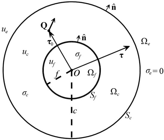
Figure 1. The liquid core model of the brain with the geometrical and physical properties.

The localized electric activity of the cerebrum tissue is represented by an equivalent current dipole located at the fixed point ${\mathsf{\tau }}_0$ inside the region ${\mathsf{\Omega }}_c$, which is characterized by the dipole moment $Q$ and the primary current density

$$J^p(\mathsf{\tau })=Q\delta (\mathsf{\tau }-{\mathsf{\tau }}_0)$$

(1)

where $\delta$ denotes the Dirac measure. This primary current produces an irrotational electric field $E$, which is represented by the electric potential $u$, i.e.,

$$E(\mathsf{\tau })=-\nabla u(\mathsf{\tau }).$$

(2)

The electric potential, denoted by $u_f$, $u_c$, and $u_e$ in ${\mathsf{\Omega }}_f$, ${\mathsf{\Omega }}_c$, and ${\mathsf{\Omega }}_e$, respectively, satisfies the Poisson equation in the region that includes the source (${\mathsf{\Omega }}_c$) and the Laplace equation in ${\mathsf{\Omega }}_f$ and ${\mathsf{\Omega }}_e$, i.e.,

$$\Delta u_f(\mathsf{\tau })=0, \mathsf{\tau }\in {\mathsf{\Omega }}_f,$$

(3)

$${\sigma }_c\Delta u_c(\mathsf{\tau })=\nabla \cdot J^p(\mathsf{\tau }), \mathsf{\tau }\in {\mathsf{\Omega }}_c,$$

(4)

$$\Delta u_e(\mathsf{\tau })=0, \mathsf{\tau }\in {\mathsf{\Omega }}_e,$$

(5)

while on the boundary surfaces $S_f$ and $S_c$, the electric potential and the normal component of the electric field are continuous

$$u_f(\mathsf{\tau })=u_c(\mathsf{\tau }), \mathsf{\tau }\in S_f,$$

(6)

$${\sigma }_f\frac{\partial }{\partial n}{u}_f(\mathsf{\tau })={\sigma }_c\frac{\partial }{\partial n}{u}_c(\mathsf{\tau }), \mathsf{\tau }\in S_f,$$

(7)

$$u_c(\mathsf{\tau })=u_e(\mathsf{\tau }), \mathsf{\tau }\in S_c,$$

(8)

$$\frac{\partial }{\partial n}{u}_c(\mathsf{\tau })=0, \mathsf{\tau }\in S_c.$$

(9)

In order to obtain a unique solution for the exterior potential problem, we also have the requirement that

$$u_e(\mathsf{\tau })=O\left(\frac{1}{\tau }\right), \tau \to \infty ,$$

(10)

whereas

$$\underset{\left|r\right|\to 0}{\lim }{u}_f\left(r\right)\ne \pm \infty .$$

(11)

Note that, for every $\mathsf{\tau }\in {\mathsf{\Omega }}_f\cup {\mathsf{\Omega }}_c\cup {\mathsf{\Omega }}_e$, the electric potential $u$ can be expressed as

$$\begin{array}{cc}\hfill u(\mathsf{\tau })=& H(f-\tau )u_f(\mathsf{\tau })\hfill \\ & +\left[H(c-\tau )-H(f-\tau )\right]u_c(\mathsf{\tau })\hfill \\ & +H(\tau -c)u_e(\mathsf{\tau }) ,\hfill \end{array}$$

(12)

where

$$H(x)=\{\begin{array}{c}1 , x>0\\ 0 , x\le 0\end{array}$$

(13)

is the Heaviside function.

Furthermore, the primary current $J^p$ induces the volume currents

$$J_f^i(\mathsf{\tau })=-{\sigma }_f\nabla u_f(\mathsf{\tau }), \mathsf{\tau }\in {\mathsf{\Omega }}_f$$

(14)

and

$$J_c^i(\mathsf{\tau })=-{\sigma }_c\nabla u_c(\mathsf{\tau }), \mathsf{\tau }\in {\mathsf{\Omega }}_c,$$

(15)

in the conductive regions ${\mathsf{\Omega }}_f$ and ${\mathsf{\Omega }}_c$, respectively, resulting in the total current density

$$J^t(\mathsf{\tau })=J^p(\mathsf{\tau })+J_f^i(\mathsf{\tau })+J_c^i(\mathsf{\tau }).$$

(16)

The total current $J^t$ generates the electric field ${\rm E}$ and the magnetic induction ${\rm B}$ in both the interior and the exterior space, which satisfy the quasi-static approximation of Maxwell’s equations [26]

$$\nabla \times E=0, \nabla \cdot E=0$$

(17)

$$\nabla \times B={\mu }_0{J}^t, \nabla \cdot B=0.$$

(18)

3. The Electric Potential

The electric potential solves the system of mixed boundary value problems (3)–(11). This can be split into three separate problems (3), (4), and (5), subject to the boundary conditions (6)–(9) and the limiting conditions (10) and (11), where we have to deal with the solution of Laplace and Poisson equations in spherical coordinates. To this end, we will use the general expansion of the harmonic function $u$ ($\Delta u=0$)

$$u(\mathsf{\tau })\equiv u(\tau ,\vartheta ,\phi )={\displaystyle \sum _{n=0}^{\infty }{\displaystyle \sum _{m=-n}^n\left[A_n^m{\tau }^n+B_n^m{\tau }^{-(n+1)}\right]Y_n^m\left(\vartheta ,\phi \right)}},$$

(19)

where $A_n^m$ and $B_n^m$, for every $n\ge 0$ and $m=-n,-n+1,\dots ,n-1,n$, are arbitrary constants and $Y_n^m$ are the complex spherical harmonics

$$Y_n^m\left(\vartheta ,\phi \right)={\ell }_n^m{P}_n^{\left|m\right|}(\cos \vartheta )e^{im\phi }$$

(20)

which satisfy the orthonormality relation

$${\displaystyle \underset{0}{\overset{2\pi }{\int }}{\displaystyle \underset{0}{\overset{\pi }{\int }}{Y}_n^m\left(\vartheta ,\phi \right){\overline{Y}}_{n^{\prime }}^{m^{\prime }}\left(\vartheta ,\phi \right)\sin \vartheta d\vartheta d\phi =}}{\delta }_{n{n}^{\prime }}{\delta }_{m{m}^{\prime }},$$

(21)

where $n\ge 0$, $m=-n,-n+1,\dots ,n-1,n$ and

$${\ell }_n^m=\sqrt{\frac{2n+1}{4\pi }\frac{(n-|m|)!}{(n+|m|)!}},$$

(22)

while $P_n^m$ denotes the associated Legendre polynomials and $Y_n^{-m}(\vartheta ,\phi )={(-1)}^m{\overline{Y}}_n^m(\vartheta ,\phi )$.

In the first place, Equation (3) represents the harmonic electric potential in the interior region ${\mathsf{\Omega }}_f$ and, since it refers to an interior BVP that includes the origin, expansion (19) via the condition (11) yields

$$u_f(\mathsf{\tau })={\displaystyle \sum _{n=0}^{\infty }{\displaystyle \sum _{m=-n}^n{A}_{n,f}^m{\tau }^n{Y}_n^m\left(\vartheta ,\phi \right)}}, \mathsf{\tau }\in {\mathsf{\Omega }}_f.$$

(23)

Next, Equation (5) represents the harmonic electric potential in the exterior region ${\mathsf{\Omega }}_e$; hence, as it refers to an exterior problem, utilizing (19) together with (10) gives

$$u_e(\mathsf{\tau })={\displaystyle \sum _{n=0}^{\infty }{\displaystyle \sum _{m=-n}^n{B}_{n,e}^m{\tau }^{-(n+1)}{Y}_n^m\left(\vartheta ,\phi \right)}}, \mathsf{\tau }\in {\mathsf{\Omega }}_e,$$

(24)

where the term for $n=0$ falls as $1/\tau$, which is consistent with condition (10).

Nevertheless, the solution of the Poisson equation (4) is not straightforward. Namely, its solution is a superposition of a harmonic function $u_{c,h}$ and a particular solution $u_{c,p}$ that satisfies (4), i.e.,

$$u_c=u_{c,h}+u_{c,p},$$

(25)

where

$$\Delta u_{c,h}=0$$

(26)

and

$$\begin{array}{c}{\sigma }_c\Delta u_{c,p}(\mathsf{\tau };{\mathsf{\tau }}_0)=\nabla \cdot \left(Q\delta (\mathsf{\tau }-{\mathsf{\tau }}_0)\right)\\ =Q\cdot \nabla \delta (\mathsf{\tau }-{\mathsf{\tau }}_0).\end{array}$$

(27)

Equation (26) is a classical Laplace equation that refers to the intermediate region ${\mathsf{\Omega }}_c$; therefore, it has the general solution (19), which is

$$u_{c,h}(\mathsf{\tau })={\displaystyle \sum _{n=0}^{\infty }{\displaystyle \sum _{m=-n}^n\left[A_{n,c}^m{\tau }^n+B_{n,c}^m{\tau }^{-(n+1)}\right]Y_n^m\left(\vartheta ,\phi \right)}}.$$

(28)

On the other hand, in view of Equation (27), applying the operator $Q\cdot \nabla$ to the two parts of the equation

$$\Delta \left[-\frac{1}{4\pi |\mathsf{\tau }-{\mathsf{\tau }}_0|}\right]=\delta (\mathsf{\tau }-{\mathsf{\tau }}_0),$$

(29)

we are led to the particular solution

$$u_{c,p}(\mathsf{\tau };{\mathsf{\tau }}_0)=-\frac{1}{4\pi {\sigma }_c}Q\cdot \nabla \frac{1}{|\mathsf{\tau }-{\mathsf{\tau }}_0|},$$

(30)

or

$$u_{c,p}(\mathsf{\tau };{\mathsf{\tau }}_0)=\frac{1}{4\pi {\sigma }_c}Q\cdot \frac{\mathsf{\tau }-{\mathsf{\tau }}_0}{|\mathsf{\tau }-{\mathsf{\tau }}_0{|}^3}.$$

(31)

Then, we utilize the formula

$$\frac{1}{|\mathsf{\tau }-{\mathsf{\tau }}_0|}={\displaystyle \sum _{n=0}^{\infty }\frac{{\tau }_{<}^n}{{\tau }_{>}^{n+1}}{\displaystyle \sum _{m=-n}^n\frac{(n-|m|)!}{(n+|m|)!}}}{P}_n^{\left|m\right|}(\cos \vartheta )P_n^{\left|m\right|}(\cos {\vartheta }_0)e^{im(\phi -{\phi }_0)}, \mathsf{\tau }\in {ℝ}^3-\left\{{\mathsf{\tau }}_0\right\},$$

(32)

where

$$\frac{{\tau }_{<}^n}{{\tau }_{>}^{n+1}}={\tau }^{\nu }{\tau }_0^{-(\nu +1)} , \mathrm{with} \nu =\{\begin{array}{c}n , \tau <{\tau }_0\hfill \\ -(n+1) , \tau >{\tau }_0\end{array}$$

(33)

from which we deduce that the fundamental solution of the Laplacian has the following expansion in terms of spherical harmonics

$$\frac{1}{|\mathsf{\tau }-{\mathsf{\tau }}_0|}=4\pi {\displaystyle \sum _{n=0}^{\infty }{\displaystyle \sum _{m=-n}^n\frac{1}{2n+1}\left[{\tau }_0^{-(\nu +1)}{\overline{Y}}_n^m({\vartheta }_0,{\phi }_0)\right]\left[{\tau }^{\nu }{Y}_n^m(\vartheta ,\phi )\right]}}$$

(34)

or

$$\frac{1}{|\mathsf{\tau }-{\mathsf{\tau }}_0|}={\displaystyle \sum _{n=0}^{\infty }{\displaystyle \sum _{m=-n}^n{g}_{n,{ }_{>}^{<}}^m({\mathsf{\tau }}_0)\left[{\tau }^{\nu }{Y}_n^m(\vartheta ,\phi )\right]}},$$

(35)

where

$$g_{n,{ }_{>}^{<}}^m({\mathsf{\tau }}_0)=\frac{4\pi }{2n+1}\left[{\tau }_0^{-(\nu +1)}{\overline{Y}}_n^m({\vartheta }_0,{\phi }_0)\right],$$

(36)

for every $n\ge 0$, $\left|m\right|\le n$, while $\nu$ depends upon the position $\mathsf{\tau }=(\tau ,\vartheta ,\phi )$ over the point ${\mathsf{\tau }}_0=({\tau }_0,{\vartheta }_0,{\phi }_0)$ according to (33). As a result, and bearing in mind that, in general, the operators $\Delta$ and $\nabla$ act on the position vector $\mathsf{\tau }$ (unless otherwise specified) and considering the identity

$$\nabla \frac{1}{|\mathsf{\tau }-{\mathsf{\tau }}_0|}=-{\nabla }_{{\mathsf{\tau }}_0}\frac{1}{|\mathsf{\tau }-{\mathsf{\tau }}_0|},$$

(37)

the particular solution (30), in view of (35), (36), and (37), is written

$$u_{c,p}(\mathsf{\tau };{\mathsf{\tau }}_0)={\displaystyle \sum _{n=0}^{\infty }{\displaystyle \sum _{m=-n}^n{G}_{n,{ }_{>}^{<}}^m({\mathsf{\tau }}_0){\tau }^{\nu }{Y}_n^m(\vartheta ,\phi )}},$$

(38)

where

$$G_{n,{ }_{>}^{<}}^m({\mathsf{\tau }}_0)=\frac{1}{{\sigma }_c(2n+1)}Q\cdot {\nabla }_{{\mathsf{\tau }}_0}\left[{\tau }_0^{-(\nu +1)}{\overline{Y}}_n^m({\vartheta }_0,{\phi }_0)\right],$$

(39)

for every $n\ge 0$, $\left|m\right|\le n$. Therefore, the sought-out solution (25) of the Poisson equation (4), in view of (28) and (38), is written as

$$u_c(\mathsf{\tau })={\displaystyle \sum _{n=0}^{\infty }{\displaystyle \sum _{m=-n}^n\left[A_{n,c}^m{\tau }^n+B_{n,c}^m{\tau }^{-(n+1)}+G_{n,{ }_{>}^{<}}^m({\mathsf{\tau }}_0){\tau }^{\nu }\right]Y_n^m(\vartheta ,\phi )}}, \mathsf{\tau }\in {\mathsf{\Omega }}_c.$$

(40)

Subsequently, we proceed to the calculation of the unknown coefficients $A_{n,f}^m$, $B_{n,e}^m$ and $A_{n,c}^m$, $B_{n,c}^m$ of the expansions (23), (24), and (40), respectively, for every $n\ge 0$ and $\left|m\right|\le n$, utilizing the continuity conditions (6)–(9) and the orthogonality relation (21). In particular, substituting (23) and (40) in (6), for $\tau =f$ and in light of (33), we get

$$\begin{array}{cc}\hfill {\displaystyle \sum _{n=0}^{\infty }{\displaystyle \sum _{m=-n}^n{f}^n{A}_{n,f}^m{Y}_n^m\left(\vartheta ,\phi \right)}}=& {\displaystyle \sum _{n=0}^{\infty }{\displaystyle \sum _{m=-n}^n[f^n{A}_{n,c}^m}}+f^{-(n+1)}{B}_{n,c}^m\hfill \\ & +f^n{G}_{n, <}^m({\mathsf{\tau }}_0)]Y_n^m(\vartheta ,\phi ),\hfill \end{array}$$

(41)

which, by virtue of (21), leads to the equation

$$f^{2n+1}{A}_{n,f}^m-f^{2n+1}{A}_{n,c}^m-B_{n,c}^m=f^{2n+1}{G}_{n, <}^m({\mathsf{\tau }}_0),$$

(42)

for every $n\ge 0$, $\left|m\right|\le n$.

Next, from (7), (23) and (40), we have ($\partial /\partial n=\widehat{n}\cdot \nabla \equiv \partial /\partial \tau$ on $S_f$, $S_c$)

$$\begin{array}{cc}{\sigma }_f{\displaystyle \sum _{n=0}^{\infty }{\displaystyle \sum _{m=-n}^{n}n{f}^{n-1}{A}_{n,f}^m{Y}_n^m\left(\vartheta ,\phi \right)}}=& {\sigma }_c{\displaystyle \sum _{n=0}^{\infty }{\displaystyle \sum _{m=-n}^n[n{f}^{n-1}{A}_{n,c}^m}}-(n+1)f^{-(n+2)}{B}_{n,c}^m\hfill \\ & +n{f}^{n-1}{G}_{n, <}^m({\mathsf{\tau }}_0)]Y_n^m(\vartheta ,\phi ),\hfill \end{array}$$

(43)

which yields

$$\frac{{\sigma }_f}{{\sigma }_c}\frac{n}{n+1}{f}^{2n+1}{A}_{n,f}^m-\frac{n}{n+1}{f}^{2n+1}{A}_{n,c}^m+B_{n,c}^m=\frac{n}{n+1}{f}^{2n+1}{G}_{n, <}^m({\mathsf{\tau }}_0),$$

(44)

for every $n\ge 0$, $\left|m\right|\le n$.

Similarly, for $\tau =c$ and in view of (33) and (21), condition (8) with (24) and (40) leads to

$$c^{2n+1}{A}_{n,c}^m+B_{n,c}^m-B_{n,e}^m=-G_{n, >}^m({\mathsf{\tau }}_0),$$

(45)

for every $n\ge 0$, $\left|m\right|\le n$, while from (9) and (40), we have

$$\frac{n}{n+1}{c}^{2n+1}{A}_{n,c}^m-B_{n,c}^m=G_{n, >}^m({\mathsf{\tau }}_0),$$

(46)

for every $n\ge 0$, $\left|m\right|\le n$.

In conclusion, the coefficients of the expansions (23), (24), and (40) are given by the solution of the $4\times 4$ linear system (42), (44), (45), and (46), i.e.,

$$A_{n,f}^m=\frac{b_n^m}{D_n},$$

(47)

$$A_{n,c}^m={\sigma }_n\frac{b_n^m}{D_n}-G_{n, <}^m({\mathsf{\tau }}_0),$$

(48)

$$B_{n,c}^m=b_n^m{f}^{2n+1}\left(\frac{a_n{\sigma }_n}{D_n}-1\right),$$

(49)

$$B_{n,e}^m=\frac{2n+1}{n+1}{c}^{2n+1}\left(\frac{b_n^m{\sigma }_n}{D_n}-G_{n, <}^m({\mathsf{\tau }}_0)\right),$$

(50)

where

$$D_n=\left(1+a_n\right){\sigma }_n-1,$$

(51)

$$b_n^m=f^{-(2n+1)}{G}_{n, >}^m({\mathsf{\tau }}_0)+a_n{G}_{n, <}^m({\mathsf{\tau }}_0),$$

(52)

$$a_n=\frac{n}{n+1}{a}^{2n+1}, {\sigma }_n=\frac{(\sigma +1)n+1}{2n+1} \mathrm{and} a=\frac{c}{f}>1, \sigma =\frac{{\sigma }_f}{{\sigma }_c}$$

(53)

for every $n\ge 1$, $\left|m\right|\le n$.

The special case for $n=0$ ($m=0$) must be treated separately, since $D_0=0$ (note that $a_0={\sigma }_0=0$) in the dominators of (47)–(50), providing

$$\frac{B_{0,e}^0}{c}=A_{0,c}^0=A_{0,f}^0+\frac{1}{4\pi {\sigma }_c}\frac{Q\cdot {\widehat{\mathsf{\tau }}}_0}{{\tau }_0^2} \mathrm{and} B_{0,c}^0=0, \mathrm{where} A_{0,f}^0\in ℝ,$$

(54)

which concludes the analytical solution of the problem. At this point, we are obliged to make a crucial remark with respect to the undetermined constant coefficient $A_{0,f}^0\in ℝ$ (the rest of the constants are given in terms of $A_{0,f}^0$) that reflects the lack of uniqueness for our problem [15], which is actually due to the fact that Neumann-type conditions are incorporated into the boundary value problem under consideration. As a matter of fact, this is not the case herein, and uniqueness is secured since the interior electric potential (23) is written in terms of the additive constant $A_{0,f}^0$, arising from the case $n=0$, which vanishes when the Neumann condition applies, while all the other coefficients are evaluated explicitly. However, it is obvious that an additional condition must be imposed in order to calculate this coefficient, which could be the assignment of a specific value for the potential $u_f$ at $\tau =0$ through the general condition (11). For example, the choice $u_f(0)=0$ fixes the arbitrary additional constant, allowed by the mathematical statement of the problem, i.e., $A_{0,f}^0=0$. Therefore, this peculiarity of the forward EEG problem that appears in the literature is evidently treatable, leading to uniqueness in that sense, and the given solution holds true.

4. The Single Compartment Limiting Case

In this section, we consider the limiting case where the concentric fluid core vanishes. Then, obviously, the only remaining fields are $u_c$ and $u_e$, where we have $f\to 0^{+}$, hence, for $n\ge 1$, $\{a,a_n,D_n\}\to +\infty$, while $D_n=a_n$, assuming ${\sigma }_f={\sigma }_c$, therefore $\sigma =1$ and ${\sigma }_n=1$. In this particular case, the coefficient (47) does not correspond to a field; however, it is integrated into the coefficients (48)–(50). Hence, provided that the source functions $G_{n,{ }_{<}^{>}}^m({\mathsf{\tau }}_0)$ are bounded, relation (52) gives $b_n^m\to \pm \infty$ and (47) takes the form

$$A_{n,f}^m=\frac{n+1}{n}{c}^{-(2n+1)}{G}_{n, >}^m({\mathsf{\tau }}_0)+G_{n, <}^m({\mathsf{\tau }}_0),$$

(55)

for every $n\ge 1$, $\left|m\right|\le n$.

As a result, (48) becomes

$$A_{n,c}^m=\frac{n+1}{n}{c}^{-(2n+1)}{G}_{n, >}^m({\mathsf{\tau }}_0),$$

(56)

for every $n\ge 1$, $\left|m\right|\le n$.

On the other hand, since $D_n=a_n{\sigma }_n$, from (49), it turns out that

$$B_{n,c}^m=0,$$

(57)

for every $n\ge 0$, $\left|m\right|\le n$, which is expected as the intermediate cell problem in ${\mathsf{\Omega }}_c$ has now become an interior one (the corresponding expansion does not contain the term ${\tau }^{-(n+1)}$ for all $n\ge 0$).

Then, since ${\sigma }_n=1$, from (50), we end up to

$$B_{n,e}^m=\frac{2n+1}{n}{G}_{n, >}^m({\mathsf{\tau }}_0),$$

(58)

for every $n\ge 1$, $\left|m\right|\le n$.

Finally, for $n=0$ and $m=0$, due to (54), we obtain

$$\frac{B_{0,e}^0}{c}=A_{0,c}^0=A_{0,f}^0+\frac{1}{4\pi {\sigma }_c}\frac{Q\cdot {\widehat{\mathsf{\tau }}}_0}{{\tau }_0^2}, \mathrm{where} A_{0,f}^0\in ℝ,$$

(59)

which inherits the lack of uniqueness of the Neumann-type boundary value problem and the necessity of additional information, as is readily discussed in the previous section. The result (59) does not cancel either (56) or (58) since they both always hold true, providing zero on each side, due to the fact that $G_{0, >}^0({\mathsf{\tau }}_0)=0$ from (39) with (33).

To sum up, in this instance, the involved potentials $u_e$ and $u_c$ are derived from (24) and (40), respectively, i.e.,

$$u_e(\mathsf{\tau })={\displaystyle \sum _{n=0}^{\infty }{\displaystyle \sum _{m=-n}^n{B}_{n,e}^m{\tau }^{-(n+1)}{Y}_n^m\left(\vartheta ,\phi \right)}}$$

(60)

and

$$u_c(\mathsf{\tau })={\displaystyle \sum _{n=0}^{\infty }{\displaystyle \sum _{m=-n}^n\left[A_{n,c}^m{\tau }^n+G_{n,{ }_{>}^{<}}^m({\mathsf{\tau }}_0){\tau }^{\nu }\right]Y_n^m(\vartheta ,\phi )}},$$

(61)

where the coefficients are given by (56), (58), and (59), while we utilize (39) according to definition (33). The potential fields (60) and (61) coincide with those in the bibliography for the single-layer spherical model, providing an effective analytical validation of our analytical approach.

5. Numerical Implementation and Results

For the purpose of illustrating the above analytical results and investigating the usefulness of the presented model, we provide a graph (see Figure 2) of the electric potential on the surface of the head, where we consider a dipole $Q=(2,1,3)\times {10}^{-5}\mathrm{Cm}$, situated inside the cerebrum ${\mathsf{\Omega }}_c$, at a point with coordinates ${\tau }_0=5 \mathrm{cm}$, ${\vartheta }_0=\pi /3$ and ${\phi }_0=4\pi /3$. Moreover, we assume that the cerebrum has an outer radius $c=7 \mathrm{cm}$ and electric conductivity ${\sigma }_c=0.37 \mathrm{S}/\mathrm{m}$ [16], while we consider the interior region ${\mathsf{\Omega }}_f$ with a higher conductivity ${\sigma }_f=1.6 \mathrm{S}/\mathrm{m}$ and three different radii: (a) $f=4.95 \mathrm{cm}$, (b) $f=3.8 \mathrm{cm}$, and (c) $f=0.1 \mathrm{cm}$. The surface electric potential was calculated with a sufficient degree of accuracy, utilizing expansion (24) for $\tau =c$ and for $n$ up to $n_{\max }=25$ (see Figure 3), considering a value of $A_{0,f}^0={10}^{-4}\mathrm{V}$.

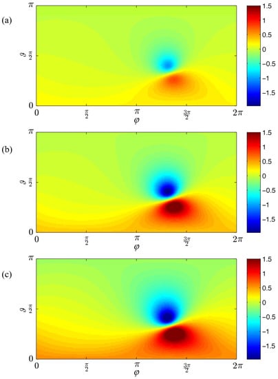
Figure 2. The surface electric potential (in ${10}^{-2}\mathrm{V}$) for the two-compartment brain swelling model, given a current dipole with $Q=(2,1,3)\times {10}^{-5}\mathrm{Cm}$, located at ${\tau }_0=5 \mathrm{cm}$, ${\vartheta }_0=\pi /3$, and ${\phi }_0=4\pi /3$, considering three cases of the liquid core with radii: (a) $f=4.95 \mathrm{cm}$, (b) $f=3.8 \mathrm{cm}$, and (c) $f=0.1 \mathrm{cm}$.

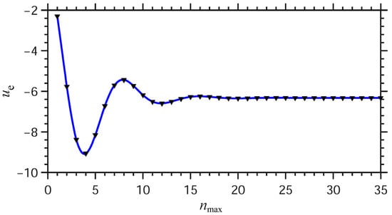
Figure 3. Convergence of the expansion of the exterior potential $u_e$ (in ${10}^{-3}\mathrm{V}$) on a specific point of the external surface $S_c$ $(\tau ,\vartheta ,\phi )=(c, 7\pi /12,4\pi /3)$, where $c=7\mathrm{cm}$ and the radius of the fluid core is $f=3.8 \mathrm{cm}$.

Indeed, the corresponding Figure 2 (a), (b), and (c) verify that the presence of an adequately large edema, with different electric conductivity than that of the cerebrum, influences EEG recordings. The differences between cases (a), (b), and (c) are evident in the whole surface of the head, depending on the size of the fluid core, although they seem to be stronger around the peak values of the potential, e.g., along the direction of the current dipole $({\vartheta }_0=\pi /3, {\phi }_0=4\pi /3)$. However, numerical experiments showed that the differences between these three cases become inconsiderable if we assume a value of ${\sigma }_f$ close to that of ${\sigma }_c$, which is expected. Note that the third case (c) almost represents the limiting case analyzed in Section 4, where the fluid core is nonexistent.

As it is demonstrated in Figure 3, the exterior potential $u_e$ on a specific point of external surface $S_c$ starts to converge after the use of about 15 terms for $n$ in the expansion of the potential (24), i.e., $n_{\max }=15$. However, in order to be consistent with high accuracy in practical situations, in Figure 2, we utilized $n_{\max }=25$, wherein the use of additional terms does not contribute to the values of the potential.

6. The Magnetic Field

The magnetic induction field is obtained by employing the Biot-Savart law

$$B(\mathsf{\tau };{\mathsf{\tau }}_0)=\frac{{\mu }_0}{4\pi }{\displaystyle \underset{\mathsf{\Omega }}{\int }{J}^t({\mathsf{\tau }}^{\prime };{\mathsf{\tau }}_0)}\times \frac{\mathsf{\tau }-{\tau }^{\prime }}{|\mathsf{\tau }-{\mathsf{\tau }}^{\prime }{|}^3}dV({\mathsf{\tau }}^{\prime }),$$

(62)

where $\mathsf{\Omega }$ denotes the support of the total current $J^t$. Substituting (16) in (62) leads to

$$\begin{array}{cc}\hfill B(\mathsf{\tau };{\mathsf{\tau }}_0)=& \frac{{\mu }_0}{4\pi }Q\times \frac{\mathsf{\tau }-{\mathsf{\tau }}_0}{|\mathsf{\tau }-{\mathsf{\tau }}_0{|}^3}-\frac{{\mu }_0{\sigma }_f}{4\pi }{\displaystyle \underset{{\mathsf{\Omega }}_f}{\int }{\nabla }_{{\mathsf{\tau }}^{\prime }} u_f({\mathsf{\tau }}^{\prime })}\times \frac{\mathsf{\tau }-{\mathsf{\tau }}^{\prime }}{|\mathsf{\tau }-{\mathsf{\tau }}^{\prime }{|}^3}dV({\mathsf{\tau }}^{\prime }) \hfill \\ & -\frac{{\mu }_0{\sigma }_c}{4\pi }{\displaystyle \underset{{\mathsf{\Omega }}_c}{\int }{\nabla }_{{\mathsf{\tau }}^{\prime }} u_c({\mathsf{\tau }}^{\prime })}\times \frac{\mathsf{\tau }-{\mathsf{\tau }}^{\prime }}{|\mathsf{\tau }-{\mathsf{\tau }}^{\prime }{|}^3}dV({\mathsf{\tau }}^{\prime }),\hfill \end{array}$$

(63)

which is valid for every $\mathsf{\tau }$ in the interior and the exterior space. Now, we proceed with the application of the divergence theorem [9,27] in the regions ${\mathsf{\Omega }}_f$ and ${\mathsf{\Omega }}_c$, bearing in mind that ${\mathsf{\Omega }}_c$ is a spherical shell enclosed between the surfaces $S_f$ and $S_c$. Then, the volume integrals become surface integrals and (63) leads to Geselowitz’s formula (valid for all $\mathsf{\tau }$, except those on the surfaces $S_f$ and $S_c$ [9])

$$\begin{array}{cc}\hfill B(\mathsf{\tau };{\mathsf{\tau }}_0)=& \frac{{\mu }_0}{4\pi }Q\times \frac{\mathsf{\tau }-{\mathsf{\tau }}_0}{|\mathsf{\tau }-{\mathsf{\tau }}_0{|}^3}-\frac{{\mu }_0{\sigma }_c}{4\pi }{\displaystyle \underset{S_c}{\int }{u}_c({\mathsf{\tau }}^{\prime })} {\widehat{n}}^{\prime }\times \frac{\mathsf{\tau }-{\mathsf{\tau }}^{\prime }}{|\mathsf{\tau }-{\mathsf{\tau }}^{\prime }{|}^3}dS({\mathsf{\tau }}^{\prime }) \hfill \\ & +\frac{{\mu }_0}{4\pi }{\displaystyle \underset{S_f}{\int }\left({\sigma }_c{u}_c({\mathsf{\tau }}^{\prime })-{\sigma }_f{u}_f({\mathsf{\tau }}^{\prime })\right)} {\widehat{n}}^{\prime }\times \frac{\mathsf{\tau }-{\mathsf{\tau }}^{\prime }}{|\mathsf{\tau }-{\mathsf{\tau }}^{\prime }{|}^3}dS({\mathsf{\tau }}^{\prime }).\hfill \end{array}$$

(64)

Due to the spherical symmetry of the present model, in every point of the concentric spherical surfaces $S_f$ and $S_c$, the outwardly directed unit normal ${\widehat{n}}^{\prime }$ coincides with the radial unit vector ${\widehat{\mathsf{\tau }}}^{\prime }$, i.e.,

$${\widehat{n}}^{\prime }=\widehat{n}({\mathsf{\tau }}^{\prime })\equiv {\widehat{\mathsf{\tau }}}^{\prime },$$

(65)

hence, in view of the identity

$$\frac{\mathsf{\tau }-{\mathsf{\tau }}^{\prime }}{|\mathsf{\tau }-{\mathsf{\tau }}^{\prime }{|}^3}={\nabla }_{{\mathsf{\tau }}^{\prime }}\frac{1}{|\mathsf{\tau }-{\mathsf{\tau }}^{\prime }|}\equiv -{\nabla }_{\mathsf{\tau }}\frac{1}{|\mathsf{\tau }-{\mathsf{\tau }}^{\prime }|},$$

(66)

relation (64) yields

$$\begin{array}{cc}\hfill B(\mathsf{\tau };{\mathsf{\tau }}_0)=& \frac{{\mu }_0}{4\pi }Q\times \frac{\mathsf{\tau }-{\mathsf{\tau }}_0}{|\mathsf{\tau }-{\mathsf{\tau }}_0{|}^3}-\frac{{\mu }_0{\sigma }_c}{4\pi }{\displaystyle \underset{S_c}{\int }{u}_c({\mathsf{\tau }}^{\prime })} {\widehat{\mathsf{\tau }}}^{\prime }\times {\nabla }_{{\mathsf{\tau }}^{\prime }}\frac{1}{|\mathsf{\tau }-{\mathsf{\tau }}^{\prime }|}dS({\mathsf{\tau }}^{\prime }) \hfill \\ & +\frac{{\mu }_0}{4\pi }{\displaystyle \underset{S_f}{\int }\left({\sigma }_c{u}_c({\mathsf{\tau }}^{\prime })-{\sigma }_f{u}_f({\mathsf{\tau }}^{\prime })\right)} {\widehat{\mathsf{\tau }}}^{\prime }\times {\nabla }_{{\mathsf{\tau }}^{\prime }}\frac{1}{|\mathsf{\tau }-{\mathsf{\tau }}^{\prime }|}dS({\mathsf{\tau }}^{\prime }),\hfill \end{array}$$

(67)

where

$${\nabla }_{{\mathsf{\tau }}^{\prime }}={\widehat{\mathsf{\tau }}}^{\prime }\frac{\partial }{\partial {\tau }^{\prime }}+\frac{1}{{\tau }^{\prime }}{\widehat{\theta }}^{\prime }\frac{\partial }{\partial {\vartheta }^{\prime }}+\frac{1}{{\tau }^{\prime }\sin {\vartheta }^{\prime }}{\widehat{\phi }}^{\prime }\frac{\partial }{\partial {\phi }^{\prime }}$$

(68)

and

$${\widehat{\mathsf{\tau }}}^{\prime }=\left(\cos {\vartheta }^{\prime },\sin {\vartheta }^{\prime }\cos {\phi }^{\prime },\sin {\vartheta }^{\prime }\sin {\phi }^{\prime }\right),$$

(69)

$${\widehat{\theta }}^{\prime }=\left(-\sin {\vartheta }^{\prime },\cos {\vartheta }^{\prime }\cos {\phi }^{\prime },\cos {\vartheta }^{\prime }\sin {\phi }^{\prime }\right),$$

(70)

$${\widehat{\phi }}^{\prime }=\left(0,-\sin {\phi }^{\prime },\cos {\phi }^{\prime }\right).$$

(71)

for every ${\vartheta }^{\prime }\in [0,\pi ]$ and ${\phi }^{\prime }\in [0,2\pi )$.

We also remind from (35) that

$$\frac{1}{|\mathsf{\tau }-{\mathsf{\tau }}^{\prime }|}={\displaystyle \sum _{n=0}^{\infty }{\displaystyle \sum _{m=-n}^n{g}_{n,{ }_{>}^{<}}^m}}({\mathsf{\tau }}^{\prime })\left[{\tau }^{\nu }{Y}_n^m(\vartheta ,\phi )\right],$$

(72)

where

$$g_{n,{ }_{>}^{<}}^m({\mathsf{\tau }}^{\prime })=\frac{4\pi }{2n+1}\left[{{\tau }^{\prime }}^{-(\nu +1)}{\overline{Y}}_n^m({\vartheta }^{\prime },{\phi }^{\prime })\right],$$

(73)

for every $n\ge 0$ and $\left|m\right|\le n$, while

$$\nu =\{\begin{array}{c}n \mathrm{and} “ < ”, \tau <{\tau }^{\prime }\hfill \\ -(n+1) \mathrm{and} “ > ”, \tau >{\tau }^{\prime }\end{array} , n\ge 0,$$

(74)

depends upon the position $\mathsf{\tau }$ over the point $({\tau }^{\prime },{\vartheta }^{\prime },{\phi }^{\prime })$. Moreover, the potentials $u_f$ and $u_c$ are given by (23) and (40), respectively, which can be rewritten as

$$u_f({\mathsf{\tau }}^{\prime })={\displaystyle \sum _{n=0}^{\infty }{\displaystyle \sum _{m=-n}^n{A}_{n,f}^m{{\tau }^{\prime }}^n{Y}_n^m\left({\vartheta }^{\prime },{\phi }^{\prime }\right)}}$$

(75)

and

$$u_c({\mathsf{\tau }}^{\prime })={\displaystyle \sum _{n=0}^{\infty }{\displaystyle \sum _{m=-n}^n\left[A_{n,c}^m{{\tau }^{\prime }}^n+B_{n,c}^m{{\tau }^{\prime }}^{-(n+1)}+G_{n,{ }_{>}^{<}}^m({\mathsf{\tau }}_0){{\tau }^{\prime }}^{\nu }\right]Y_n^m({\vartheta }^{\prime },{\phi }^{\prime })}}.$$

(76)

Finally, taking the dot product of (67) and $\widehat{\mathsf{\tau }}$ and provided that

$$\widehat{\mathsf{\tau }}\cdot {\widehat{\mathsf{\tau }}}^{\prime }\times {\nabla }_{{\mathsf{\tau }}^{\prime }}\frac{1}{|\mathsf{\tau }-{\mathsf{\tau }}^{\prime }|}=\widehat{\mathsf{\tau }}\cdot {\widehat{\mathsf{\tau }}}^{\prime }\times \frac{\tau \widehat{\mathsf{\tau }}}{|\mathsf{\tau }-{\mathsf{\tau }}^{\prime }{|}^3}-\widehat{\mathsf{\tau }}\cdot {\widehat{\mathsf{\tau }}}^{\prime }\times \frac{{\tau }^{\prime }{\widehat{\mathsf{\tau }}}^{\prime }}{|\mathsf{\tau }-{\mathsf{\tau }}^{\prime }{|}^3}=0,$$

(77)

the involved surface integrals vanish, therefore we end up to

$$\widehat{\mathsf{\tau }}\cdot B(\mathsf{\tau };{\mathsf{\tau }}_0)=-\frac{{\mu }_0}{4\pi }\frac{Q\times {\mathsf{\tau }}_0\cdot \widehat{\mathsf{\tau }}}{|\mathsf{\tau }-{\mathsf{\tau }}_0{|}^3},$$

(78)

which is valid for every $\mathsf{\tau }$ and means that the radial component of $B$ is a function of only the dipole moment $Q$ and its location ${\mathsf{\tau }}_0$. This is an important result, which has been proved in [9], according to which MEG is independent of any radial variation of the conductivity in a spherical model, which means that it does not depend on the edema region.

7. The Exterior Magnetic Field

Next, we calculate $B$ in the exterior space ${\mathsf{\Omega }}_e$ where the total current $J^t$ is zero; hence, (18) implies that the magnetic field is both irrotational and solenoidal. Therefore, it accepts the representation

$$B(\mathsf{\tau };{\mathsf{\tau }}_0)=\frac{{\mu }_0}{4\pi }\nabla U(\mathsf{\tau };{\mathsf{\tau }}_0) , \mathrm{with} \Delta U(\mathsf{\tau };{\mathsf{\tau }}_0)=0,$$

(79)

for every $\mathsf{\tau }\in {\mathsf{\Omega }}_e$. Now, since the magnetic scalar potential $U$ in the exterior space has the asymptotic behavior

$$U(\mathsf{\tau };{\mathsf{\tau }}_0)=O\left(\frac{1}{{\tau }^2}\right), \tau \to \infty ,$$

(80)

we obtain

$$\begin{array}{cc}\hfill U(\mathsf{\tau };{\mathsf{\tau }}_0)& =-{\displaystyle \underset{\tau }{\overset{+\infty }{\int }}\frac{\partial }{\partial {\tau }^{\prime }}}U({\mathsf{\tau }}^{\prime };{\mathsf{\tau }}_0)d{\tau }^{\prime }\hfill \\ & =-{\displaystyle \underset{\tau }{\overset{+\infty }{\int }}{\widehat{\mathsf{\tau }}}^{\prime }\cdot {\nabla }_{{\mathsf{\tau }}^{\prime }}}U({\mathsf{\tau }}^{\prime };{\mathsf{\tau }}_0)d{\tau }^{\prime }, \mathsf{\tau }\in {\mathsf{\Omega }}_e,\hfill \end{array}$$

(81)

hence, from (78) and (79), we arrive at

$$U(\mathsf{\tau };{\mathsf{\tau }}_0)=-\frac{4\pi }{{\mu }_0}{\displaystyle \underset{\tau }{\overset{+\infty }{\int }}{\widehat{\mathsf{\tau }}}^{\prime }\cdot B({\mathsf{\tau }}^{\prime };{\mathsf{\tau }}_0)}d{\tau }^{\prime }, \mathsf{\tau }\in {\mathsf{\Omega }}_e,$$

(82)

or

$$U(\mathsf{\tau };{\mathsf{\tau }}_0)={\displaystyle \underset{\tau }{\overset{+\infty }{\int }}\frac{Q\times {\mathsf{\tau }}_0\cdot {\widehat{\mathsf{\tau }}}^{\prime }}{|{\mathsf{\tau }}^{\prime }-{\mathsf{\tau }}_0{|}^3}}d{\tau }^{\prime }, \mathsf{\tau }\in {\mathsf{\Omega }}_e.$$

(83)

In this case, where ${\rm B}$ is also a conservative field (as irrotational), we can choose to integrate along the radial direction $\widehat{\mathsf{\tau }}$, from $\tau$ to infinity (path independent). Then, the above takes the form

$$U(\mathsf{\tau };{\mathsf{\tau }}_0)=Q\times {\mathsf{\tau }}_0\cdot \widehat{\mathsf{\tau }}{\displaystyle \underset{\tau }{\overset{+\infty }{\int }}\frac{dt}{|t\widehat{\mathsf{\tau }}-{\mathsf{\tau }}_0{|}^3}},$$

(84)

which is written as

$$U(\mathsf{\tau };{\mathsf{\tau }}_0)=\frac{Q\times {\mathsf{\tau }}_0\cdot \mathsf{\tau }}{F(\mathsf{\tau };{\mathsf{\tau }}_0)}, \mathsf{\tau }\in {\mathsf{\Omega }}_e,$$

(85)

where

$$\begin{array}{cc}\hfill F(\mathsf{\tau };{\mathsf{\tau }}_0)& =|\mathsf{\tau }-{\mathsf{\tau }}_0|\left[\tau |\mathsf{\tau }-{\mathsf{\tau }}_0|+\mathsf{\tau }\cdot (\mathsf{\tau }-{\mathsf{\tau }}_0)\right]\hfill \\ & =|\mathsf{\tau }-{\mathsf{\tau }}_0{|}^2\mathsf{\tau }\cdot \left[\widehat{\mathsf{\tau }}+\frac{\mathsf{\tau }-{\mathsf{\tau }}_0}{|\mathsf{\tau }-{\mathsf{\tau }}_0|}\right], \mathsf{\tau }\in {\mathsf{\Omega }}_e.\hfill \end{array}$$

(86)

To conclude, the magnetic induction (79), in view of (85), becomes

$$B(\mathsf{\tau };{\mathsf{\tau }}_0)=\frac{{\mu }_0}{4\pi }\frac{\nabla \left(Q\times {\mathsf{\tau }}_0\cdot \mathsf{\tau }\right)}{F(\mathsf{\tau };{\mathsf{\tau }}_0)}-\frac{{\mu }_0}{4\pi }\left(Q\times {\mathsf{\tau }}_0\cdot \mathsf{\tau }\right)\frac{\nabla F(\mathsf{\tau };{\mathsf{\tau }}_0)}{F^2(\mathsf{\tau };{\mathsf{\tau }}_0)},$$

(87)

where

$$\begin{array}{cc}\hfill \nabla \left(Q\times {\mathsf{\tau }}_0\cdot \mathsf{\tau }\right)& =\nabla \left(Q\times {\mathsf{\tau }}_0\right)\cdot \mathsf{\tau }+Q\times {\mathsf{\tau }}_0\cdot \nabla \mathsf{\tau }\hfill \\ & =Q\times {\mathsf{\tau }}_0\hfill \end{array}$$

(88)

and

$$\begin{array}{cc}\hfill \nabla F(\mathsf{\tau };{\mathsf{\tau }}_0)=& |\mathsf{\tau }-{\mathsf{\tau }}_0|\left(\tau +|\mathsf{\tau }-{\mathsf{\tau }}_0|\right)\widehat{\mathsf{\tau }}\hfill \\ & +\left[|\mathsf{\tau }-{\mathsf{\tau }}_0{|}^2+2\tau |\mathsf{\tau }-{\mathsf{\tau }}_0|+\mathsf{\tau }\cdot (\mathsf{\tau }-{\mathsf{\tau }}_0)\right]\frac{\mathsf{\tau }-{\mathsf{\tau }}_0}{|\mathsf{\tau }-{\mathsf{\tau }}_0|} ,\hfill \end{array}$$

(89)

for every $\mathsf{\tau }\in {\mathsf{\Omega }}_e$, hence,

$$\begin{array}{cc}\hfill B(\mathsf{\tau };{\mathsf{\tau }}_0)=& \frac{{\mu }_0}{4\pi }\frac{Q\times {\mathsf{\tau }}_0}{F(\mathsf{\tau };{\mathsf{\tau }}_0)}-\frac{{\mu }_0}{4\pi }\frac{Q\times {\mathsf{\tau }}_0\cdot \mathsf{\tau }}{F^2(\mathsf{\tau };{\mathsf{\tau }}_0)}[|\mathsf{\tau }-{\mathsf{\tau }}_0|\left(\tau +|\mathsf{\tau }-{\mathsf{\tau }}_0|\right)\widehat{\mathsf{\tau }}\hfill \\ & +\left(|\mathsf{\tau }-{\mathsf{\tau }}_0{|}^2+2\tau |\mathsf{\tau }-{\mathsf{\tau }}_0|+\mathsf{\tau }\cdot (\mathsf{\tau }-{\mathsf{\tau }}_0)\right)\frac{\mathsf{\tau }-{\mathsf{\tau }}_0}{|\mathsf{\tau }-{\mathsf{\tau }}_0|}],\hfill \end{array}$$

(90)

for every $\mathsf{\tau }\in {\mathsf{\Omega }}_e$.

Finally, if we introduce

$$R=\mathsf{\tau }-{\mathsf{\tau }}_0 \mathrm{with} |R|=|\mathsf{\tau }-{\mathsf{\tau }}_0| \mathrm{and} \widehat{R}=\frac{R}{R}=\frac{\mathsf{\tau }-{\mathsf{\tau }}_0}{|\mathsf{\tau }-{\mathsf{\tau }}_0|},$$

(91)

the magnetic potential (85) is written

$$U(\mathsf{\tau };{\mathsf{\tau }}_0)=Q\cdot \frac{\widehat{\mathsf{\tau }}\times \widehat{R}}{R(1+\widehat{\mathsf{\tau }}\cdot \widehat{R})}, \mathsf{\tau }\in {\mathsf{\Omega }}_e,$$

(92)

while the magnetic induction (90) takes the form

$$B(\mathsf{\tau };{\mathsf{\tau }}_0)=\frac{{\mu }_0}{4\pi }\frac{Q\times (\mathsf{\tau }-R)}{\tau R^2(1+\widehat{\mathsf{\tau }}\cdot \widehat{R})}-\frac{{\mu }_0}{4\pi }\frac{Q\cdot \widehat{\mathsf{\tau }}\times \widehat{R}}{R^2(1+\widehat{\mathsf{\tau }}\cdot \widehat{R})}\left[\widehat{R}+\frac{\tau +R}{\tau }\frac{\widehat{\mathsf{\tau }}+\widehat{R}}{1+\widehat{\mathsf{\tau }}\cdot \widehat{R}}\right], \mathsf{\tau }\in {\mathsf{\Omega }}_e.$$

(93)

The above results (85) and (90) or (92) and (93) comprise closed-form representations (that do not depend on ${\sigma }_f,{\sigma }_c$) of the magnetic potential and the magnetic field, respectively, in the exterior of a human head with brain edema, where it is evident that if the point current dipole is radial, the magnetic field vanishes. This is a famous result in MEG research, which can be easily proved with the aid of expression (87). Indeed, a radial dipole assumes the form $Q=Q \widehat{\mathsf{\tau }}$, thus considering that the position vector reads $\mathsf{\tau }=\tau \widehat{\mathsf{\tau }}$, then it is easily shown that $Q\times {\mathsf{\tau }}_0\cdot \mathsf{\tau }=Q \widehat{\mathsf{\tau }}\times {\mathsf{\tau }}_0\cdot \tau \widehat{\mathsf{\tau }}=Q\tau \widehat{\mathsf{\tau }}\times {\mathsf{\tau }}_0\cdot \widehat{\mathsf{\tau }}=0$, since the mixed triple product becomes zero. This outcome is readily substituted to (87), leading to $B(\mathsf{\tau };{\mathsf{\tau }}_0)=0$, which verifies the fact that a radial dipole produces no exterior magnetic field.

Obviously, these results for the exterior magnetic field are identical to the corresponding results of the single-compartment spherical model of the cerebrum (without edema), which frequently appear in the ample literature for EEG and MEG.

8. Conclusions and Discussion

In this work, we provide analytical results for the electric potential and the magnetic field in the interior and the exterior of the head, which is modeled as a non-homogeneous conductor consisting of a spherical fluid core and a concentric spherical shell representing the cerebrum, where the current dipole lies. We observe that the results for the exterior magnetic field are not affected by the existence of the liquid core. However, the interior and exterior electric potential is a function of the fluid core diameter; hence, EEG recordings could be beneficial in confirming the existence of brain swelling. The reduction of the obtained results of the electric potentials for the EEG to those that correspond to the single-layer problem and the evaluation of the exterior magnetic field that is independent of the interior properties of the cerebrum, provide us with already well-known information, which stands for a valuable criterion of the validity of our method.

The advantage of such analytical solutions and closed-type formulae in comparison with pure numerical methodologies lies in the fact that they readily provide efficient and handy expressions for the evaluation of the implicated fields. Therefore, the validity of numerical solutions can be verified by these analytical or even semi-analytical techniques. On the other hand, fundamental physical laws are derived from analytical methods providing a stable and secure basis for starting a numerical procedure. Consequently, simple analytical methods can co-exist with numerical analysis, cooperating toward the solution of boundary value problems in physical applications of importance.

Our future steps involve further and more sophisticated investigation of the above spherical model in terms of an eccentric spherical edema with respect to the center of the brain tissue and/or a multilayer spherical head model, considering the effect of the skull and the scalp (along with the edema and the brain tissue) only to the EEG problem since the MEG problem does not depend on the skull and scalp conductivities. Finally, future work includes extensive numerical evaluation in order to estimate the effect of the size of the fluid core and the location of the dipole source in EEG recordings, as well as the use of computational experiments with the parameters from real life in order to demonstrate the possibilities of the model to reproduce the situations that are interesting for medicine and biophysics.

References

- Arbib, M.A. The Handbook of Brain Theory and Neural Networks; MIT Press: Cambridge, MA, USA, 2003. [Google Scholar]
- Cuffin, B.N.; Cohen, D. Magnetic fields of a dipole in special volume conductor shapes. IEEE Trans. Biomed. Eng. 1977, BME-24, 372–381. [Google Scholar] [CrossRef] [PubMed]
- Geselowitz, D.B. On bioelectric potentials in an inhomogeneous volume conductor. Biophys. J. 1967, 7, 1–11. [Google Scholar] [CrossRef]
- Hamalainen, M.S.; Hari, R.; Ilmoniemi, R.J.; Knuutila, J.; Lounasmaa, O.V. Magnetoencephalographytheory, instrumentation, and applications to noninvasive studies of the working human brain. Rev. Mod. Phys. 1993, 65, 413–497. [Google Scholar] [CrossRef]
- Malmivuo, J.; Plonsey, R. Bioelectromagnetism: Principles and Applications of Bioelectric and Biomagnetic Fields; Oxford University Press: New York, NY, USA, 1995. [Google Scholar]
- Dassios, G.; Fokas, A.S. Electroencephalography and Magnetoencephalography: An Analytical-Numerical Approach; De Gruyter: Berlin, Germany; Boston, MA, USA, 2020. [Google Scholar]
- Ilmoniemi, R.J.; Hamalainen, M.S.; Knuutila, J. The forward and inverse problems in the spherical model. In Biomagnetism: Applications and Theory; Weinberg, H., Stroink, G., Katila, T., Eds.; Pergamon Press: New York, NY, USA, 1985; pp. 278–282. [Google Scholar]
- Mosher, J.C.; Leahy, R.M.; Lewis, P.S. EEG and MEG: Forward solutions for inverse methods. IEEE Trans. Biomed. Eng. 1999, 46, 245–259. [Google Scholar] [CrossRef]
- Sarvas, J. Basic mathematical and electromagnetic concepts of the biomagnetic inverse problem. Phys. Med. Biol. 1987, 32, 11–22. [Google Scholar] [CrossRef]
- Hamalainen, M.S.; Sarvas, J. Realistic conductivity geometry model of the human head for interpretation of neuromagnetic data. IEEE Trans. Biomed. Eng. 1989, 36, 165–171. [Google Scholar] [CrossRef]
- Kariotou, F. On the mathematics of EEG and MEG in spheroidal geometry. Bull. Greek Math. Soc. 2003, 47, 117–135. [Google Scholar]
- Dassios, G.; Giapalaki, S.N.; Kandili, A.N.; Kariotou, F. The exterior magnetic field for the multilayer ellipsoidal model of the brain. Q. J. Mech. Appl. Math. 2007, 60, 1–25. [Google Scholar] [CrossRef]
- Dassios, G.; Hadjiloizi, D.; Kariotou, F. The octapolic ellipsoidal term in magnetoencephalography. J. Math. Phys. 2009, 50, 013508. [Google Scholar] [CrossRef]
- Dassios, G.; Kariotou, F. Magnetoencephalography in ellipsoidal geometry. J. Math. Phys. 2003, 44, 220–241. [Google Scholar] [CrossRef]
- Kariotou, F. Electroencephalography in ellipsoidal geometry. J. Math. Anal. Appl. 2004, 290, 324–342. [Google Scholar] [CrossRef]
- McCann, H.; Pisano, G.; Beltrachini, L. Variation in reported human head tissue electrical conductivity values. Brain Topogr. 2019, 32, 825–858. [Google Scholar] [CrossRef] [PubMed]
- Papargiri, A.; Kalantonis, V.S.; Vafeas, P.; Doschoris, M.; Kariotou, F.; Fragoyiannis, G. On the geometrical perturbation of a three-shell spherical model in electroencephalography. Math. Methods Appl. Sci. 2022, 45, 8876–8889. [Google Scholar] [CrossRef]
- Rush, S.; Driscoll, D.A. Current distribution in the brain from surface electrodes. Anesth. Analg. 1968, 47, 717–723. [Google Scholar] [CrossRef]
- Rush, S.; Driscoll, D.A. EEG electrode sensitivity—An application of reciprocity. IEEE Trans. Biomed. Eng. 1969, 16, 15–22. [Google Scholar] [CrossRef] [PubMed]
- Doschoris, M.; Dassios, G.; Fragoyiannis, G. Sensitivity analysis of the forward electroencephalographic problem depending on head shape variations. Math. Probl. Eng. 2015, 2015, 1–14. [Google Scholar] [CrossRef]
- Doschoris, M.; Vafeas, P.; Fragoyiannis, G. The influence of surface deformations on the forward magnetoencephalographic problem. SIAM J. Appl. Math. 2018, 78, 963–976. [Google Scholar] [CrossRef]
- Fishman, R.A. Brain edema. N. Engl. J. Med. 1975, 293, 706–711. [Google Scholar] [CrossRef]
- Stewart-Wallace, A.M. A biochemical study of cerebral tissue, and of the changes in cerebral ædema. Brain 1939, 62, 426–438. [Google Scholar] [CrossRef]
- Drayer, B.P.; Rosenbaum, A.E. Brain edema defined by cranial computed tomography. J. Comput. Assist. Tomogr. 1979, 3, 317–323. [Google Scholar] [CrossRef]
- Greenberg, J.O. Neuroimaging in brain swelling. Neurol. Clin. 1984, 2, 677–694. [Google Scholar] [CrossRef] [PubMed]
- Plonsey, R.; Heppner, D.B. Considerations of quasi-stationarity in electrophysiological systems. Bull. Math. Biophys. 1967, 29, 657–664. [Google Scholar] [CrossRef] [PubMed]
- Geselowitz, D.B. On the magnetic field generated outside an inhomogeneous volume conductor by internal current sources. IEEE Trans. Magn. 1970, 6, 346–347. [Google Scholar] [CrossRef]
Disclaimer/Publisher’s Note: The statements, opinions and data contained in all publications are solely those of the individual author(s) and contributor(s) and not of MDPI and/or the editor(s). MDPI and/or the editor(s) disclaim responsibility for any injury to people or property resulting from any ideas, methods, instructions or products referred to in the content. |
© 2023 by the authors. Licensee MDPI, Basel, Switzerland. This article is an open access article distributed under the terms and conditions of the Creative Commons Attribution (CC BY) license (https://creativecommons.org/licenses/by/4.0/).