Abstract
This study aims to analyze the nonlinear dynamics of a satellite attitude control system equipped with reaction wheels and a PD controller. Based on the angular momentum conservation theorem for a closed mechanical system, the nonlinear equations of the attitude control system dynamics are presented as a linear system of differential equations with time-varying parameters. The asymptotic properties of the angular momentum of a mechanical system including a satellite and reaction wheels as rigid bodies are investigated. A relation has been established between the dynamic parameters of the attitude control system and the initial value of the angular momentum of the satellite. The issue of asymptotic stability for differential equations with time-varying parameters is simplified to the asymptotic stability problem for the ultimate homogeneous system of linear differential equations with constant elements. The dependencies of the dynamic parameters of the attitude control system on the constant parameters of this ultimate system of linear differential equations, as well as the initial values of the satellite’s angular momentum, enable us to apply proven and effective engineering methods. These methods are used not only for analyzing the stability of the control system but also for synthesizing the parameters of the control law based on the quality requirements of transient processes such as the stability margin, responsiveness, oscillation, transient time, and overshoot. In this case, the calculation of the control law parameters will be grounded in exact equations, not on approximate equations of the control system dynamics obtained by linearization.
MSC:
93D20; 34H05; 34D05; 93C15
1. Introduction
When developing a satellite attitude control system (SACS), a linear PD controller is usually used [1,2,3,4,5,6,7,8,9,10,11,12,13]. In this case, the dynamics of the SACS are described by nonlinear differential equations, and a key question is whether the dynamic equations of a spacecraft can be represented in a linear form. If so, then during the synthesis of the SACS’s parameters, engineers can use a rich arsenal of convenient practical methods to analyze the dynamics and stability of the linear systems, allowing for synthesis of the SACS’s parameters through the required quality of the transient processes.
Therefore, in general, linearized dynamic equations are used to analyze the stability of SACS motion [1,2,3,4,7,9,10,12]. However, one disadvantage of using linearized equations is their approximation of the SACS dynamics. Furthermore, the question regarding the global asymptotic stability of the initial system of nonlinear equations remains unsolved, as its global asymptotic stability cannot be derived from the asymptotic stability of the linearized system.
A study on this issue was conducted [7], where the author derived the conditions for the asymptotic stability of a linearized system using Lyapunov’s theory. However, the stability theory presented in [14] asserts that the local asymptotic stability of a nonlinear system can be deduced from the asymptotic stability of a linearized system, while its global asymptotic stability cannot. In [15], the results for the asymptotic stability of a nonlinear system using the second Lyapunov method are presented. Nonetheless, it is well established [14] that while the second Lyapunov method provides sufficient conditions for the stability of a nonlinear system, it does not provide the necessary conditions.
The attitude control of spacecraft using nonlinear control feedback linearization was discussed in [16]. In another study, the system model in a form known as state-dependent coefficient matrices was considered [17]. The author avoided using the approximate linearized equations of SACS dynamics, instead representing the nonlinear equations of SACS dynamics as a linear system of differential equations, where the matrix elements are functions of the state vector of the system rather than the constants. The matrix elements of the linear system depend on the state vector, which limits the validity of the linear model to the local state of the system. Additionally, the authors did not consider the issue of the asymptotic stability of the SACS.
The authors of [18] analyzed the nonlinear equations of SACS dynamics with reaction wheels. The equations were obtained for a special choice of variables for the state vector of the SACS. Based on the angular momentum conservation theorem for a closed mechanical system in the inertial frame [19,20], the original system of nonlinear equations of the SACS dynamics was presented in the form of a system of linear differential equations, where the matrix elements were functions of time, unlike the linear models proposed in [16,17]. The dependence of the matrix elements of a linear system on time does not limit the equivalence of the linear model to the local area of the considered state of the system, extending it to the whole area of determination of the original nonlinear model. The possibilities of using the linear form of dynamic equations of the SACS were demonstrated, both regarding the analysis of its stability and for the synthesis of parameters for the control law based on the desired quality indicators for satellite orientation transitions.
This article presents the results of the analysis for an SACS with reaction wheels, where the kinematics are described by quaternionic equations. By using the angular momentum conservation theorem for a closed mechanical system in the inertial frame [19,20], we demonstrate that the original nonlinear equations of the SACS dynamics may be represented by an equivalent linear system of differential equations with time-dependent coefficients. A relationship is established between the dynamic parameters of the SACS and the initial value of the angular momentum of the satellite. The dependencies of the dynamic parameters of the attitude control system on the constant parameters of the ultimate linear system of differential equations, as well as the initial values of the satellite’s angular momentum, enable us to apply tried and tested engineering methods. These methods are useful not only for analyzing the stability of the control system but also for synthesizing the parameters of the control law based on the quality requirements of transient processes (e.g., the stability margin, responsiveness, oscillation, transient time, and overshoot). Consequently, calculation of the control law parameters will rely on exact equations and not approximate equations of the control system dynamics derived from linearization.
This paper continues with the following structure. Section 2 outlines the mathematical model of the SACS. This model encompasses the equations of dynamics and kinematics for rotational motion, as well as the control law equations, otherwise known as feedback equations. The model is presented as a system of nonlinear differential equations in the standard Cauchy form. From the physical interpretation of the state variables, it is demonstrated that the system of nonlinear differential equations complies with all conditions of the Cauchy theorem regarding the existence and uniqueness of its solution, given the initial conditions for the state variables. The existence and uniqueness of the solution for the satellite’s angular velocities suggest that the angular momentum of the satellite, defined as a linear function of these angular velocities, can be considered a continuous function of time.
Section 3 delves into the asymptotic properties of the satellite’s angular momentum. The discussion reveals that within an asymptotically stable system, the satellite’s angular momentum, as perceived in the body frame coordinate system, can be expressed as the sum of a constant term and a variable term. The constant term is equal to the initial value of the angular momentum in the inertial coordinate system, while the variable term asymptotically tends toward zero.
In Section 4, by leveraging the asymptotic properties of the satellite’s angular momentum, the nonlinear system of differential equations, which governs the dynamics of the SACS’s rotational motion, is represented. This new representation takes the form of a linear system of differential equations but with parameters that vary over time.
Section 5 describes the conditions for asymptotic stability of the solution of the linear system of differential equations with time-varying parameters describing the rotational motion of the SACS.
Section 6 investigates the influence of the control law parameters and the initial value of the satellite’s angular momentum on the stability and quality metrics of the transitional processes in the SACS.
Section 7 provides proof of global asymptotic stability for the SACS in the case where the control law parameters are determined without considering the initial values of the satellite’s angular momentum. This determination takes into account only the conditions of multiplicity of real negative roots of the characteristic equation of the truncated linear system, which correspond to the highest degree of stability and the maximum speed of response of the SACS.
Section 8 presents the results of synthesizing the control law parameters and numerically solving the dynamics equations of the SACS under various initial values for the satellite’s angular momentum.
Section 9 presents the conclusions about the contribution of this article to the development of methods for researching satellite dynamics and calculating the orientation control law parameters.
2. Mathematical Model of the SACS
We consider the satellite and reaction wheels as one system. The total angular momentum of the entire system is
where and are the angular momentum vectors of the satellite and reaction wheels, respectively, and are the angular velocities of the satellite and reaction wheels, respectively, and and are the diagonal (3 × 3) matrices of the inertia tensors of the satellite and reaction wheels, respectively. (All parameters are expressed in the body coordinate system.) We take into account the torques of the external forces being close to zero and the control torque in the body coordinate system . Then, the standard form of the satellite dynamics is [21]
where the cross-product operator is
Using the properties of the cross-product , we transform the system of equations in Equation (2) into the following vector equation
The kinematics of the satellite are described using the quaternion . The orientation of the satellite is represented by the directional cosine matrix , which is parameterized by the quaternion . The kinematic equation expressed in quaternions has the following form [22]:
We assume that the feedback control law is a linear function corresponding to the PD controller:
where and are arbitrary diagonal (3 × 3) matrices of unknown control law parameters. The complete system of equations for the rotational motion of the satellite in Cauchy normal form is
We define the state variables as , and we can directly calculate the state variable using . The system of nonlinear differential equations (Equation (7)) has a trivial solution: , which corresponds to the alignment of the body frame B with the inertial frame I.
According to theorems on the initial value problem [23,24], if the functions on the right-hand side of the equations in Equation (7) and all their derivatives are continuous in a region R of a space containing the point , then a unique solution to the initial value problem exists in an interval , where the value of a may be infinite (i.e., ).
Therefore, the functions exist and are unique, and they are continuous bounded functions of time due to the limited power of the reaction wheel engines. Accordingly, the total angular momentum vector of the satellite is a continuous bounded function of time , and the quaternion parameters are continuous and continuously differentiable bounded functions of time . Under these conditions, the system of differential equations in Equation (7) satisfies Cauchy’s theorem on the existence and uniqueness of its solution [23,24] when setting the initial conditions for the angular velocities and angular positions , and . Thus, the total angular momentum of the satellite and the reaction wheels relative to the body frame may be considered as a function of time , and the system (7) can be represented as follows:
The system referred to in Equation (8) possesses three degrees of freedom. Consequently, the vector relative degree of the system can be expressed as . This representation corresponds to a system governed by six differential equations that describe the dynamics of the control system. However, in our specific scenario, the system in Equation (8) involves seven differential equations. The discrepancy in the number of differential equations indicates the existence of internal dynamics. According to a previously introduced model [16], we define the state variable as a zero dynamic parameter, which must satisfy two important requirements to overcome the singularity problems when the variable is not zero. Under this assumption, in order to study the external dynamics of the system, we consider the first six of the differential equations in (8), using the seventh equation only to calculate .
3. Asymptotic Properties of the Angular Momentum of the Satellite
The total angular momentum relative to the initial frame can be determined by using its value relative to the body frame [13,22]:
where the orthogonal matrix transforming from the body frame to the inertial frame is
The total angular momentum of the satellite and reaction wheels at time relative to the inertial frame is given by
The total angular momentum relative to the initial frame is constant according to the angular momentum conservation theorem of a closed mechanical system [19,20]:
Now, we consider the total angular momentum of the satellite (Equation (1)) in the body frame:
Statement 1.
If the trivial solution of the nonlinear system in Equation (8) is asymptotically stable according to Lyapunov theory (i.e., the rotation angles of the body frame relative to the inertial frame tend to zero) such that
then the total angular moment of the satellite (expressed in the body frame) can be represented as follows:
In addition, the following condition holds:
4. Linear Form of the Dynamic Equations of the SACS
5. Necessary and Sufficient Conditions for Asymptotic Stability of the SACS
The asymptotic stability problem for the nonlinear system in Equation (8) can be reduced to an asymptotic stability problem for the ultimate homogeneous linear system of differential equations, with constant elements derived from the system in Equation (18).
Statement 2.
For the nonlinear system in Equation (7) to be asymptotically stable, it is necessary and sufficient that it satisfies two requirements: the ultimate linear homogeneous system of differential equations with constant matrix elements must be asymptotically stable
and the following condition must be met:
Proof.
Necessity: If the nonlinear system in Equation (7) is asymptotically stable, then due to the equivalence of this system and the system in Equation (18), where the latter is also asymptotically stable for every matrix . This is uniquely determined by a solution for the system in Equation (7) which satisfies Cauchy’s theorem regarding the existence and uniqueness of its solution. Consequently, the vector , as a solution for Equation (7), satisfies the condition in Equation (14), and therefore the condition in Equation (16) is satisfied according to Statement 1. In this case, the condition in Equation (21) is fulfilled with respect to . All that remains is to satisfy the condition of asymptotic stability of a linear system with constant parameters (Equation (20)). The last condition is fulfilled since the matrix of the linear system (Equation (20)) is the ultimate matrix of the system in Equation (18); that is, we have
Sufficiency: Theorem 2 in Chapter 2, paragraph 12 of [14] states that if the condition in Equation (21) is fulfilled, and a linear system with constant matrix elements in the form of Equation (20) is asymptotically stable, then the system with variable matrix elements in the form of Equation (18) is also asymptotically stable. □
6. Influence of the Initial Angular Momentum Values on the Dynamics of the SACS
The SACS’s dynamics, described by the linear system of differential equations with constant parameters (Equation (20)), are determined by the location of the roots of its characteristic equation [8]:
The elements of the matrix A depend on both the parameters of the control law (Equation (6)) and the initial values for the total angular momentum . Let the angular momentum satisfy the following inequalities:
where is the maximum absolute value of Equation (1).
An exception is a special case where the initial conditions for the angular momentum of the satellite are zero. Then, the linear system in Equation (20) takes the following form:
where
The elements of the matrix are determined only by the parameters of the control law (Equation (6)), and its characteristic polynomial can be represented by
where
The characteristic polynomial of the matrix A for the system of linear differential equations in Equation (20) is given as
where
7. Synthesis of the Control Law Parameters
The article by the authors of [18] outlines a method for synthesizing the control law parameters in accordance with the stability conditions and requirements for the quality indicators of transients in the satellite control system. The method is based on specifying the desired location of the roots of the characteristic equation (Equation (22)) of the system of equations in Equation (20). The article demonstrated through numerical examples that if the normalized characteristic equation of the truncated ultimate system (Equation (24)) has binomial coefficients, then the linear system in Equation (20) is globally asymptotically stable for any initial values of the satellite’s angular momentum. Here, we will theoretically prove the validity of this assumption.
Statement 3.
If the vector of control law parameters is such that the characteristic equation of the truncated linear system in Equation (24) has stable, multiple, real, and negative roots, then the linear system in Equation (20) is globally asymptotically stable for any initial values of the satellite’s angular momentum.
Proof.
Let us find the stability conditions for the system in Equation (20) on the boundaries of the region in Equation (23), corresponding to the maximum possible initial value of angular momentum, by using the following equation:
Under the conditions in Equation (28), the coefficients for the characteristic equation of the system in Equation (20) will take the following form:
where
Then, the sufficient conditions for asymptotic stability [18] of the system in Equation (20) will be as follows:
As inferred from the inequalities in Equation (30), the region of asymptotic stability of the satellite control system is determined both by the values of the coefficients of the characteristic equation of the system in Equation (24), which depend on the control law parameters , and by the values of the components of the satellite’s angular momentum , , and .
In the case of multiple real negative roots, where , the normalized characteristic equation of the truncated ultimate system in Equation (24) has binomial coefficients:
which occurs when
The corresponding stability indicators are and (i.e., the sufficient conditions for stability for the truncated ultimate system in Equation (24) are met).
Let us demonstrate that for the ultimate case, where tends toward infinity, the corresponding ultimate values of stability indicators , and satisfy the stability conditions cited in [18]. Indeed, by taking into account Equations (29) and (31), for the coefficients of the characteristic equation of the ultimate linear system in Equation (20), we obtain
In addition, the values of the stability indicators will be equal to
In the ultimate case, when the boundary values of the region in Equation (23) tend toward infinity, we have
That is to say, the sufficient stability conditions outlined in [18] for the linear system in Equation (20) in the ultimate case are also satisfied.
Moreover, from the analysis of the dependence of these stability indicators on the boundary values of the region in Equation (23), it follows that are monotonically increasing and are monotonically decreasing functions of . Due to the monotonicity of functions , , , and , the conditions in Equation (30) are fulfilled for all values of , , and within the region in Equation (23).
Therefore, the validity of the statement has been proven. □
8. Numerical Example
The main central moments of inertia for the satellite [25] are and , while the moments of inertia for the reaction wheels are
The parameters of the control law can be determined based on the requirement that the normalized characteristic equation has multiple roots (for the binomial coefficients) [18]. Specifically, the values of and are set to and . Table 1 displays the roots of the characteristic equation (Equation (22)) for four different initial values for the angular velocities of the satellite.

Table 1.
The roots of normalized characteristic equation (Equation (22)), depending on initial angular velocity.
The analysis of Table 1 demonstrates that the location of the roots of the normalized characteristic equation (Equation (22)), which defines the quality of the transient processes in the SACS, varies based on the initial values of the satellite’s angular momentum. For an initial value of zero for the angular momentum, the normalized characteristic equation (Equation (22)) corresponds to real multiple roots: , which indicates the aperiodic nature of the transient process.
As the initial values of the angular momentum increase, two real roots remain unchanged, and two pairs of complex roots appear, which correspond to the emergence of an oscillatory component of the transient process. At this point, two of the complex roots distance themselves from the imaginary axis, while the other two conversely move closer to the imaginary axis. The real and imaginary parts of the first pair of complex roots grow in absolute magnitude with the increase in the satellite’s initial angular momentum, leading to more rapid attenuation and a higher frequency for the corresponding oscillatory component of the transient process. Conversely, the real and imaginary parts of the second pair of complex roots decrease in absolute magnitude, leading to a slower attenuation and a lower frequency for the corresponding oscillatory component of the transient process.
Such a change in the location of the roots of the characteristic equation indicates that with an increase in the initial value of the satellite’s angular momentum, the following are true:
- The SACS remains asymptotically stable, since all the roots of the characteristic equation have negative real parts;
- The degree of stability will decrease, and the transient process time in the SACS will increase as the distance between the imaginary axis of the complex plane of the roots and the roots closest to it decreases;
- The oscillation of the transient process in the SACS will increase, since the ratio of the imaginary part to the real part of the complex roots increases.
For all considered scenarios, we made the assumption that the initial angular velocities of the reaction wheels were zero, and the initial angular positions of the satellite were set as follows: . The calculation results for the transient processes are shown in Figure 1 and Figure 2.
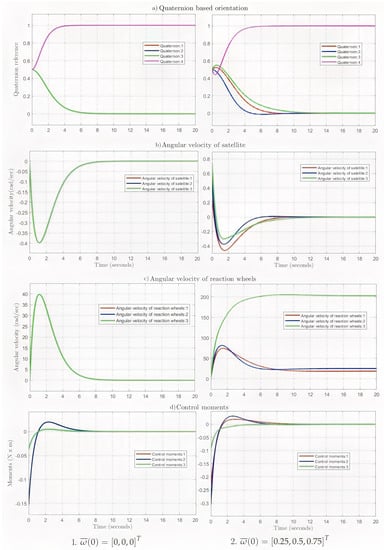
Figure 1.
Transient process calculation results.
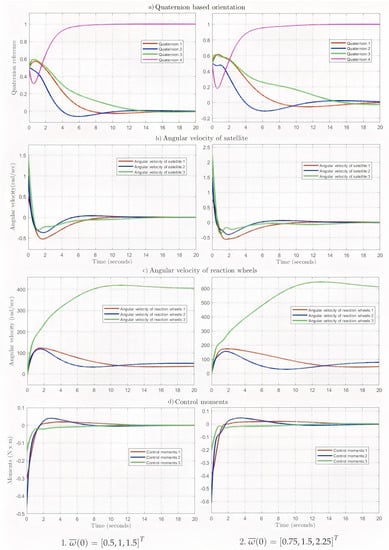
Figure 2.
Transient process calculation results.
The analysis of the numerical results obtained for the calculation of the transient processes in the SACS (Figure 1 and Figure 2) fully confirms the conclusions drawn from the qualitative analysis of the location of the roots of the normalized characteristic equation (Table 1).
At zero initial value for the angular momentum rad/s, the normalized (relative) transient process time was 8 s (Figure 1—1a). The transient process was aperiodic, with the maximum angular velocities of the satellite and reaction wheels equaling rad/s and 40 rad/s, respectively (Figure 1—1b,c). The maximum control moment created by the reaction wheels was N·m (Figure 1—1d).
At the initial value of the angular momentum corresponding to rad/s, the normalized (relative) transient time was 11 s (Figure 1—2a), the transient process had an oscillatory character, and the maximum angular velocities of the satellite and reaction wheels were rad/s and 210 rad/s, respectively (Figure 1—2b,c). The maximum control moment created by the reaction wheels was 0.3 N·m (Figure 1—2d).
At the initial value for the angular momentum corresponding to rad/s, the normalized (relative) transient time was 16 s (Figure 2—1a), the transient process had oscillatory characteristics, and the maximum angular velocities of the satellite and reaction wheels were equal 1.5 rad/s and 420 rad/s, respectively (Figure 2—1b,c). The maximum control moment created by the reaction wheels was equal to 0.45 N·m (Figure 2—1d).
At the maximum initial value for the angular momentum corresponding to rad/s, the normalized transient process time was 20 s (Figure 2—2a). The transient process was oscillatory, with the maximum angular velocities of the satellite and reaction wheels equaling 2.2 rad/s and 650 rad/s, respectively (Figure 2—2b,c). The maximum control moment created by the reaction wheels was 0.6 N·m (Figure 2—2d).
If the maximum angular velocities of the reaction wheels cannot be achieved with the available motors, then this means that the real transient process time must be longer than the normalized time. The real time value can be determined, as described in the authors’ work [18], by transitioning from normalized time to real time , the scale of which is determined as the ratio of the maximum angular velocity of the actual reaction wheel motor to the required maximum angular velocity for the normalized time.
9. Conclusions
- We described a mathematical model of the SACS, incorporating the equations of rotational dynamics and kinematics as well as the control law equations with a PD controller. The model is represented by a system of nonlinear differential equations. Based on the physical meaning of the state variables, it has been shown that the system of nonlinear differential equations satisfies all the conditions of Cauchy’s theorem about the existence and uniqueness of its solution when the initial conditions are set by the state variables. Given the existence and uniqueness of the solution to the system of nonlinear differential equations, it is proven that the angular velocities of the satellite and reaction wheels are continuous functions of time. From this, it follows that the satellite’s angular momentum, defined as a linear function of the satellite’s angular velocities, is a continuous function of time. Such an understanding of the satellite’s angular momentum as a physical quantity allows us to transform the nonlinear SACS model into a linear one.
- The asymptotic properties of the satellite’s angular momentum were investigated, and it was proven that in an asymptotically stable system, the angular momentum of the satellite relative to the associated coordinate system is represented by a sum of two components: a constant component, which is equal to its initial value in the inertial coordinate system, and a variable component, which asymptotically approaches zero as the rotation angles of the body frame relative to the inertial frame tend toward zero.
- Based on the analysis of the asymptotic properties of the satellite’s angular momentum, the nonlinear system of differential equations of the SACS’s rotational dynamics is represented by a linear system of differential equations which has time-variable but not constant parameters. This result allows the use of an exact linear model for the analysis of SACS dynamics instead of an approximate linearized model.
- We obtained the conditions for the asymptotic stability of the solution of the linear system of differential equations with time-variable parameters describing the rotational motion of the SACS. It was proven that the stability conditions of the obtained linear system of differential equations with time-variable parameters are determined by the conditions for the asymptotic stability of the solution of the linear system of differential equations with constant parameters. This result allows for the application of a rich arsenal of effective and practically tested engineering methods of analysis and the synthesis of linear automatic control systems when calculating and adjusting the SACS’s parameters.
- We investigated the influence of the control law parameters and the initial value of the satellite’s angular momentum on the indicators of stability and quality of transient processes in the SACS. It was shown that with an initial value of zero for the satellite’s angular momentum, the indicators of stability and quality of transient processes in the SACS depend only on the control law parameters. With an increase in the initial value of the satellite’s angular momentum, the indicators of stability and quality of transient processes deteriorate; the degree of stability decreases, the oscillation index worsens, and the transient process time increases. The use of these dependencies allows engineers to predict the range of changes in the dynamic characteristics of the SACS at the stage of initial satellite design.
- The statement about the global asymptotic stability of the SACS was proven in the case where the parameters of the control law were determined without taking into account the initial values of the angular momentum of the satellite. The statement is valid, provided that the roots of the characteristic equation of a truncated linear system with constant parameters are multiple, real, and negative, which corresponds to the requirement of maximum stability and maximum responsiveness for the SACS. The use of this statement will allow engineers to tune the parameters of the control law in the area of the most probable initial values of the satellite’s angular momentum.
- The results for the synthesis of control law parameters and the numerical solution of the SACS dynamics equations at different initial values for the satellite’s angular momentum were presented. These results confirm the previous theoretical conclusions made in this article.
Author Contributions
Conceptualization, M.M.; Methodology, M.M.; Validation, A.S.; Formal analysis, A.S.; Investigation, Y.O. and A.A.; Resources, Y.O. and A.A.; Data curation, Y.O. and A.A.; Writing—original draft, Y.O. and A.A.; Writing—review & editing, M.M.; Visualization, Y.O. and A.A.; Supervision, M.M. All authors have read and agreed to the published version of the manuscript.
Funding
This research has been funded by the Science Committee of the Ministry of Science and Higher Education of the Republic of Kazakhstan (Grant No. AP14869120).
Data Availability Statement
Not applicable.
Acknowledgments
The authors would like to thank the reviewers of the journal Mathematics for their valuable comments and advice on the first version of this article.
Conflicts of Interest
The authors declare no conflict of interest.
References
- Psiaki, M.L. Magnetic torquer attitude control via asymptotic periodic linear quadratic regulation. J. Guid. Control. Dyn. 2001, 24. [Google Scholar] [CrossRef]
- Doruk, R.O. Linearization in satellite attitude control with modified Rodriguez parameters. Aircr. Eng. Aerosp. Technol. Int. J. 2009, 81, 199–203. [Google Scholar] [CrossRef]
- Blanke, M.; Larsen, M.B. Satellite Dynamics and Control in a Quaternion Formulation, 2nd ed.; Department of Electrical Engineering, Technical University of Denmark: Lyngby, Denmark, 2010; 50p, Available online: https://orbit.dtu.dk/en/publications/satellite-dynamics-and-control-in-a-quaternion-formulation-2nd-ed (accessed on 28 May 2023).
- Rossa, F.D.; Dercole, F.; Lovera, M. Attitude stability analysis for an Earth pointing, magnetically controlled spacecraft. IFAC Proc. Vol. 2013, 46, 518–523. Available online: https://www.researchgate.net/publication/288549058_Attitude_stability_analysis_for_an_Earth_pointing_magnetically_controlled_spacecraft (accessed on 28 May 2023). [CrossRef]
- Mehrjardi, M.F.; Sanusi, H.; Ali, M.A.M.; Taher, M.A. PD Controller for three-axis satellite attitude control using discrete Kalman filter. In Proceedings of the 2014 International Conference on Computer, Communications, and Control Technology (I4CT), Langkawi, Malaysia, 2–4 September 2014. [Google Scholar] [CrossRef]
- Ran, D.; Sheng, T.; Cao, L.; Chen, X.; Zhao, Y. Attitude control system design and on-orbit performance analysis of nano-satellite Tian Tuo 1. Chin. J. Aeronaut. 2014, 27, 593–601. [Google Scholar] [CrossRef]
- Zhou, B. On Stability of the Linearized Spacecraft Attitude Control System. 2015. Available online: https://arxiv.org/pdf/1504.00114.pdf (accessed on 14 April 2023).
- Moldabekov, M.; Yelubayev, S.; Alipbayev, K.; Sukhenko, A.; Bopeyev, T.; Mikhailenko, D. Stability analysis of the microsatellite attitude control system. Appl. Mech. Mater. 2015, 798, 297–302. [Google Scholar] [CrossRef]
- Galvao, B.B.; Faustino, M.C.M.; de Souza, L.C.G. Satellite attitude control system design with nonlinear dynamics and kinematics of quaternion using reaction wheels. In Proceedings of the XXXVII Iberian Latin-American Congress on Computational Methods in Engineering, Brasília, Brazil, 6–9 November 2016. [Google Scholar] [CrossRef]
- Nasrolahi, S.S.; Abdollahi, F. Lyapunov stability analysis for non-linear satellite attitude control in the presence of states measurement error. In Proceedings of the 4th International Conference on Control, Instrumentation and Automation, Qazvin, Iran, 27–28 January 2016. [Google Scholar] [CrossRef]
- Moldabekov, M.; Akhmedov, D.; Yelubaev, S.; Alipbayev, K.; Sukhenko, A. Optimal synthesis of satellite orientation system’s parameters. Adv. Astronaut. Sci. 2017, 161, 989–997. Available online: http://www.univelt.com/book=6305 (accessed on 14 April 2023).
- Ocampo, C. Modeling, simulation, and control of the spacecraft attitude dynamics. Cuad. Ing. MatemáTica 2019, 101. [Google Scholar] [CrossRef]
- Narkiewicz, J.; Sochacki, M.; Zakrzewski, B. Generic Model of a Satellite Attitude Control System. Int. J. Aerosp. Eng. 2020, 2020, 5352019. [Google Scholar] [CrossRef]
- Demidovich, B.P. Lectures on Mathematical Theory of Stability (Lekcii po Matematicheskoi Teorii Ustoichivosti). Nauka, Moscow. 1967. 472p. Available online: https://ikfia.ysn.ru/wp-content/uploads/2018/01/Demidovich1967ru.pdf (accessed on 14 April 2023). (In Russian).
- Okasha, M.; Idres, M.; Ghaffar, A. Satellite Attitude Tracking Control Using Lyapunov Control Theory. Int. J. Recent Technol. Eng. (IJRTE) 2019, 7, 253–257, ISSN 2277-3878. Available online: https://www.ijrte.org/wp-content/uploads/papers/v7i6s/F02490376S19.pdf (accessed on 14 April 2023).
- Navabi, M.; Hosseini, M.R. Spacecraft Quaternion Based Attitude Input-Output Feedback Linearization Control Using Reaction Wheels. In Proceedings of the 2017 8th International Conference on Recent Advances in Space Technologies (RAST), Istanbul, Turkey, 19–22 June 2017; Available online: https://doi.org/10.1109/RAST.2017.8002994 (accessed on 14 April 2023).
- Romero, A.G.; Souza, L.C. Satellite Controller System Based on Reaction Wheels Using the State-Dependent Riccati Equation (SDRE) on Java. In Proceedings of the 10th International Conference on Rotor Dynamics—IFToMM; IFToMM 2018; Cavalca, K., Weber, H., Eds.; Springer: Cham, Switzerland, 2019; Volume 61, pp. 547–561. Available online: https://doi.org/10.1007/978-3-319-99268-6_38 (accessed on 14 April 2023).
- Moldabekov, M.; Sukhenko, A.; Shapovalova, D.; Yelubayev, S. Using the linear form of equations of dynamics of satellite attitude control system for its analysis and synthesis. J. Theor. Appl. Mech. 2020, 59, 109–120. [Google Scholar] [CrossRef] [PubMed]
- Knudsen, J.M.; Hjorth, P.G. Elements of Newtonian Mechanics, 1st ed.; Springer: Berlin, Germany, 1995; Available online: https://www.abebooks.com/servlet/BookDetailsPL?bi=14875248608&searchurl=an%3Dknudsen%2Bhjorth%26sortby%3D17&cm_sp=snippet-_-srp1-_-title1 (accessed on 14 April 2023).
- Markeev, A.P. Theoretical Mechanics: A Textbook for Universities; CheRo: Moscow, Russia, 1999; 572p, Available online: http://pm-pu.ru/stuff/adus/books/markeev_tm.pdf (accessed on 14 April 2023). (In Russian)
- Sidi, M. Spacecraft Dynamics and Control: A Practical Engineering Approach (Cambridge Aerospace Series); Cambridge University Press: Cambridge, UK, 1997. [Google Scholar] [CrossRef]
- Wie, B.; Lu, J. Feedback control logic for spacecraft eigenaxis rotations under slew rate and control constraints. J. Guid. Control Dyn. 1995, 18, 1372–1379. [Google Scholar] [CrossRef]
- Wirkus, A.S.; Swift, J.R. A Course in Ordinary Differential Equations, 2nd ed.; Chapman and Hall/CRC: Boca Raton, FL, USA, 2014. [Google Scholar] [CrossRef]
- Zwillinger, D. Handbook of Differential Equations, 3rd ed.; Academic Press: Boston, MA, USA, 1997. [Google Scholar]
- Chaurais, J.R.; Ferreira, H.C.; Ishihara, J.I.; Borges, R.A.; Kulabukhov, A.M.; Larin, V.A.; Belikov, V.V. A high precision attitude determination and control system for the UYS-1 nanosatellite. In Proceedings of the IEEE Aerospace Conference, Big Sky, MT, USA, 2–9 March 2013. [Google Scholar] [CrossRef]


Disclaimer/Publisher’s Note: The statements, opinions and data contained in all publications are solely those of the individual author(s) and contributor(s) and not of MDPI and/or the editor(s). MDPI and/or the editor(s) disclaim responsibility for any injury to people or property resulting from any ideas, methods, instructions or products referred to in the content. |
© 2023 by the authors. Licensee MDPI, Basel, Switzerland. This article is an open access article distributed under the terms and conditions of the Creative Commons Attribution (CC BY) license (https://creativecommons.org/licenses/by/4.0/).