

Attractors in Pattern Iterations of Flat Top Tent Maps

CIMA and Department of Mathematics of ISEL-Higher Institute of Engineering of Lisbon, Rua Conselheiro Emídio Navarro, 1, 1959-007 Lisbon, Portugal
Mathematics 2023, 11(12), 2677; https://doi.org/10.3390/math11122677
Submission received: 10 May 2023
/
Revised: 7 June 2023
/
Accepted: 11 June 2023
/
Published: 13 June 2023
(This article belongs to the Special Issue Applied Mathematical Modelling and Dynamical Systems)
Abstract
:Flat-topped one-dimensional maps have been used in the control of chaos in one-dimensional dynamical systems. In these applications, this mechanism is known as simple limiter control. In this paper, we will consider the introduction of simple limiters u in the tent map, according to a time-dependent scheme defined by a binary sequence s, the iteration pattern. We will define local and Milnor attractors in this non-autonomous context and study the dependence of their existence and coexistence on the value of the limiter u and on the pattern s. Using symbolic dynamics, we will be able to characterize the families of pairs for which these attractors exist and coexist, as well as fully describe them. We will observe that this non-autonomous context provides a richness of behaviors that are not possible in the autonomous case.
MSC:
37E05; 37B55; 37G35; 37B101. Introduction
In recent years, the study of piecewise smooth maps has attracted the attention of several authors (see [1] and references therein). This, in part, is due to the fact that many real-world processes, characterized by sharp switching between the states, are naturally represented by this kind of map. A particular class of piecewise smooth maps are the flat-topped maps, which are obtained through the insertion of a flat segment on a one-dimensional map. This procedure, known as simple limiter control, often leads to a superstable periodic orbit and has been widely used in the control of chaos on one-dimensional dynamical systems [2,3,4,5,6], which is applicable in areas as diverse as cardiac dynamics [7,8], telecommunications or electronic circuits [6,9], population dynamics [10], or dynamics of commodity markets [11].
Very often, we find modeling situations wherein evolutionary equations have to depend explicitly on time, through time-dependent parameters. This is the case, for example, when we want to model populations with time-dependent forcing or to mimic some control or regulation strategies. Based on this premise, some recent studies have looked at how the traditional theory extends when alternating two different real [12,13,14] or complex maps [15,16] in the iteration.
In these situations, we get into the field of non-autonomous dynamical systems, that, in this work, will be restricted to systems generated by non-autonomous difference equations of the type
where is a one-parameter family of one-dimensional maps and is a sequence of parameters.
In [11], the authors developed a behavioral commodity market model with the imposition of price limiters, bottoming or topping price levels, and discussed how the on–off switching of this stabilization mechanism as well as changing the level of price limiters may interfere with the price discovery process.
In [17], the iteration scheme was considered for the complex logistic family , , , and how the sequence can affect the topology of the Julia and Mandelbrot sets was studied. For a fixed pair of parameters , the sequence is identified by a binary sequence , the iteration pattern.
In this paper, we will consider a class of non-autonomous dynamical systems generated by an analogous iteration scheme, for a family of flat top tent maps with a segment with constant value u, considering an iteration pattern , such that the zero positions in s correspond to iterating the function and the one positions correspond to iterating the tent map T (the instants corresponding to an index 0 in s are those at which a limiter is introduced). We will focus on the existence of attractors (invariant and attracting sets) and their dependence on the parameter u and on the iteration pattern s.
Beyond the creation of superstable periodic orbits, it was observed in [18] that the insertion of a flat segment on a one-dimensional map may lead to a situation wherein the constant interval is mapped to a point of an unstable periodic orbit of T, and so this unstable orbit attracts a set of points of positive Lebesgue measure. Invariant sets of this kind are commonly known as Milnor attractors.
The dynamics of non-autonomous dynamical systems depends, in addition to the initial value, on the initial instant. This simple fact, compared with the autonomous case, results in relevant changes in the concept of attractor, which were addressed in [19,20].
We will define local attractors and Milnor attractors in the context of the non-autonomous systems that we intend to study and discuss how they depend on the pair . Following [19,20], these attractors are invariant and attractive subsets (non-autonomous sets). Using symbolic dynamics, we will obtain natural classes of pairs that generate such attractors, as well as fully describe them.
Unlike autonomous unimodal systems with one flat segment, where only one attractor can exist at a time, we will observe that, in the non-autonomous case, several attractors can coexist simultaneously, thus showing the richness of behaviors in the non-autonomous case. We will establish the conditions on the pairs for which there is a coexistence of attractors.
A non-autonomous dynamical system of type (1) is periodic if is a periodic sequence. Many of the properties of the non-autonomous p-periodic systems may be deduced from the properties of the p autonomous systems , . Taking this observation into account, we emphasize that our results do not require the periodicity of , which, in our case, is translated by the periodicity of the iteration pattern s.
In Section 2, we will define the pattern iteration of flat top tent maps and introduce symbolic dynamics for these systems. In Section 3, we will introduce non-autonomous local attractors and non-autonomous Milnor attractors and study their existence and coexistence, depending on the parameters . Finally, in Section 4, we summarize the main conclusions of this paper and discuss possible applications and generalizations.
2. Pattern Iterations of Flat Top Tent Maps
We study sequential iterations of two different maps, and , according to a general binary sequence (iteration pattern), in which:
- The “zero” positions correspond to iterating the function ;
- The “one” positions correspond to iterating the function .
The maps belong to the family of flat top tent maps , , such that
Note that the interval is used both for the parameters space and the phase space.
The extended parameters space is
Through this paper, we fixate , so is the usual tent map
The notation , represents the concatenation of n copies of the finite sequence . If , then it represents a p-periodic infinite sequence.
If , then the sequential iteration is simply the iteration of the tent map, and if , it is the iteration of .
In the non-autonomous context, the dynamics depend, in addition to the initial value, on the starting time. To address this, we will make use of the extended state space
For , and , define the n-th iteration on x with initial time k as
Define the symbolic address of a point , as
Definition 1.
For and define the orbit of x with initial time k as the sequence
and the itinerary of as the symbolic sequence
Definition 2.
For , define the itinerary of x under the tent map as the symbolic sequence
The itineraries of pattern iterations lie in the set of infinite sequences such that for all . On the other hand, since , then the orbit of 0 under T becomes trapped in the fixed point , so the itineraries under T will be contained in the subset of all infinite sequences such that if for some i, then .
Considering the natural order , we will now introduce an order structure in .
Define
For and , let
Now, for , if and only if or there exists , such that for all and .
Let , be the shift map.
Definition 3.
A sequence is maximal if for all .
The following is a classic result in symbolic dynamics, and its proof can be found, for example, in [21].
Lemma 1.
For any , if and only if .
Consider the map , such that and, for all ,
where n is such that and if for all .
In [22], we proved the following.
Theorem 1.
For all , and .
3. Non-Autonomous Attractors
In the non-autonomous context, attractors and repellers live naturally in the extended state space. To address this, in [19], Potzsche discussed these concepts based on the idea of non-autonomous set, defined below:
Definition 4.
A non-autonomous set is a subset of the extended state space .
Definition 5.
Let be a non-autonomous set, then:
- The k-fiber of is
- The fiber projection of is
- is projection closed ifis closed.
- is p-cyclic if there exists k such that for all , .
Definition 6.
Let be a non-autonomous set and , then:
- is invariant if there exists k such that for all , .
- is locally attractive if it is invariant and there exists l such that for each , there exists a neighborhood of in such that for some n.
Definition 7.
Let be a non-autonomous set and . Then, is a local attractor if it is projection closed, locally attractive and there is not any non-autonomous set with that satisfies these properties.
For a sequence , if for all n and is p-periodic, then the set of the terms of is the projection of an local attractor. However, local attractors are not the only kind of attractors. Indeed, if u is mapped after some iteration steps into a point of an unstable periodic orbit, then this orbit will attract a set of positive Lebesgue measures, but will possibly not attract any neighborhood of itself. These orbits were designated in [18] as Milnor attractors.
In [23], in the autonomous context, Milnor discussed the idea of attractor in a weaker sense, namely as a closed invariant set such that its stable set has a positive measure and there is no smaller subset such that coincides with except for a set of measure zero, see [18].
In the following definition, we adapt this concept to the non-autonomous context.
For each and , let and, for each non-autonomous set ,
Let be the Lebesgue measure in .
Definition 8.
For , a Milnor attractor is a projection closed invariant non-autonomous set for which there is such that, for all , and there is not any non-autonomous set with that satisfies the same properties.
Remark 1.
We will refer to the last condition in both Definitions 7 and 8, “there is not any non-autonomous set with that satisfies the same properties”, with being projection minimal.
Remark 2.
An local attractor is a Milnor attractor but the opposite is not necessarily true.
3.1. The Case Maximal
We will first study the case wherein is a maximal sequence. From Lemma 1, this implies that for all i such that , so for any i, and . This means that if is maximal, then in the entire orbit set , it makes no difference to apply or T.
For an iteration pattern , let
Let be a p-periodic sequence, and be the non-autonomous set such that for all ().
Theorem 2
(Existence of Milnor attractors). Let be a p-periodic sequence and be such that:
- 1.
- .
- 2.
- is maximal.
- 3.
- .
Then, is a Milnor attractor.
Proof.
Since X is periodic, then is projection-closed.
From Condition 1 , so from Condition 2 and Theorem 1, for all
and is -invariant. From its definition, no other non-autonomous set such that could be invariant so is projection-minimal.
For any , let , exists from Condition 3. Then, from Condition 2, for all
so and, since , then has positive measure. □
Remark 3.
In [20] is introduced a notion of finite-time attractivity, mainly focused in the speed of convergence. It warrants that some kind of convergence happens in finite time. In the present context, the convergence always happens in finite time, for each m.
Theorem 3
(Existence of local attractors). Let be such that:
- 1.
- There is p minimal such that .
- 2.
- is maximal.
- 3.
- There is j such that for all .
Then, the non-autonomous set such that if and for all is an local attractor if and only if . Moreover, this local attractor is p-cyclic.
Proof.
Since , is projection-closed. Since U is maximal, for all , so is invariant and this implies that it is also projection-minimal.
Now, we will see that is locally attractive if and only if .
U maximal and p-periodic implies that is a pre-image of u under T, so .
We will make the proof only considering , since it follows analogously for . We will also suppose without loss of generality that and consequently for all n.
Suppose first that . If then for all .
Since then , so and is decreasing and onto in a neighborhood of u, so in this neighborhood there is such that . Analogously, in this neighborhood there is such that . Consider now the neighborhood of , , and . On the one hand, since U is maximal, then
and, because ,
On the other hand, , so and . We conclude that is attracting. The cyclicity of is immediate from the definition.
If , then since , is increasing in a neighborhood of u, so for any n, if is close enough to u, then and . □
It follows from the definitions that, for pattern iterations of flat top tent maps, any local attractor or Milnor attractor must attract and consequently u. Since if U is maximal then the iterates do not depend on the starting time k, we can conclude the following.
Theorem 4.
If is maximal then, for any , there can not exist two attractors and , local or Milnor, with different fiber projections .
3.2. The Case Non-Maximal
Let us now study what happens when is not maximal. In this context, we must consider defined in the following way:
Let be such that , then
Theorem 5
(Existence of Milnor attractors). Let be a p-periodic sequence and be such that is not maximal and
- 1.
- For all , .
- 2.
- .
- 3.
- .
Then is an Milnor attractor.
Proof.
Condition 1 allows us to use the same arguments as in Theorem 2 to conclude that is invariant and projection-minimal.
For any , let , exists due to condition 3. Now, let be the left branch of the tent map,
and
For we have that and for all j. Moreover, for , we have that, for all j, , so for all , and, since then , so and . □
Remark 4.
Conditions 1 and 2 in the previous Theorem imply that for all i.
Remark 5.
Note that Milnor attractors, on one hand, are not robust in relation with the parameter u, in the sense that the attractor does not persist under small perturbations of u, but on the other hand they present a certain robustness in relation with the iteration pattern s. From Theorem 2, if is maximal then the attractor persists for all patterns s such that and, from Theorem 5, if is not maximal then the attractor persists for all patterns s such that .
Consider now , then is not maximal because , so implies that and there is such that and . Let be such that ; then, for all , and we have that, if s is such that for all n, then the non-autonomous set such that and for all is a local attractor. Therefore, the introduction of the condition for all n created a 2-cyclic local attractor, see Figure 1.
More generally, if U is such that for some k, let
then we have the following Theorem.
Theorem 6
(Existence of local attractors). Let be such that:
- 1.
- is not maximal, i.e., there exists k such that .
- 2.
- There is such that, for all and , and .
Then, the non-autonomous set such that for all and, for all , and , , is a k-cyclic local attractor.
Proof.
We will consider . If , then, from Lemma 1 . On the other hand, for all implies that and so . Moreover, for all
and
so is invariant and k-cyclic and so it is also projection-minimal. On the other hand, since, for all n, is onto in each of its branches of monotonicity, there are such that is monotonous and . For each and each we consider the neighborhoods of , . To simplify the notation, we will consider .
If there is no such that and , then
On the other hand, if there is such that and then, from Condition (2) and the monotonicity of , we have that
or
for some .
Without loss of generality, we will only consider the first situation.
Then,
Suppose that i is unique, then
If i is not unique, i.e., if there is
such that, for all , and , then, as before, we can take such that
so
If we continue this procedure, then
Just as for we can consider such that
and
Therefore, we conclude that
and, recursively, that
Finally, we have
□
Example 1.
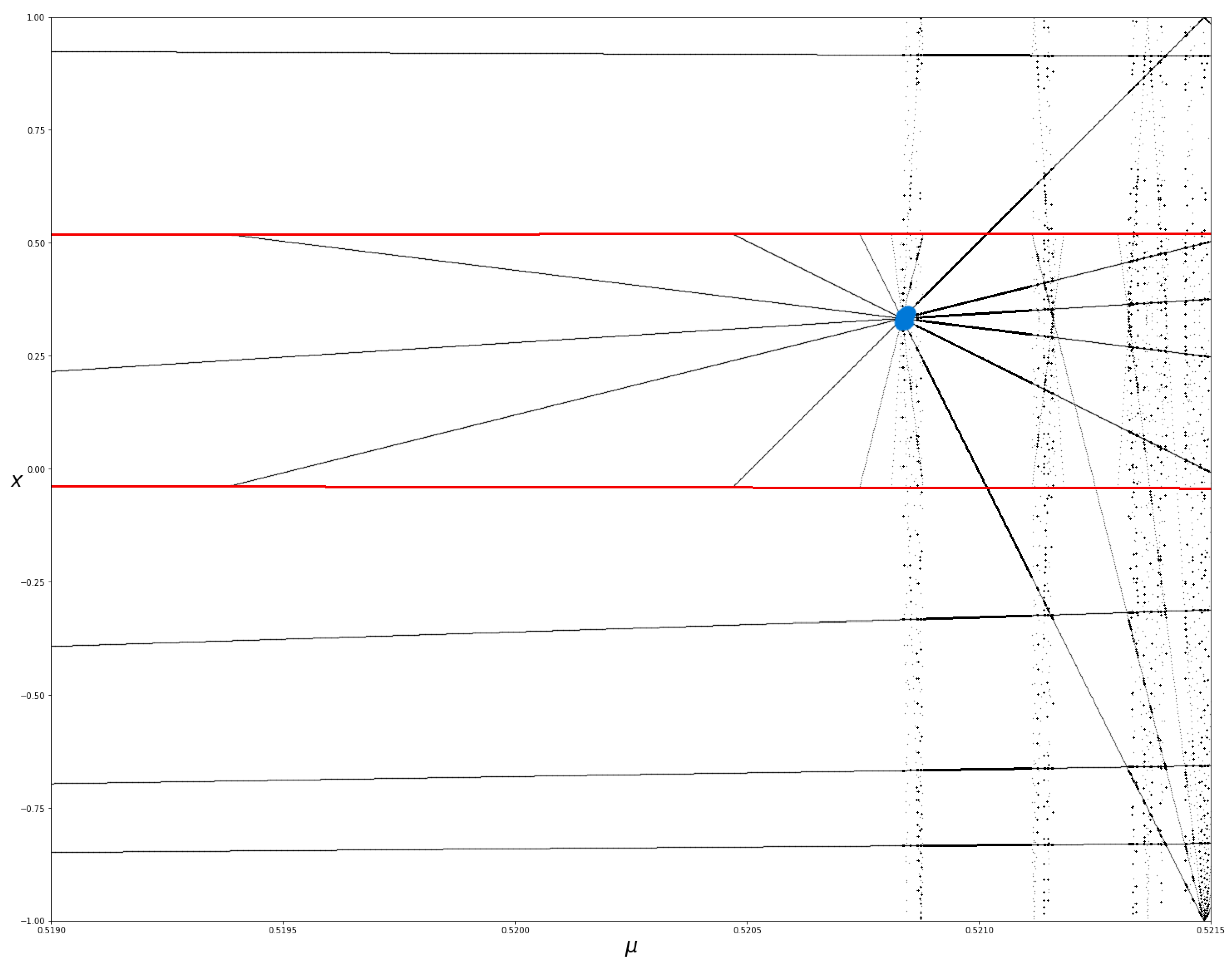
Let us consider the iteration pattern , and . We have that and , so, from Lemma 1, for any parameter , and, since , and for all , from Theorem 6 the system has a 2-cyclic local attractor. This can be seen in Figure 2, where the attractor is depicted in red.
Looking now at the point depicted in blue in Figure 2, it has coordinates and
Numerically, is a fixed point of T.
Having in mind Theorem 5, for , , so . On the other hand, for all , and , therefore . Therefore, considering , is a Milnor attractor. We conclude that, for and one local attractor and one Milnor attractor coexist. Note that this is just possible because is not maximal.
We can merge Theorems 5 and 6 to obtain the following.
Theorem 7
(Coexistence of local attractors and Milnor attractors). Let be a p-periodic sequence and be such that:
- 1.
- For all , .
- 2.
- such that .
- 3.
- For there is l such that .
- 4.
- .
- 5.
- There is an order such that, for all , and for all .
Then, the non-autonomous set such that for all and , for is an local attractor and is a Milnor attractor.
We will see in the following example that, in the non-maximal case two local attractors can also coexist.
Example 2.
Consider again, and, now, . We have that
It is easy to verify that and are the only such that , so, regarding Theorem 6, . Since s is 6-periodic, and , then and for all , so, from Theorem 6, the non-autonomous set such that for all and all is a 12-cyclic local attractor. Since , this 12-cyclic local attractor coexists with the 2-cyclic one studied in Example 1. Looking at Figure 2, we see that this situation persists in a neighborhood around .
There is another remarkable difference between the maximal and non-maximal cases: From Theorem 3, in the maximal case all local attractors are cyclic. To illustrate the non-maximal case consider now and . Evidently, U is not maximal because and . Now, adapting the arguments of the proof of Theorem 6, for any iteration pattern , where , the non-autonomous set such that and for all is an local attractor but, in spite of
unlike in the maximal case, it may be non-cyclic. This is the case when the sequence is neither periodic nor eventually periodic.
In this case, we may still have coexistence of a local attractor with an Milnor attractor. Consider for example a pattern
such that, for all i, and .
On one hand, we have a subsequence such that, for all j, and and this generates the local attractor. On the other hand, we have an infinite subsequence such that, for all j, and and this generates the Milnor attractor.
Remark 6.
A more general formulation for sufficient conditions for the existence of an local attractor is the existence of such that for all and one sequence such that, for all , and there exists such that and for all .
4. Discussion and Conclusions
It was previously known that the introduction of simple limiters in one-dimensional maps may create superstable periodic orbits as well as Milnor attractors. With this paper, we have provided evidence that supports the conclusion that, to create these attractors, it is not necessary to introduce the limiter in all iteration steps, not even periodically. Moreover, the non-autonomous systems studied exhibit a richness of different behaviors that could not be observed in the unimodal autonomous case. Unlike the autonomous case, where each limiter u can only lead to the creation of one attractor and wherein it is required for the local attractors to be cyclic, in the non-autonomous case, depending on the chosen pattern, each limiter u may lead to the creation of multiple attractors. Furthermore, in the non-autonomous case, it is possible for there to be non-cyclic local attractors and for several attractors, of the same or different types, to coexist.
In [10], it is stated that, in biological terms, the application of a simple limiter to the one-dimensional map corresponds to control measures such as culling of a stock population, hunting or catching of a managed population and stock. However, they show that applying limiter control to a state variable can significantly shift its mean value, making this measure counter-effective in many situations.
Similarly, in [11] it is observed that the introduction of low limiters in the prices may lower the average price and the introduction of upper limiters may increase it. It is also stated that price limiter policies may lead to substantial costs for the central authority. For example, to prevent the price from dropping below (going above) the minimum (maximum) price, the central authority has to permanently buy (sell) a fraction of the supplied (stored) commodity. Therefore, it is reasonable to presume that, by reducing the number of times the limiters are introduced, we may be able to bring down the implementation costs.
In order to further test this assumption, it would be of interest to apply our methods to the models of [10,11] in an attempt to control the average values and reduce the implementation costs.
In the context of this article, the parameter u defines the limiter and the iteration pattern s defines the strategy of implementation of the limiter. For example, considering the introduction of a limiter , we obtain the same 2-cyclic local attractor with , regardless of whether the limiter is applied permanently () 0r alternately (), which could translate into a potential reduction in the costs. On the other hand, for we will have a local 12-periodic attractor with a different mean value of its orbits and an even longer time delay between the application of limiters.
Throughout this article, a periodicity condition was never imposed on the iteration pattern s, which allows us to consider that this is located in the field of non-autonomous non-periodic dynamical systems.
Although exclusively tent maps were considered, the results achieved can easily be generalized to other unimodal maps, such as the quadratic map , for example.
If we drop the restriction , considering two flat top tent maps with will provide additional complexity, including the coexistence of attractors related to both plateaus, codimension two bifurcations such as those studied in [13], complicated symbolic Dynamics, etc. Lastly, it is expected that this generalization is very similar to the generalization to l-modal piecewise linear maps with plateaus.
Funding
This work was partially supported by FCT Fundação para a Ciência e a Tecnologia, Portugal, through the project UID/MAT/04674/2013, CIMA and ISEL.
Data Availability Statement
Not applicable.
Conflicts of Interest
The author declares no conflict of interest.
References
- Avrutin, V.; Gardini, L.; Sushko, I.; Tramontana, F. Continuous and Discontinuous Piecewise-Smooth One-Dimensional Maps: Invariant Sets and Bifurcation Structures; World Scientific Series on Nonlinear Science; World Scientific: Singapore, 2019; Volume 95. [Google Scholar]
- Corron, N.J.; Pethel, S.D.; Hopper, B.A. Controlling Chaos with Simple Limiters. Phys. Rev. Lett. 2000, 84, 3835–3838. [Google Scholar] [CrossRef] [PubMed]
- Myneni, K.; Barr, T.A.; Corron, N.J.; Pethel, S.D. New method for the control of fast chaotic oscillations. Phys. Rev. Lett. 1999, 83, 2175–2178. [Google Scholar] [CrossRef]
- Stoop, R.; Wagner, C. Scaling Properties of Simple Limiter Control. Phys. Rev. Lett. 2003, 90, 154101–154104. [Google Scholar] [CrossRef] [PubMed] [Green Version]
- Wagner, C.; Stoop, R. Optimized chaos control with simple limiters. Phys. Rev. E 2000, 63, 17201–17202. [Google Scholar] [CrossRef] [PubMed] [Green Version]
- Wagner, C.; Stoop, R. Renormalization Approach to Optimal Limiter Control in 1-D Chaotic Systems. J. Stat. Phys. 2002, 106, 97–106. [Google Scholar] [CrossRef]
- Garfinkel, A.; Spano, M.; Ditto, W.; Weiss, J. Controlling cardiac chaos. Science 1992, 84, 1230–1235. [Google Scholar] [CrossRef] [PubMed] [Green Version]
- Glass, L.; Zeng, W. Bifurcations in flat-topped maps and the control of cardiac chaos. Int. J. Bifurc. Chaos 1994, 4, 1061–1067. [Google Scholar] [CrossRef]
- Matsuoka, Y.; Saito, T. Rotation Map with a Controlling Segment and Its Application to A/D Converters. IEICI Trans. Fundam. 2008, E91-A, 1725–1732. [Google Scholar] [CrossRef] [Green Version]
- Westeroff, F.M.H.A.H. Paradox of simple limiter control. Phys. Rev. E 2006, 73, 052901. [Google Scholar]
- He, X.-Z.; Westerhoff, F.H. Commodity markets, price limiters and speculative price dynamics. J. Econ. Dyn. Control 2005, 29, 1577–1596. [Google Scholar] [CrossRef] [Green Version]
- Rădulescu, A. The connected isentropes conjecture in a space of quartic polynomials. Discret. Contin. Dyn. Syst. 2007, 19, 139–175. [Google Scholar] [CrossRef]
- Silva, L.; Rocha, J.L.; Silva, M.T. Bifurcations of 2-periodic non-autonomous stunted tent systems. Int. J. Bifurcation Chaos 2017, 27, 1730020–1730037. [Google Scholar] [CrossRef]
- Silva, M.T.; Silva, L.; Fernandes, S. Convergence rates for sequences of bifurcation parameters of non-autonomous dynamical systems generated by flat top tent maps. Commun. Nonlinear Sci. Numer. Simul. 2020, 81, 105007. [Google Scholar] [CrossRef]
- Danca, M.-F.; Bourke, P.; Romera, M. Graphical exploration of the connectivity sets of alternated julia sets. Nonlinear Dyn. 2013, 73, 1155–1163. [Google Scholar] [CrossRef] [Green Version]
- Danca, M.-F.; Romera, M.; Pastor, G. Alternated julia sets and connectivity properties. Int. J. Bifurc. Chaos 2009, 19, 2123–2129. [Google Scholar] [CrossRef] [Green Version]
- Rădulescu, A.; Pignatelli, A. Symbolic template iterations of complex quadratic maps. Nonlinear Dyn. 2016, 84, 2025–2042. [Google Scholar] [CrossRef] [Green Version]
- Avrutin, V.; Futter, B.; Gardini, L.; Schanz, M. Unstable orbits and Milnor attractors in the discontinuous flat top tent map. ESAIM Proc. 2012, 36, 126–158. [Google Scholar] [CrossRef]
- Pötzsche, C. Bifurcations in non-autonomous Dynamical Systems: Results and tools in discrete time. In Proceedings of the International Workshop Future Directions in Difference Equations; Liz, E., Mañosa, V., Eds.; Universidade de Vigo: Vigo, Spain, 2011; pp. 163–212. [Google Scholar]
- Rasmussen, M. Attractivity and Bifurcation for Non-Autonomous Dynamical Systems; Lect. Notes in Mathematics; Springer: Berlin/Heidelberg, Germany, 2007; Volume 1907. [Google Scholar]
- Collet, P. ; Eckmann, J-P. Iterated Maps on the Interval as Dynamical Systems; Birkhäuser: Boston, MA, USA, 2009. [Google Scholar]
- Silva, L. Periodic attractors of non-autonomous flat-topped tent systems. Discret. Contin. Dyn. Syst.-B 2018, 24, 1867–1874. [Google Scholar]
- Milnor, J.W. On the Concept of Attractor. Commun. Math. Phys. 1985, 99, 177–195. [Google Scholar] [CrossRef]
Figure 1.
Pattern iteration with . If , then the only iterate of order less than 6 that lies in is , so the only that can change the orbit are .
Figure 1.
Pattern iteration with . If , then the only iterate of order less than 6 that lies in is , so the only that can change the orbit are .

Figure 2.
Bifurcation diagram with and . We iterated 1500 times with initial value 0 and initial instant 0. The 2-cyclic local attractor is depicted in red and the Milnor attractor is the blue point. The black lines on the left side of the Milnor attractor correspond to transient regimes before the trajectories become trapped in the local attractor. On the right side of the Milnor attractor, the black lines may correspond to other local attractors coexisting with the 2-cyclic.
Disclaimer/Publisher’s Note: The statements, opinions and data contained in all publications are solely those of the individual author(s) and contributor(s) and not of MDPI and/or the editor(s). MDPI and/or the editor(s) disclaim responsibility for any injury to people or property resulting from any ideas, methods, instructions or products referred to in the content. |
© 2023 by the author. Licensee MDPI, Basel, Switzerland. This article is an open access article distributed under the terms and conditions of the Creative Commons Attribution (CC BY) license (https://creativecommons.org/licenses/by/4.0/).
Share and Cite
MDPI and ACS Style
Silva, L. Attractors in Pattern Iterations of Flat Top Tent Maps. Mathematics 2023, 11, 2677. https://doi.org/10.3390/math11122677
AMA Style
Silva L. Attractors in Pattern Iterations of Flat Top Tent Maps. Mathematics. 2023; 11(12):2677. https://doi.org/10.3390/math11122677
Chicago/Turabian StyleSilva, Luis. 2023. "Attractors in Pattern Iterations of Flat Top Tent Maps" Mathematics 11, no. 12: 2677. https://doi.org/10.3390/math11122677
Note that from the first issue of 2016, this journal uses article numbers instead of page numbers. See further details here.