The NBRULC Reliability Class: Mathematical Theory and Goodness-of-Fit Testing with Applications to Asymmetric Censored and Uncensored Data

Abstract

The majority of approaches proposed in the past few decades to solve life test problems have differed markedly from those used for closely related, yet broader, issues. Due to the complexity of data that are generated each day in many practical domains, as a result of the development of scales for rating the success or failure of reliability, a new domain of reliability has been created. This domain is referred to as life classes, where specific probability distributions are presented. In this study, it is shown that the use of the quality-of-fit technique to solve problems involving life testing makes sense, and produces simpler processes that are roughly equivalent or superior to those used in traditional procedures. They may also behave better in limited samples. This work investigates a novel quality-of-fit test statistic; it is based on an exponential transform and is compared to the best renewal used Laplace test in increasing convex ordering (NBRULC). Evidence for approach normality is provided. The calculated variables include powers, Pitman asymptotic effectiveness, and critical points. Methods on how to handle censored data were also studied. Our experiments have real-world applications in the fields of medicine and engineering.

1. Introduction

Reliability can be compared to quality over time. Since workmanship and manufacturing are quality factors, a product would be deemed as low quality if it malfunctions or breaks right after purchase. Poor reliability, on the other hand, is when product components fail before one anticipates them to. Therefore, there is a distinction between quality and reliability that has to do with time, more precisely, the product’s lifetime. Reliability is officially defined as the capacity of a thing to carry out an essential task under predetermined circumstances for a predetermined amount of time. The likelihood of an item performing a necessary function under specified conditions for a specific amount of time is another definition that addresses the probabilistic nature of assessing reliability. As a result, reliability is a measure of technical uncertainty, and estimating reliability requires the application of statistics, specifically the probability theory. Testing completed items or components under settings that mimic real-world use until failure occurs is the typical method for gauging system reliability. Although it may seem that having more data would increase one’s trust in the reliability level, this practice is frequently costly and time-consuming. Therefore, it is particularly important to consider the lifespan of products before all test units experience a malfunction. Aging concepts explain how a part or a system can experience improvements or deterioration as it ages. According to the aging characteristics, many types of life distributions are categorized or characterized in the literature. The exponential distribution almost always falls into one of these classifications, which is a significant feature in such classifications. Any reliability analysis must take stochastic aging into account, and numerous test statistics have been established in the literature, comparing exponential growth to various aging options. Our objective is to provide an overview of these advancements. Researchers in statistics and reliability analysis have looked at testing exponentiality problems using different age classes of life distributions from a variety of angles; for more information, see Bryson and Siddiqui [1], Bhattacharyya et al. [2], Barlow and Proschan [3], Klefsjo [4], Khan et al. [5], Kumazawa [6], Mahmoud et al. [7,8], Majumder and Mitra [9], Bhattacharyya et al. [10], Navarro [11], Abu-Youssef et al. [12], Ghosh and Mitra [13], Navarro and Pellerey [14], El-Morshedy et al. [15], EL-Sagheer et al. [16] Gadallah et al. [17], Mansour [18], Ghosh and Mitra [19], Majumder and Mitra [20], Lai and Xie [21], Etman et al. [22], Ghosh and Majumder [23], Bakr and Al-Babtain [24], and Ghosh and Mitra [25] and Alqifar et al. [26]. The goodness-of-fit test indicates whether the data in one’s sample correspond to the data one would anticipate seeing in the actual population. More specifically, it is used to determine if sample data from a population with a normal distribution or a Weibull distribution fit the distribution. Numerous researchers have created tests for exponentiality against particular types of life distributions using the goodness-of-fit approach. To provide examples, Mahmoud and Abdul Alim [27], Kayid et al. [28], Bera et al. [29], Mahmoud et al. [30], Abu-Youssef et al. [31], Bakr et al. [32], Abu-Youssef and El-Toony [33], Abu-Youssef and Gerges [34], and Etman et al. [35]. We created a brand-new class of life distribution models to account for the efficacy and power of the test utilized in this study. The goal of creating a systematic method for studying events and processes occurring in the world was driven by the essential requirements of modern science and technology. It follows that the need for such an approach in the investigation of technological products and system reliability is quite natural. There are real-life instances where system components gradually degrade over time, eventually reaching the end of the manufacturer’s warranty period; they then need to be renewed through the replacement of spare parts. In this case, renewal is intended to enhance the system’s functionality, but it cannot surpass the superior state it had at age t. For example, after several hours of flight, the aviation administration may wish to replace a portion of an airplane engine. The airlines contend that this replacement is, at best, unneeded, and may potentially be detrimental to the aircraft. Airlines will examine if an aviation engine, after hours of renewal, is as good as a new engine by using operational data to support their claims.

The structure of this essay can be summarized as follows: The NBRU, NBRUL, and NBRULC classes of life distributions are defined in the remaining portions of this section. In Section 2, a goodness-of-fit test based on an exponentiality test is discussed regarding the NBRULC class. For several popular alternatives, the Pitman asymptotic is presented in Section 3. Section 4 includes simulations of the key areas, power estimates for the Monte Carlo null distribution, and a suggested test for right-censored data. Section 5 tabulates a few crucial numbers and deals with right-censored data. Finally, we discuss a few examples to show the utility of the statistical test in Section 6.

Preliminary:

A random variable X is said to be

(i)

‘New better than renewal used’, denoted by $X\in NBRU$, if

$${\overline{W}}_F\left(x+t\right)\le \overline{F}\left(x\right){\overline{W}}_F\left(t\right);x,t,\ge 0.$$

(ii)

‘New better (worse) than renewal used’ in the Laplace transform order, denoted by $X\in NBRUL$, if

$${\int }_0^{\infty }{e}^{-sx}{\overline{W}}_F\left(x+t\right)dx\le {\overline{W}}_F\left(t\right){\int }_0^{\infty }{e}^{-sx}\overline{F}\left(x\right)dx;x,t,s\ge 0,$$

or

$${\int }_0^{\infty }{\int }_{x+t}^{\infty }{e}^{-sx}\overline{F}\left(u\right)dudx\le {\int }_0^{\infty }{\int }_t^{\infty }{e}^{-sx}\overline{F}\left(x\right)\overline{F}\left(u\right)dudx,$$

where ${\overline{W}}_F\left(x+t\right)=\frac{1}{\mu }{\int }_{x+t}^{\infty }\overline{F}\left(u\right)du.$

(iii)

‘New better than renewal used’ in the Laplace transform in increasing convex order, denoted by $X\in NBRULC$, if

$${\int }_0^{\infty }{\int }_t^{\infty }{e}^{-sx}{\overline{W}}_F\left(x+u\right)dxdu\le (\ge ){\int }_0^{\infty }{\int }_t^{\infty }{e}^{-sx}\overline{F}\left(x\right){\overline{W}}_F\left(u\right)dxdu;x,t,s\ge 0,$$

or

$${\int }_0^{\infty }{\int }_{x+t}^{\infty }{e}^{-sx}{\overline{W}}_F\left(u\right)dxdu\le (\ge ){\int }_0^{\infty }{\int }_t^{\infty }{e}^{-sx}\overline{F}\left(x\right){\overline{W}}_F\left(u\right)dxdu,$$

this could be rewritten as

$${\int }_0^{\infty }{e}^{-sx}\mathrm{\Gamma }(x+t)dx\le {\int }_0^{\infty }{e}^{-sx}\overline{F}\left(x\right)\mathrm{\Gamma }\left(t\right)dx,$$

where $\mathrm{\Gamma }(x+t)={\int }_{x+t}^{\infty }{\overline{W}}_F\left(u\right)du$. It is clear that

• $IFR\subset IFRA\subset NBU\subset NBUE\subset NBRU\subset NBRUL\subset NBRULC.$
• $IFR\subset IFRA\subset NBU\subset NBRU\subset NBRUL\subset NBRULC.$
• $IFR\subset IFRA\subset NBU\subset NBUE\subset HNBUE.$

2. Testing against NBRULC Alternatives

We discuss the potential that $H_0:F$ is exponential in this section as opposed to the related hypothesis $H_1:F$, which states that it is not exponential but NBRULC. Using the subsequent theorem is necessary for creating our test statistic.

Theorem 1.

Let X be an NBRULC random variable with distribution function F, then

$$\zeta \left(s\right)-1\ge \mu [s^2-s]+{\mu }_{\left(2\right)}\zeta \left(s\right)[\frac{1}{2}{s}^2-\frac{1}{2}{s}^3]+(s^3-s^2)[\mu \zeta \left(s\right)+\zeta \left(1\right)\zeta \left(s\right)-\zeta \left(s\right)]+s^2\zeta \left(1\right)-s^2,$$

(1)

for $s\ge 0$ and $s\ne 1$, where

$$\zeta \left(s\right)=E{e}^{-sX}=\underset{0}{\overset{\infty }{\int }}{e}^{-sx}dF\left(x\right).$$

Proof. 

Since F is NBRULC, then

$${\int }_0^{\infty }{e}^{-sx}\mathrm{\Gamma }(x+t)dx\le {\int }_0^{\infty }{e}^{-sx}\overline{F}\left(x\right)\mathrm{\Gamma }\left(t\right)dx;x,t\ge 0.$$

Consider the following integral

$${\int }_0^{\infty }{\int }_0^{\infty }{e}^{-t}{e}^{-sx}\mathrm{\Gamma }(x+t)dxdt\le {\int }_0^{\infty }{e}^{-t}\mathrm{\Gamma }\left(t\right){\int }_0^{\infty }{e}^{-sx}\overline{F}\left(x\right)dxdt.$$

(2)

Setting

$$I_1={\int }_0^{\infty }{\int }_0^{\infty }{e}^{-t}{e}^{-sx}\mathrm{\Gamma }(x+t)dxdt,$$

hence

$$\begin{array}{ccc}\hfill I_1& =& {\int }_0^{\infty }{\int }_v^{\infty }{e}^{-v}{e}^{-s(u-v)}\mathrm{\Gamma }\left(u\right)dudv\hfill \\ & =& {\int }_0^{\infty }{\int }_0^v{e}^{-u}{e}^{-s(v-u)}\mathrm{\Gamma }\left(v\right)dudv\hfill \\ & =& \frac{1}{1-s}[{\int }_0^{\infty }{e}^{-sv}\mathrm{\Gamma }\left(v\right)dv-{\int }_0^{\infty }{e}^{-v}\mathrm{\Gamma }\left(v\right)dv];s\ne 1.\hfill \end{array}$$

Note that,

$$\begin{array}{ccc}\hfill {\int }_0^{\infty }{e}^{-sv}\mathrm{\Gamma }\left(v\right)dv& =& \frac{1}{2}E{\int }_0^{\infty }{e}^{-sv}{[V-v]}^{2}I(V>v)dv\hfill \\ & =& \frac{1}{2}E{\int }_0^V{e}^{-sv}[V^2-2vV+v^2]dv\hfill \\ & =& \frac{{\mu }_{\left(2\right)}}{2s}-\frac{\mu }{s^2}-\frac{1}{s^3}\zeta \left(s\right)+\frac{1}{s^3}.\hfill \end{array}$$

Therefore,

$$I_1=\frac{1}{1-s}\{\frac{{\mu }_{\left(2\right)}}{2s}-\frac{\mu }{s^2}-\frac{1}{s^3}\zeta \left(s\right)+\frac{1}{s^3}-\frac{{\mu }_{\left(2\right)}}{2}+\mu +\zeta \left(1\right)-1\}.$$

(3)

Setting

$$\begin{array}{ccc}\hfill I_2& =& {\int }_0^{\infty }{e}^{-t}\mathrm{\Gamma }\left(t\right){\int }_0^{\infty }{e}^{-sx}\overline{F}\left(x\right)dxdt\hfill \\ & =& E{\int }_0^{\infty }{e}^{-t}\mathrm{\Gamma }\left(t\right){\int }_0^{\infty }{e}^{-sx}I(X>x)dxdt.\hfill \\ & =& E{\int }_0^{\infty }{e}^{-t}\mathrm{\Gamma }\left(t\right){\int }_0^X{e}^{-sx}dxdt=\frac{1}{s}(1-\zeta \left(s\right)){\int }_0^{\infty }{e}^{-t}\mathrm{\Gamma }\left(t\right)dt.\hfill \end{array}$$

Therefore,

$$I_2=(\frac{1}{s}-\frac{1}{s}\zeta \left(s\right))(\frac{{\mu }_{\left(2\right)}}{2}-\mu -\zeta \left(1\right)+1).$$

(4)

Substituting (3) and (4) into (2), we have

$$\zeta \left(s\right)-1\ge \mu [s^2-s]+{\mu }_{\left(2\right)}\zeta \left(s\right)[\frac{1}{2}{s}^2-\frac{1}{2}{s}^3]+(s^3-s^2)[\mu \zeta \left(s\right)+\zeta \left(1\right)\zeta \left(s\right)-\zeta \left(s\right)]+s^2\zeta \left(1\right)-s^2.$$

Thus, the proof is complete. Let us put forward the starting point from exponentiality as follows

$$\begin{array}{ccc}\delta \left(s\right)\hfill & =\hfill & [\frac{1}{2}{s}^3-\frac{1}{2}{s}^2]{\mu }_{\left(2\right)}\zeta \left(s\right)+[s^2-s^3]\zeta \left(1\right)\zeta \left(s\right)+[s^2-s^3]\mu \zeta \left(s\right)\hfill \\ \hfill & \hfill & +[s^3-s^2+1]\zeta \left(s\right)+[s-s^2]\mu -s^2\zeta \left(1\right)+s^2-1.\hfill \end{array}$$

(5)

Be aware that while $\delta \left(s\right)=0$ for $H_0$, $\delta \left(s\right)>0$ for $H_1$. The empirical estimate of $\delta \left(s\right)$, given $X_1,X_2,...,X_n$ as a sample at random from distribution F, can be found as

$$\begin{array}{ccc}\hfill \widehat{\delta }\left(s\right)& =& \frac{1}{n^2}\sum _{i=1}^n\sum _{j=1}^n\{[\frac{1}{2}{s}^3-\frac{1}{2}{s}^2]X_i^2{e}^{-s{X}_j}+[s^2-s^3]e^{-X_i}{e}^{-s{X}_j}+[s^2-s^3]X_i{e}^{-s{X}_j}\hfill \\ & & +[s^3-s^2+1]e^{-s{X}_i}+[s-s^2]X_i-s^2{e}^{-X_i}+s^2-1\}.\hfill \end{array}$$

Let $\Delta \left(s\right)=\frac{\delta \left(s\right)}{{\mu }^3}$, which is approximated by the formula $\widehat{\Delta }\left(s\right)=\frac{\widehat{\delta }\left(s\right)}{{\overline{X}}^3}$, $\overline{X}$ is the sample mean to make the test invariant. Then,

$$\begin{array}{ccc}\widehat{\Delta }\left(s\right)\hfill & =\hfill & \frac{1}{n^2{\overline{X}}^3}{\displaystyle \sum _{i=1}^n\sum _{j=1}^n}\{[\frac{1}{2}{s}^3-\frac{1}{2}{s}^2]X_i^2{e}^{-s{X}_j}+[s^2-s^3]e^{-X_i}{e}^{-s{X}_j}+[s^2-s^3]X_i{e}^{-s{X}_j}\hfill \\ \hfill & \hfill & +[s^3-s^2+1]e^{-s{X}_i}+[s-s^2]X_i-s^2{e}^{-X_i}+s^2-1\}.\hfill \end{array}$$

(6)

It should be noted that $\widehat{\Delta }\left(s\right)$ is an impartial estimator of $\delta \left(s\right)$. Set

$$\begin{array}{ccc}\varphi (X_i,X_j)\hfill & =\hfill & [\frac{1}{2}{s}^3-\frac{1}{2}{s}^2]X_i^2{e}^{-s{X}_j}+[s^2-s^3]e^{-X_i}{e}^{-s{X}_j}+[s^2-s^3]X_i{e}^{-s{X}_j}\hfill \\ \hfill & \hfill & +[s^3-s^2+1]e^{-s{X}_i}+[s-s^2]X_i-s^2{e}^{-X_i}+s^2-1,\hfill \end{array}$$

(7)

and define the symmetric kernel

$${\psi }_s(X_i,X_j)=\frac{1}{2!}\sum {\varphi }_s(X_i,X_j),$$

where the total of all configurations of $X_i,X_j.$ Then, $\widehat{\Delta }\left(s\right)$ in (6) is comparable to the $U_n$-statistic, given by

$$U_n=\frac{1}{{(}_2^n)}\sum _{i<j}^n{\psi }_s(X_i,X_j).$$

(8)

The following theorem can be used to prove that $\widehat{\Delta }\left(s\right)$ is asymptotically normal. □

Theorem 2.

(a) 

As $n\to \infty ,\sqrt{n}(\widehat{\Delta }\left(s\right)-\Delta \left(s\right))$ is asymptotically normal, having a mean of 0 and variance ${\sigma }^2\left(s\right),$ where ${\sigma }^2\left(s\right)$ is determined by

$$\begin{array}{ccc}{\sigma }^2\left(s\right)\hfill & =\hfill & Var\{[\frac{1}{2}{s}^3-\frac{1}{2}{s}^2]X^2\zeta \left(s\right)+[s^2-s^3]e^{-X}\zeta \left(s\right)+[s^2-s^3]X\zeta \left(s\right)\hfill \\ \hfill & \hfill & +[s^3-s^2+1]e^{-sX}+[s-s^2]X-s^2{e}^{-X}+[\frac{1}{2}{s}^3-\frac{1}{2}{s}^2]{\mu }_{\left(2\right)}{e}^{-sX}\hfill \\ \hfill & \hfill & +[s^2-s^3]e^{-sX}\zeta \left(1\right)+[s^2-s^3]\mu e^{-sX}+[s^3-s^2+1]\zeta \left(s\right)\hfill \\ \hfill & \hfill & +[s-s^2]\mu -s^2\zeta \left(1\right)+2s^2-2\}.\hfill \end{array}$$

(9)

(b) 

Under $H_{0,}$ the variance ${\sigma }_0^2\left(s\right)$ is

$${\sigma }_0^2\left(s\right)=\frac{s^6{(-1+s)}^2(8+3s)(7+s)}{12{(1+s)}^3(1+2s)(2+s)}.$$

(10)

Proof. 

We may determine the mean and variance using the conventional U-statistics theory, see Lee [36], and by conducting the following calculations

$${\sigma }^2=Var\left\{\eta \left(X\right)\right\},$$

where

$$\eta \left(X\right)={\eta }_1\left(X\right)+{\eta }_2\left(X\right),$$

$$\begin{array}{ccc}\hfill {\eta }_1\left(X\right)& =& E(\varphi (X_1,X_2)\mid X_1)=[\frac{1}{2}{s}^3-\frac{1}{2}{s}^2]X^2{\int }_0^{\infty }{e}^{-sx}dF\left(x\right)+[s^2-s^3]e^{-X}{\int }_0^{\infty }{e}^{-sx}dF\left(x\right)\hfill \\ & & +[s^2-s^3]X{\int }_0^{\infty }{e}^{-sx}dF\left(x\right)+[s^3-s^2+1]e^{-sX}+[s-s^2]X-s^2{e}^{-X}+s^2-1,\hfill \end{array}$$

and

$$\begin{array}{ccc}\hfill {\eta }_2\left(X\right)& =& E(\varphi (X_1,X_2)\mid X_2)=[\frac{1}{2}{s}^3-\frac{1}{2}{s}^2]e^{-sX}{\int }_0^{\infty }{x}^{2}dF\left(x\right)+[s^2-s^3]e^{-sX}{\int }_0^{\infty }{e}^{-x}dF\left(x\right)\hfill \\ & & +[s^2-s^3]e^{-sX}{\int }_0^{\infty }xdF\left(x\right)+[s^3-s^2+1]{\int }_0^{\infty }{e}^{-sx}dF\left(x\right)+[s-s^2]{\int }_0^{\infty }xdF\left(x\right)\hfill \\ & & -s^2{\int }_0^{\infty }{e}^{-x}dF\left(x\right)+s^2-1.\hfill \end{array}$$

Therefore,

$$\begin{array}{ccc}\hfill \eta \left(X\right)& =& [\frac{1}{2}{s}^3-\frac{1}{2}{s}^2]X^2{\int }_0^{\infty }{e}^{-sx}dF\left(x\right)+[s^2-s^3]e^{-X}{\int }_0^{\infty }{e}^{-sx}dF\left(x\right)\hfill \\ & & +[s^2-s^3]X{\int }_0^{\infty }{e}^{-sx}dF\left(x\right)+[s^3-s^2+1]e^{-sX}+[s-s^2]X-s^2{e}^{-X}\hfill \\ & & +[\frac{1}{2}{s}^3-\frac{1}{2}{s}^2]e^{-sX}{\int }_0^{\infty }{x}^{2}dF\left(x\right)+[s^2-s^3]e^{-sX}{\int }_0^{\infty }{e}^{-x}dF\left(x\right)\hfill \\ & & +[s^2-s^3]e^{-sX}{\int }_0^{\infty }xdF\left(x\right)+[s^3-s^2+1]{\int }_0^{\infty }{e}^{-sx}dF\left(x\right)\hfill \\ & & +[s-s^2]{\int }_0^{\infty }xdF\left(x\right)-s^2{\int }_0^{\infty }{e}^{-x}dF\left(x\right)+2s^2-2.\hfill \end{array}$$

Upon using (7), we have

$$\begin{array}{ccc}\hfill {\sigma }_0^2\left(s\right)& =& Var\{\left[\frac{s^3-s^2+2}{2}\right]e^{-sX}-\left[\frac{2s^3}{s+1}\right]e^{-X}+\left[\frac{s^3-s^2}{2(s+1)}\right]X^2\hfill \\ & & +\left[\frac{s^2-2s^3+s}{s+1}\right]X+\left[\frac{3s^3+s^2-2s-2}{2(s+1)}\right]\}.\hfill \end{array}$$

From (9) and after some computations, (10) can be reported. □

3. Pitman’s Asymptotic Efficiency of $\widehat{\Delta }\left(\mathbf{s}\right)$

Pitman’s asymptotic efficiency is a term used to compare the effectiveness of two statistical tests based on the sizes of their sample populations. It is referred to as the percentage of the minimum sample sizes that must be used for each test to obtain a specific degree of significance and power, at which point, the alternative hypothesis begins to approach the null hypothesis. A test with a greater Pitman’s efficiency needs fewer observations than a test with a lower efficiency to obtain the same accuracy. A comparison of several tests for mean, variance, or proportion equality between two populations, for instance, can be made using the asymptotic Pitman efficiency. Based on the bare minimum sample size necessary, the Pitman efficiency can assist the method in selecting the optimal test for a specific problem. The following are some possible restrictions or presumptions of the asymptotic Pitman efficiency: Its asymptotic foundation makes it susceptible to becoming unreliable for samples of small or medium sizes. The rate of convergence of the test statistics’ finite distributions is influenced by the selection of alternative hypotheses and the level of significance; this rate of convergence also has an impact. Other factors, such as robustness, simplicity, or interpretability, which could influence the test selection, are not taken into consideration. It is conceivable that this does not accurately reflect how tests for other or higher levels are performed. Additionally, it does not account for the cost of errors or the loss function. In this section, we evaluate the effectiveness of Pitman’s asymptotic efficiency (PAE) method for the linear failure rate (LFR), Weibull, and Makeham distributions, using the probability models listed below.

(i)

The Weibull distribution: ${\overline{F}}_1\left(x\right)=e^{-x^{\theta }};x\ge 0,\theta \ge 1.$

(ii)

The LFR distribution: ${\overline{F}}_2\left(x\right)=e^{-x-\frac{\theta }{2}{x}^2};x\ge 0,\theta \ge 0.$

(iii)

The Makeham distribution: ${\overline{F}}_3\left(x\right)=e^{-x-\theta \left(x+e^{-x}-1\right)};x\ge 0,\theta \ge 0.$

Be mindful that for $\theta =0$, ${\overline{F}}_1\left(u\right)$ and ${\overline{F}}_3\left(u\right)$ minimize exponential distributions, whereas for $\theta =1$, ${\overline{F}}_2\left(u\right)$ does the same. The PAE can be reported as

$$PAE(\Delta \left(s\right))=\frac{1}{{\sigma }_0\left(s\right)}{\left|\frac{d}{d\theta }{\delta }_{\theta }\left(s\right)\right|}_{{}_{\theta \to {\theta }_{\circ }}},$$

(11)

where

$$\begin{array}{ccc}\hfill {\delta }_{\theta }\left(s\right)& =& [\frac{1}{2}{s}^3-\frac{1}{2}{s}^2]{\mu }_{\left(2\theta \right)}{\zeta }_{\theta }\left(s\right)+[s^2-s^3]{\zeta }_{\theta }\left(1\right){\zeta }_{\theta }\left(s\right)+[s^2-s^3]{\mu }_{\theta }{\zeta }_{\theta }\left(s\right)\hfill \\ & & +[s^3-s^2+1]{\zeta }_{\theta }\left(s\right)+[s-s^2]{\mu }_{\theta }-s^2{\zeta }_{\theta }\left(1\right)+s^2-1,\hfill \end{array}$$

$${\zeta }_{\theta }\left(s\right)={\int }_0^{\infty }{e}^{-sx}d{F}_{\theta }\left(x\right),{\mu }_{\left(2\theta \right)}=2{\int }_0^{\infty }x{\overline{F}}_{\theta }\left(x\right)dx,{\mu }_{\theta }={\int }_0^{\infty }{\overline{F}}_{\theta }\left(x\right)dx.$$

Hence,

$$\begin{array}{ccc}\hfill \frac{d}{d\theta }{\delta }_{\theta }\left(s\right)& =& [\frac{1}{2}{s}^3-\frac{1}{2}{s}^2][{\mu }_{\left(2\theta \right)}{\zeta }_{\theta }^{‵}\left(s\right)+{\mu }_{\left(2\theta \right)}^{‵}{\zeta }_{\theta }\left(s\right)]+[s^2-s^3][{\zeta }_{\theta }\left(1\right){\zeta }_{\theta }^{‵}\left(s\right)+{\zeta }_{\theta }^{‵}\left(1\right){\zeta }_{\theta }\left(s\right)]\hfill \\ & & +[s^2-s^3][{\mu }_{\theta }{\zeta }_{\theta }^{‵}\left(s\right)+{\mu }_{\theta }^{‵}{\zeta }_{\theta }\left(s\right)]+[s^3-s^2+1]{\zeta }_{\theta }^{‵}\left(s\right)+[s-s^2]{\mu }_{\theta }^{‵}-s^2{\zeta }_{\theta }^{‵}\left(1\right),\hfill \end{array}$$

where

$${\mu }_{\theta }^{‵}={\int }_0^{\infty }{\overline{F}}_{\theta }^{‵}\left(x\right)dx,{\mu }_{\left(2\theta \right)}^{‵}=2{\int }_0^{\infty }x{\overline{F}}_{\theta }^{‵}\left(x\right)dx,{\zeta }_{\theta }^{‵}\left(s\right)=-{\int }_0^{\infty }{e}^{-sx}d{\overline{F}}_{\theta }^{‵}\left(x\right).$$

Using the PAE definition in (11), we have

$$PAE\left(\delta \right)=\frac{1}{{\sigma }_0}{\left|\frac{[\frac{1}{2}{s}^3-\frac{1}{2}{s}^2][{\mu }_{\left(2\theta \right)}{\zeta }_{\theta }^{‵}\left(s\right)+{\mu }_{\left(2\theta \right)}^{‵}{\zeta }_{\theta }\left(s\right)]+[s^2-s^3][{\zeta }_{\theta }\left(1\right){\zeta }_{\theta }^{‵}\left(s\right)+{\zeta }_{\theta }^{‵}\left(1\right){\zeta }_{\theta }\left(s\right)]}{+[s^2-s^3][{\mu }_{\theta }{\zeta }_{\theta }^{‵}\left(s\right)+{\mu }_{\theta }^{‵}{\zeta }_{\theta }\left(s\right)]+[s^3-s^2+1]{\zeta }_{\theta }^{‵}\left(s\right)+[s-s^2]{\mu }_{\theta }^{‵}-s^2{\zeta }_{\theta }^{‵}\left(1\right)}\right|}_{{}_{\theta \to {\theta }_0}}.$$

For a few different values of s,

Table 1. Some competitive tests are contrasted with the PAE test.

Distribution	${\mathit{\delta }}_{\left(3\right)}$	${\mathit{K}}^{*}$	${\widehat{{\Delta }}}_{\mathit{RN}}$	Our Test $\widehat{{\Delta }}\left(\mathit{s}\right)$
				$\mathit{s}=\mathbf{0.09}$	$\mathit{s}=\mathbf{0.9}$	$\mathit{s}=\mathbf{2}$
Weibull	0.170	0.132	0.223	0.597	0.851	1.023
LFR	0.408	0.433	0.535	0.851	0.974	0.996
Makeham	0.039	0.144	0.184	0.148	0.213	0.249

compares our test $\widehat{\Delta }\left(s\right)$ to those of Mugdadi and Ahmad [37] (${\delta }_{\left(3\right)}$), Kango [38] ($K^{*}$), and Abdel-Aziz [39] (${\widehat{\Delta }}_{RN}$).

Table 1 demonstrates that statistic $\widehat{\Delta }\left(s\right)$ is more effective than statistics ${\delta }_{\left(3\right)}$, $K^{*}$ and ${\widehat{\Delta }}_{RN}$ for the three alternative families.

4. The Monte Carlo Method

The Monte Carlo simulation makes use of random sampling to predict the potential outcomes of an unknown event. It was developed in World War II by Stanislaw Ulam and John von Neumann. Using an expected range of values rather than using predetermined input values, a Monte Carlo simulation forecasts a succession of outcomes. It creates random samples using a probability distribution and then computes the outcomes for each sample. This procedure is repeated numerous times to produce a distribution of potential conclusions that may be statistically examined. The steps below can be used to evaluate the likelihood of an event occurring using a Monte Carlo simulation: choose the random variables that will affect the occurrence whose likelihood one wants to calculate.; identify each random variable’s probability distribution and create random samples using it; analyze the event for each sample and determine its frequency; to calculate the percentage, divide the total number of samples by the number of iterations, and then multiply the result by 100; repeat this method numerous times, then determine the mean and standard deviations of the percentages. One will receive an assessment of the event likelihood and the level of uncertainty surrounding it as a result.

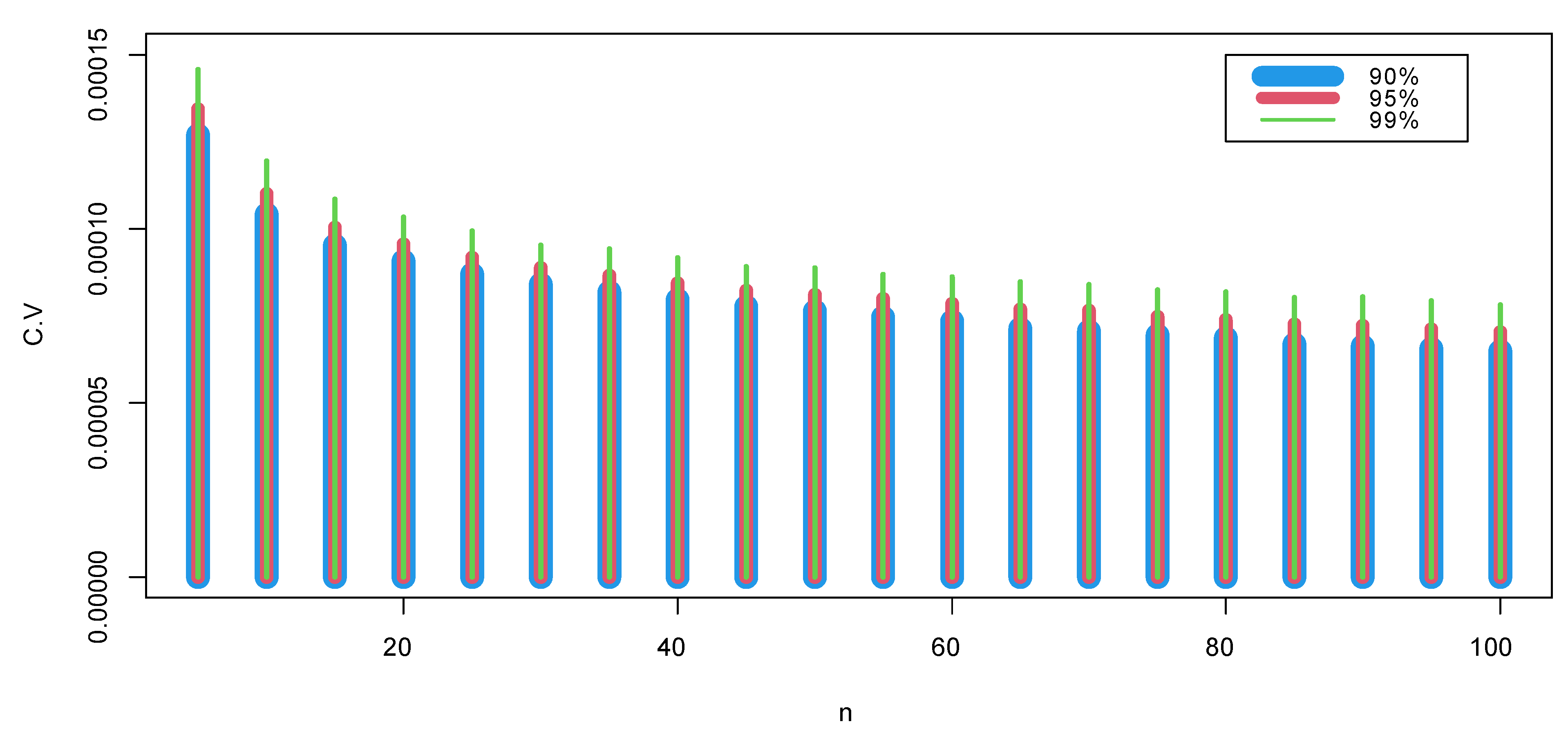
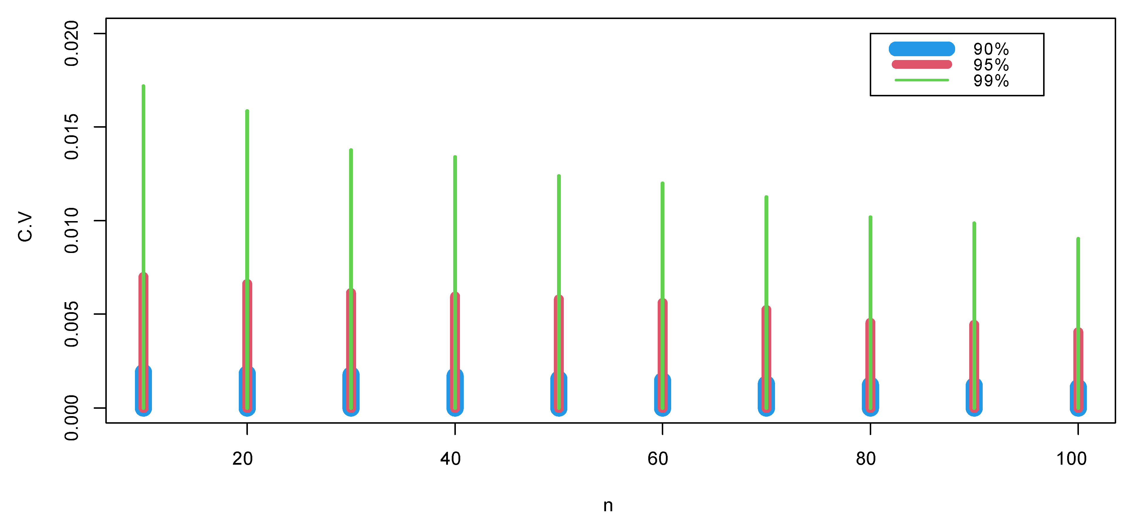
4.1. Critical Points

A critical value (C.V) in statistics refers to a specific point in a distribution of a test statistic; it is conducted to determine whether the null hypothesis may be rejected. This group is referred to as the rejection region or the critical zone. One critical value typically exists for one-sided tests, while two critical values often exist for two-sided tests. The statistical literature does not provide a clear consensus on whether the critical value or probability value method is preferable. Depending on the circumstance and preference, each has benefits and drawbacks. Using 10,000 samples, n = 5(5)100, this part mimics the crucial points of the null Monte Carlo distribution. For 90%, 95%, and 99%, the upper percentile of $\widehat{\Delta }$$\left(0.09\right)$ was identified. As seen in

Table 2. The statistic’s critical values of $\widehat{\Delta }\left(0.09\right)$.

n	$90\%$	$95\%$	$99\%$
5	$0.0001268$	$0.0001343$	$0.0001457$
10	$0.0001041$	$0.0001100$	$0.0001194$
15	$0.0000951$	$0.0001003$	$0.0001085$
20	$0.0000906$	$0.0000955$	$0.0001034$
25	$0.0000868$	$0.0000916$	$0.0000994$
30	$0.0000839$	$0.0000887$	$0.0000952$
35	$0.0000817$	$0.0000865$	$0.0000942$
40	$0.0000795$	$0.0000843$	$0.0000916$
45	$0.0000775$	$0.0000822$	$0.0000890$
50	$0.0000763$	$0.0000810$	$0.0000887$
55	$0.0000745$	$0.0000799$	$0.0000868$
60	$0.0000734$	$0.0000785$	$0.0000861$
65	$0.0000713$	$0.0000769$	$0.0000848$
70	$0.0000706$	$0.0000765$	$0.0000839$
75	$0.0000693$	$0.0000748$	$0.0000824$
80	$0.0000685$	$0.0000738$	$0.0000818$
85	$0.0000667$	$0.0000725$	$0.0000802$
90	$0.0000662$	$0.0000722$	$0.0000805$
95	$0.0000655$	$0.0000711$	$0.0000793$
100	$0.0000647$	$0.0000703$	$0.0000781$

and Figure 1, the critical values rose with higher confidence levels and fell with higher sample sizes.

4.2. The Power Estimates of the Test

The calculations used to establish the minimal sample size for a study are referred to as power estimates in statistics. The probability that the null hypothesis will be correctly rejected, assuming it is true, is known as strength. It is based on four basic factors: power, significance level, sample size, and the number of observations or research participants. The proposed test’s potency was evaluated at the $(1-\alpha )\%$ confidence level, $\alpha =0.05$, using the 10,000 samples provided in

Table 3. Estimates of the power of ${\Delta }_n\left(0.09\right)$.

n	$\mathit{\theta }$	Weibull	Gamma
10	2	$0.9650$	$0.5671$
	3	$0.9997$	$0.8950$
	4	$1.0000$	$0.9568$
20	2	$0.9931$	$0.7116$
	3	$1.0000$	$0.9320$
	4	$1.0000$	$0.9847$
30	2	$0.9994$	$0.7498$
	3	$1.0000$	$0.9560$
	4	$1.0000$	$0.9922$

as a basis. Assume that $\theta$ has proper values for the Weibull distribution (WD), and gamma distribution (GD) at $n=10,20$, and 30, respectively. Table 3 demonstrates that the ${\Delta }_n\left(0.09\right)$ test we employed has adequate power for all other alternatives.

5. Testing for Censored Data

It is recommended to use a test statistic to contrast $H_0$ and $H_1$ with data that have been randomly right-censored. In a life-testing model or a clinical study where patients may be lost (censored) before the completion of a trial, such censored data are frequently the only types of information that are accessible. This hypothetical experiment can be formalized as follows. Assume that n items are checked, with $X_1,X_2,\dots ,X_n$ representing the actual lifespan of each item. We allow $X_1,X_2,\dots ,X_n$ to be independently and identically distributed (i.i.d.) under the assumption of a continuous life distribution, F. Assume that $Y_1,Y_2,\dots ,Y_n$ are (i.i.d.) according to a continuous life distribution, G. Additionally, assume that X and Y are independent variables. The pairs are visible in the randomly right-censored model $(Z_j,{\delta }_j),$ $j=1,\dots ,n,$ where $Z_j=min(X_j,Y_j)$ and

$${\delta }_j=\left\{\begin{array}{ccc}1,\hfill & \mathrm{if}\hfill & Z_j=X_j(\mathrm{j}\text{-}\mathrm{th}\mathrm{observation}\mathrm{is}\mathrm{uncensored})\hfill \\ 0,\hfill & \mathrm{if}\hfill & Z_j=Y_j(\mathrm{j}\text{-}\mathrm{th}\mathrm{observation}\mathrm{is}\mathrm{censored}).\hfill \end{array}\right.$$

(12)

Let $Z_{\left(0\right)}=0<Z_{\left(1\right)}<Z_{\left(2\right)}<\cdots <Z_{\left(n\right)}$ denote the ordered Z and ${\delta }_{\left(j\right)}$ is ${\delta }_j$ corresponding to $Z_{\left(j\right)}.$ The product limit estimator was suggested by Kaplan and Meier [40] using the censored data ($Z_j$, ${\delta }_j$),$j=1,\dots ,n.$

$${\overline{F}}_n\left(X\right)=\prod _{[j:Z(j)\le X]}{\{(n-j)/(n-j+1)\}}^{{\delta }_{\left(j\right)}};X\in [0,Z_{\left(n\right)}].$$

We now propose the following test statistic to compare $H_0:{\widehat{\varphi }}_c=0$ to $H_1:{\widehat{\varphi }}_c>0$, using the randomized right censored data

$$\begin{array}{ccc}\hfill {\widehat{\varphi }}_c& =& [\frac{1}{2}{s}^3-\frac{1}{2}{s}^2]{\mu }_{\left(2\right)}\zeta \left(s\right)+[s^2-s^3]\zeta \left(1\right)\zeta \left(s\right)+[s^2-s^3]\mu \zeta \left(s\right)\hfill \\ & & +[s^3-s^2+1]\zeta \left(s\right)+[s-s^2]\mu -s^2\zeta \left(1\right)+s^2-1,\hfill \end{array}$$

where $\zeta \left(s\right)=\underset{0}{\overset{\infty }{\int }}{e}^{-sx}d{F}_n\left(x\right)$. It is possible to rewrite ${\widehat{\varphi }}_c$ for computational purposes.

$$\begin{array}{ccc}\hfill {\widehat{\varphi }}_c& =& [\frac{1}{2}{s}^3-\frac{1}{2}{s}^2]\mathsf{\Phi }\eta +[s^2-s^3]\mathsf{\tau }\eta +[s^2-s^3]\mathsf{\Omega }\eta \hfill \\ & & +[s^3-s^2+1]\eta +[s-s^2]\mathsf{\Omega }-s^2\tau +s^2-1,\hfill \end{array}$$

where

$$\begin{array}{ccc}\hfill \mathsf{\Omega }& =& \sum _{k=1}^n\left[\prod _{m=1}^{k-1}{C}_m^{\delta \left(m\right)}\left(Z_{\left(k\right)}-Z_{(k-1)}\right)\right],\hfill \\ \hfill \mathsf{\Phi }& =& 2\sum _{i=1}^n\left[\prod _{v=1}^{i-1}{Z}_{\left(i\right)}{C}_v^{\delta \left(v\right)}\left(Z_{\left(i\right)}-Z_{(i-1)}\right)\right],\hfill \\ \hfill \eta & =& \sum _{j=1}^n{e}^{-s{Z}_{\left(j\right)}}[\prod _{p=1}^{j-2}{C}_p^{\delta \left(p\right)}-\prod _{p=1}^{j-1}{C}_p^{\delta \left(p\right)}],\hfill \\ \hfill \tau & =& \sum _{j=1}^n{e}^{-Z_{\left(j\right)}}[\prod _{p=1}^{j-2}{C}_p^{\delta \left(p\right)}-\prod _{p=1}^{j-1}{C}_p^{\delta \left(p\right)}],\hfill \end{array}$$

and

$$d{F}_n\left(Z_j\right)={\overline{F}}_n\left(Z_{j-1}\right)-{\overline{F}}_n\left(Z_j\right),c_k=\left[n-k\right]{\left[n-k+1\right]}^{-1}.$$

The test invariance is achieved by letting

$${\widehat{\Delta }}_c=\frac{{\widehat{\varphi }}_c}{{\overline{Z}}^3},\mathrm{where}\overline{Z}=\sum _{i=1}^n\frac{Z_{\left(i\right)}}{n}.$$

(13)

In

Table 4. The superior percentages of ${\widehat{\Delta }}_c$ with 10,000 replications at $s=0.9$.

n	$90\%$	$95\%$	$99\%$
10	$0.0018839$	$0.0069971$	$0.0171796$
20	$0.0018178$	$0.0066184$	$0.0158503$
30	$0.0017509$	$0.0061387$	$0.0137694$
40	$0.0016926$	$0.0059580$	$0.0133870$
50	$0.0015313$	$0.0057832$	$0.0123716$
60	$0.0014402$	$0.0055886$	$0.0119811$
70	$0.0012656$	$0.0052264$	$0.0112588$
80	$0.0012082$	$0.0045355$	$0.0101906$
90	$0.0011823$	$0.0044339$	$0.0098655$
100	$0.0010760$	$0.0040471$	$0.0090138$

and Figure 2, the crucial percentages of the ${\widehat{\Delta }}_c$ tests for the samples taken $n=10\left(10\right)100$ are displayed. The null Monte Carlo distribution’s crucial values were found using the common exponential distribution, using the Mathematica 12 program at $s=0.9$, and with 10,000 replications. The critical values increased as the confidence level increased and decreased as sample numbers increased, respectively, as shown in Figure 2 and Table 4.

Estimates of the Test Power ${\Delta }_c\left(s\right)$

At a significance level of $\alpha =0.05$, we assessed the test power using the occasion parameter values of $\theta$ based on 10,000 samples, at $n=10,20$ and 30 for the gamma, LFR, and Weibull distributions.

Table 5. Estimates of the power of ${\Delta }_c\left(0.9\right)$.

n	$\mathit{\theta }$	Weibull	LFR	Gamma
10	2	$0.6162$	$0.4496$	$0.3541$
	3	$0.6219$	$0.4843$	$0.3954$
	4	$0.6222$	$0.5035$	$0.4173$
20	2	$0.8289$	$0.6308$	$0.4049$
	3	$0.8328$	$0.6792$	$0.4647$
	4	$0.8351$	$0.7203$	$0.5278$
30	2	$0.9148$	$0.7376$	$0.5497$
	3	$0.9193$	$0.7994$	$0.6949$
	4	$0.9193$	$0.8224$	$0.8167$

exemplifies how the power estimations for this test ${\Delta }_c\left(0.9\right)$ for all other options were suitable.

6. Censored and Uncensored Observations in Applications to Real Data

Data that are controlled (censored) exist, suggesting that some details are omitted or are not comprehensive. Data that have not been filtered are completely known, indicating that they contain all pertinent information. Controlled data can be difficult to analyze statistically since they call for unique approaches and presumptions to deal with missing or insufficient data. Data that are unsupervised (uncensored) do not suffer from these problems, making them easier to analyze. In this Section, the data sets have been discussed and analyzed based on a significance level $\alpha =0.05$.

6.1. Non-Censored Data

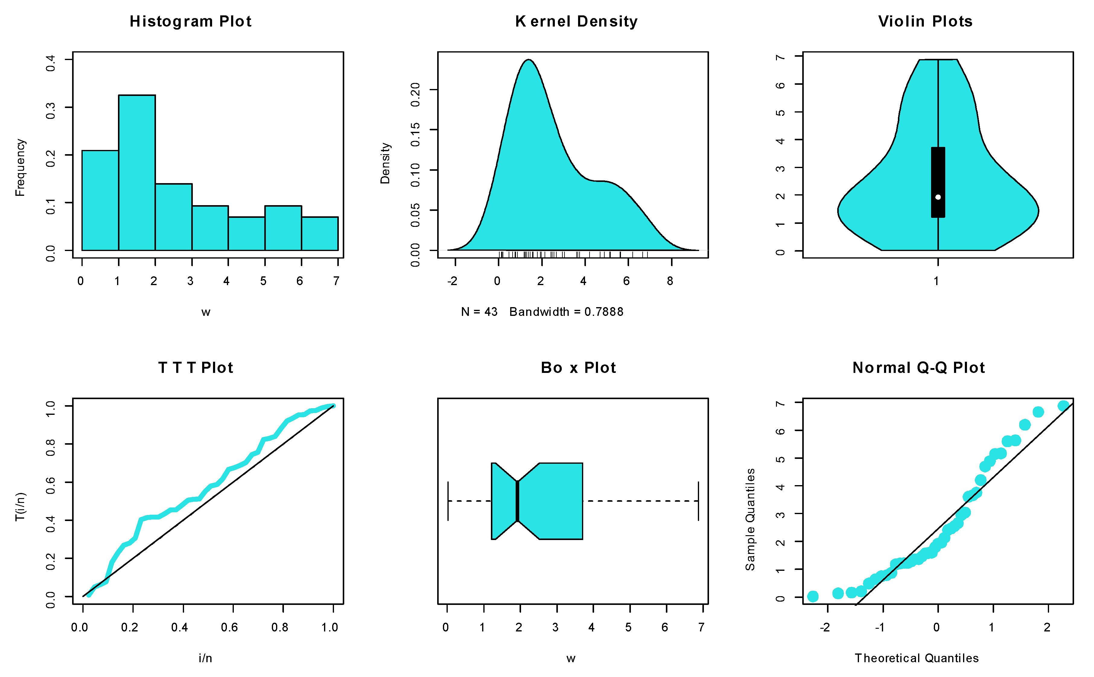
6.1.1. Dataset I: Methylmercury Poisoning

The listed times of death within the week were recorded (using single dosage levels) in a Florida State University experiment to study the effects of methylmercury poisoning on the life spans of fish (see Kochar [41]).

$6.000$	$6.143$	$7.286$	$8.714$	$9.429$
$9.857$	$10.143$	$11.571$	$11.714$	$11.714$

The data representation plots are presented in Figure 3; it was found that there are no extreme observations and the nucleation intensity is asymmetric (left-bimodal-skewed). It was discovered that the critical value, which can be found in Table 2, is exceeded by $\widehat{\Delta }=0.0001122$. We then accept $H_1$, which says that the data collection has $NBRULC$ properties rather than exponential growth.

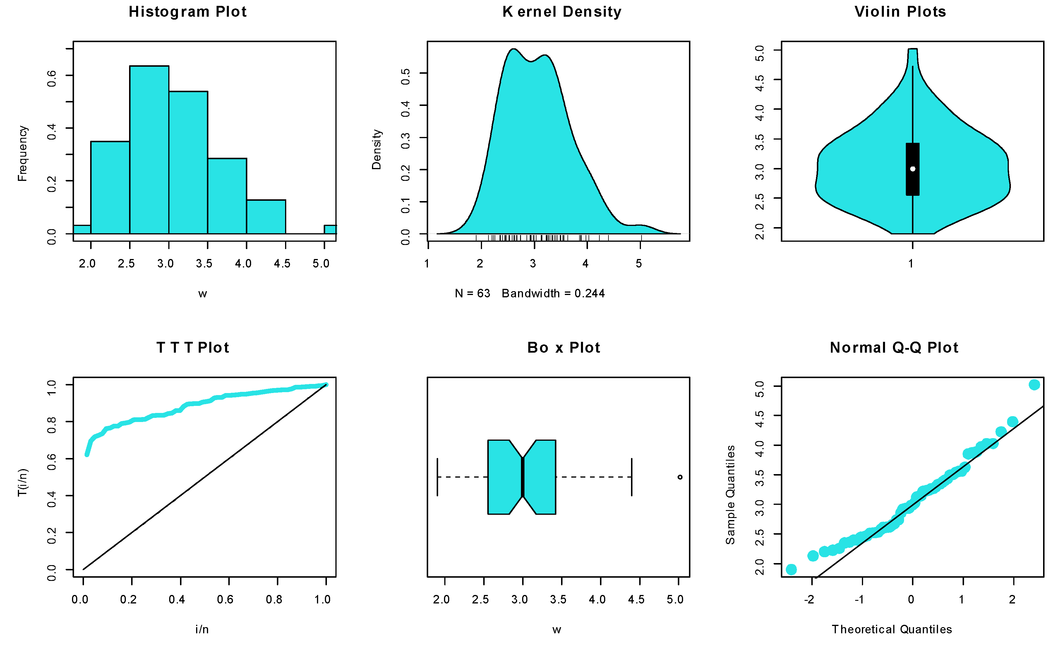
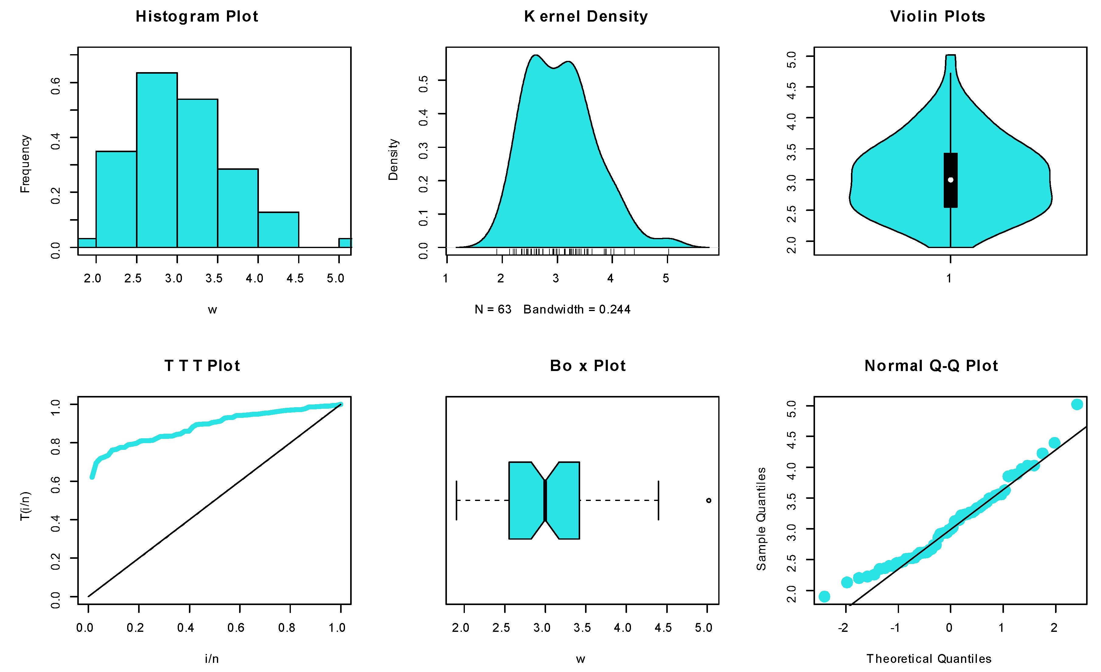
6.1.2. Dataset II: Endurance of Ball Bearings

Pavur et al. [42] took into consideration the information below. The findings of a life test investigation on 23 ball bearings are shown in the following, indicating the number of revolutions (in ten million) until failure.

$1.788$	$2.892$	$3.300$	$4.152$	$4.212$	$4.560$	$4.848$	$5.184$
$5.196$	$5.412$	$5.556$	$6.78$	$6.864$	$6.864$	$6.988$	$8.412$
$9.312$	$9.864$	$10.512$	$10.584$	$12.792$	$12.804$	$17.340$

The data visualization plots are presented in Figure 4. It was reported that there are some extreme observations and the nucleation intensity is asymmetric (bimodal-right-skewed). The dataset’s exponential features are demonstrated by the null hypotheses, which are disproved. When $\widehat{\Delta }=0.0001074$, it is found to exceed the pertinent critical value in Table 2.

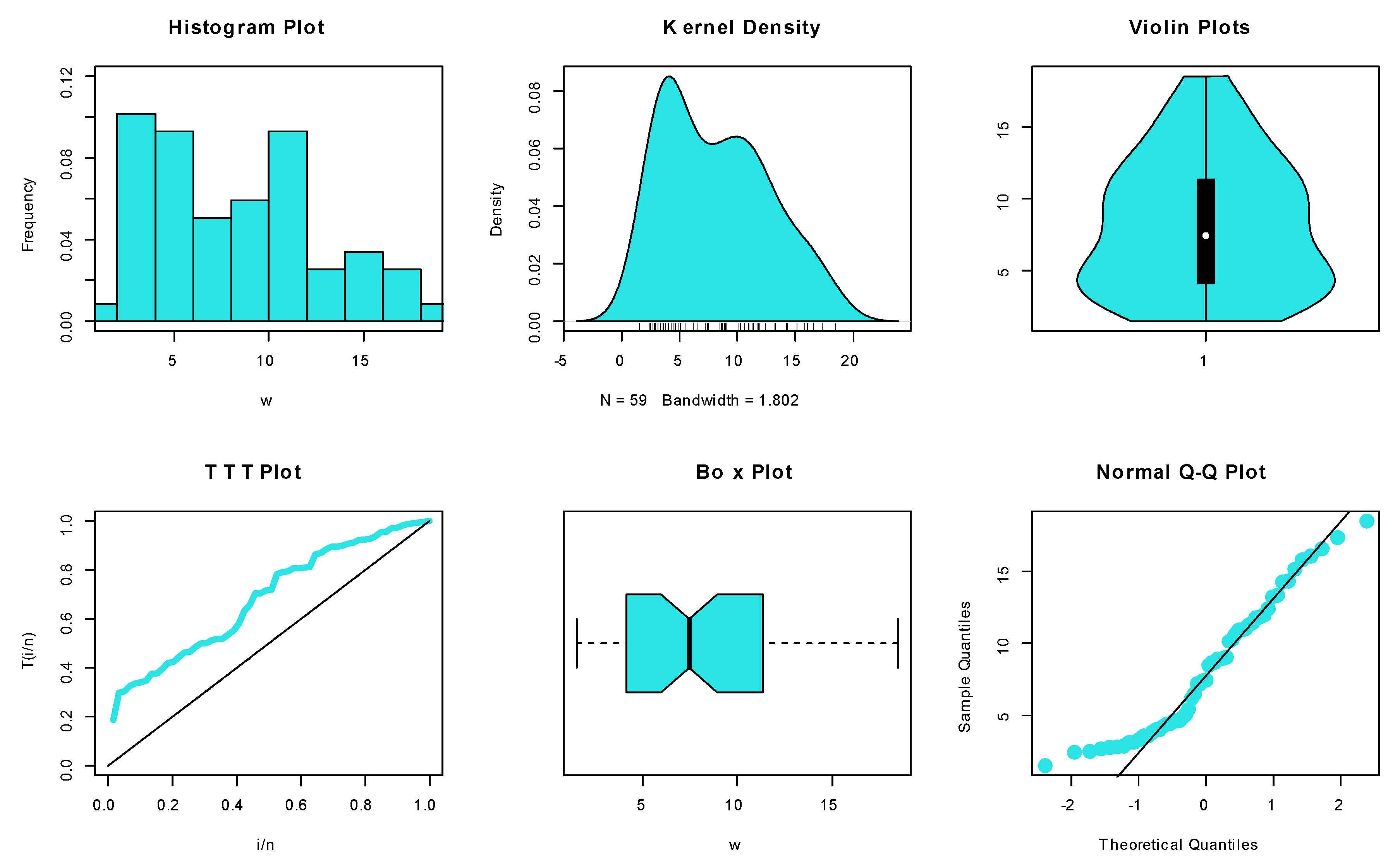
6.1.3. Dataset III: Leukaemia

Check out the information from Abouammoh et al. [43]. These numbers indicate a group of 43 leukemia patients from a Saudi Arabian Ministry of Health hospital, with order values in years, as follows:

$0.315$	$0.496$	$0.699$	$1.145$	$1.208$	$1.263$	$1.414$	$2.025$	$2.036$	$2.162$
$2.211$	$2.370$	$2.532$	$2.693$	$2.805$	$2.910$	$2.912$	$3.192$	$3.263$	$3.348$
$3.348$	$3.427$	$3.499$	$3.534$	$3.718$	$3.751$	$3.858$	$3.986$	$4.049$	$4.244$
$4.323$	$4.323$	$4.381$	$4.392$	$4.397$	$4.647$	$4.753$	$4.929$	$4.973$	$5.074$
$5.203$	$5.274$	$5.384$

The data representation plots are sketched in Figure 5; there are no extreme observations and the nucleation intensity is asymmetric (left-skewed). It was discovered that the critical value, which can be found in Table 2, is exceeded by $\widehat{\Delta }=0.0001222$. We then accept $H_1$, which states that the data collection has $NBRULC$ properties rather than exponential growth.

6.1.4. Dataset IV: Leukaemia

Take a look at the data below, which show the survival periods (in years) following the diagnoses of 43 patients with specific kinds of leukemia (see Kotz and Johnson [44]). The data can be listed as follows:

$0.019$	$0.129$	$0.159$	$0.203$	$0.485$	$0.636$	$0.748$	$0.781$	$0.869$	$1.175$
$1.206$	$1.219$	$1.219$	$1.282$	$1.356$	$1.362$	$1.458$	$1.564$	$1.586$	$1.592$
$1.781$	$1.923$	$1.959$	$2.134$	$2.413$	$2.466$	$2.548$	$2.652$	$2.951$	$3.038$
$3.6$	$3.655$	$3.754$	$4.203$	$4.690$	$4.888$	$5.143$	$5.167$	$5.603$	$5.633$
$6.192$	$6.655$	$6.874$

The data visualization plots are presented in Figure 6; it is clear that there are no extreme observations and the nucleation intensity is asymmetric-bimodal (right-skewed). The dataset’s exponential features are demonstrated by the null hypotheses, which are disproved. When $\widehat{\Delta }=0.0001048$, is found, it exceeds the relevant critical value in Table 2.

6.1.5. Dataset V: Carbon Fibers

Two sets of data that were introduced by Badar and Priest [45] and used by Kundu and Gupta [46] are discussed in this segment. The strength of individual carbon fibers evaluated under tension at gauge lengths of 20 mm is measured in set A using GPA. For set B, individual carbon fibers were tested under stress at gauge lengths of 10 mm; the strength was evaluated in GPA. Size 63 applies to sets A and B. The data visualization plots are listed in Figure 7 and Figure 8.

Dataset A:
$1.312$	$1.314$	$1.479$	$1.552$	$1.700$	$1.803$	$1.861$	$1.865$	$1.944$
$1.958$	$1.966$	$1.997$	$2.006$	$2.021$	$2.027$	$2.055$	$2.063$	$2.098$
$2.140$	$2.179$	$2.224$	$2.240$	$2.253$	$2.270$	$2.272$	$2.274$	$2.301$
$2.301$	$2.359$	$2.382$	$2.382$	$2.426$	$2.434$	$2.435$	$2.478$	$2.490$
$2.511$	$2.514$	$2.535$	$2.554$	$2.566$	$2.570$	$2.586$	$2.629$	$2.633$
$2.642$	$2.648$	$2.684$	$2.697$	$2.726$	$2.770$	$2.773$	$2.800$	$2.809$
$2.818$	$2.821$	$2.848$	$2.880$	$2.954$	$3.012$	$3.067$	$3.084$	$3.090$

In such a case, the estimated value, $\widehat{\Delta }=0.0001036$, exceeds the crucial value shown in Table 2 by a significant amount. Given the $\alpha =0.05$ significant level, it is true because these types of data satisfy the $NBRULC$ characteristic.

Dataset B:
$1.901$	$2.132$	$2.203$	$2.228$	$2.257$	$2.350$	$2.361$	$2.396$	$2.397$
$2.445$	$2.454$	$2.474$	$2.518$	$2.522$	$2.525$	$2.532$	$2.575$	$2.614$
$2.616$	$2.618$	$2.624$	$2.659$	$2.675$	$2.738$	$2.740$	$2.856$	$2.917$
$2.928$	$2.937$	$2.937$	$2.977$	$2.996$	$3.030$	$3.125$	$3.139$	$3.145$
$3.220$	$3.223$	$3.235$	$3.243$	$3.264$	$3.272$	$3.294$	$3.332$	$3.346$
$3.377$	$3.408$	$3.435$	$3.493$	$3.501$	$3.537$	$3.554$	$3.562$	$3.628$
$3.852$	$3.871$	$3.886$	$3.971$	$4.024$	$4.027$	$4.225$	$4.395$	$5.020$

In such a case, the estimated value, $\widehat{\Delta }=0.0001131$, exceeds the crucial value shown in Table 2 by a significant amount. Given the $\alpha =0.05$ significant level, it is true because these types of data satisfy the $NBRULC$ characteristic.

6.1.6. Dataset VI: COVID-19

According to EL-Sagheer et al. [47], this information indicates the fatality rate for COVID-19 in the Netherlands from 31 March to 30 April 2020. The information is as follows:

$14.918$	$10.656$	$12.274$	$10.289$	$10.832$	$7.099$	$5.928$	$13.211$
$7.968$	$7.584$	$5.555$	$6.027$	$4.097$	$3.611$	$4.960$	$7.498$
$6.940$	$5.307$	$5.048$	$2.857$	$2.254$	$5.431$	$4.462$	$3.883$
$3.461$	$3.647$	$1.974$	$1.273$	$1.416$	$4.235$

The data visualization plots are presented in Figure 9. It was discovered that the critical value, which can be found in Table 2, is exceeded by $\widehat{\Delta }=0.0001081$. We then accept $H_1$, which states that the data collection has $NBRULC$ properties rather than exponential growth.

6.1.7. Dataset VII: COVID-19

According to Almongy et al. [48], this information indicates the fatality rate for COVID-19 in Italy from 27 February to 27 April 2020. The information is as follows:

$4.571$	$7.201$	$3.606$	$8.479$	$11.410$	$8.961$	$10.919$	$10.908$	$6.503$
$18.474$	$11.010$	$17.337$	$16.561$	$13.226$	$15.137$	$8.697$	$15.787$	$13.333$
$11.822$	$14.242$	$11.273$	$14.330$	$16.046$	$11.950$	$10.282$	$11.775$	$10.138$
$9.037$	$12.396$	$10.644$	$8.646$	$8.905$	$8.906$	$7.407$	$7.445$	$7.214$
$6.194$	$4.640$	$5.452$	$5.073$	$4.416$	$4.859$	$4.408$	$4.639$	$3.148$
$4.040$	$4.253$	$4.011$	$3.564$	$3.827$	$3.134$	$2.780$	$2.881$	$3.341$
$2.686$	$2.814$	$2.508$	$2.450$	$1.518$

The data representation plots are listed in Figure 10. The dataset’s exponential features are demonstrated by the null hypotheses, which are disproved. When $\widehat{\Delta }=0.0001027$, it is determined to exceed the critical value specified in Table 2.

6.1.8. Dataset VIII: Wind Speed

We used the following dataset, which was originally obtained from NCDC. These data represent the wind speed measured in knots for the first sample (set A) for 23 days and the second sample for 25 days (see, Ghazal et al. [49]).

Dataset A:
$8.6$	$3.8$	$5.4$	$4.4$	$2.2$	$3.8$	$4.5$	$6.3$
$3.4$	$4.1$	$3.8$	$8.6$	$13.0$	$11.3$	$12.4$	$12.4$
$5.0$	$3.4$	$3.8$	$5.3$	$3.6$	$5.8$	$4.2$

The data visualization plots are presented in Figure 11 (set A); there are no extreme observations and the nucleation intensity is asymmetric-bimodal (right-skewed).

In such a case, the estimated value, $\widehat{\Delta }=0.0001084$, exceeds the crucial value shown in Table 2 by a significant amount. Given the $\alpha =0.05$ significant level, it is true because these types of data satisfy the $NBRULC$ characteristic.

Dataset B:
$2.4$	$2.9$	$3.3$	$3.4$	$3.5$	$3.7$	$3.8$	$3.9$	$4.0$
$4.1$	$4.2$	$4.5$	$4.6$	$4.8$	$5.1$	$5.3$	$5.5$	$6.0$
$6.2$	$6.5$	$7.8$	$8.2$	$8.4$	$9.4$	$10.9$

The data visualization plots are presented in Figure 12 (set B); there are some extreme observations and the nucleation intensity is asymmetric-multimodal (right-skewed). In such a case, the estimated value, $\widehat{\Delta }=0.0001183$, exceeds the crucial value shown in Table 2 by a significant amount. Considering the significance level of $\alpha =0.05$, it can be concluded that these types of data satisfy the $NBRULC$ characteristic.

6.2. Censored Data

6.2.1. Dataset IX: Lung Cancer

The following data represent the number of weeks that 61 individuals, who received cyclophosphamide for incurable lung cancer, survived and were considered in the studies by Lagakos and Williams [50] and Lee and Wolfe [51]. For the patients whose treatments were stopped due to a deteriorating condition, there are 28 censored observations and 33 uncensored observations.

• Censored observations:

0.14	0.14	0.29	0.43	0.57	0.57	1.86	3.00	3.00	3.29
3.29	6.00	6.00	6.14	8.71	10.57	11.86	15.57	16.57	17.29
18.71	21.29	23.86	26.00	27.57	32.14	33.14	47.29

• Uncensored observations:

0.43	2.86	3.14	3.14	3.43	3.43	3.71	3.86	6.14	6.86	9.00
9.43	10.71	10.86	11.14	13.00	14.43	15.71	18.43	18.57	20.71	29.14
29.71	40.57	48.57	49.43	53.86	61.86	66.57	68.71	68.96	72.86	72.86

When considering all available survival statistics, both censored and uncensored, we discover that Table 4’s essential value exceeds our conclusion, which is ${\Delta }_c\left(0.9\right)=-0.00099279$. We can, therefore, clearly see the exponential nature of the data.

6.2.2. Dataset XI: Melanoma

Consider the information from Susarla and Van Ryzin [52]. These numbers represent the survival rates of 46 melanoma patients. Among them, 35 (non-censored material) have complete lifetime information. The following observations have been redacted, in order, as follows:

13	14	19	19	20	21	23	23	25	26
26	27	27	31	32	34	34	37	38	38
40	46	50	53	54	57	58	59	60	65
65	66	70	85	90	98	102	103	110	118
124	130	136	138	141	234

The following is the hierarchy of the censored observations:

16	21	44	50	55	67	73	76	80	81
86	93	100	108	114	120	124	125	129	130
132	134	140	147	148	151	152	152	158	181
190	193	194	213	215

If we take into account both censored and uncensored survival statistics, the essential value in Table 4 exceeds our outcome, which is ${\Delta }_c\left(0.9\right)=-2.65634\times {10}^{-23}$. The exponential properties of the data are, therefore, evident to us.

7. Conclusions

An exponential comparison of different life distributions has garnered much attention. Based on the goodness-of-fit technique, we introduced a new test statistic in this study to evaluate the exponential versus non-exponential NBRULC class of life distributions. For the uncensored and censored data, Table 1 and Table 3 calculated and tabulated the critical values for this test. The efficiency of the Pitman asymptotic efficiency was discussed, and power estimates were simulated for families of the most common age distribution in reliability. The Monte Carlo critical points for the null distribution were simulated. Moreover, the power estimations of this test were computed for a few typical alternative distributions. Several key values were listed along with the power estimates for the censored and uncensored data for this test; moreover, the issue of properly suppressed data was also discussed. To illustrate the usefulness of the recommended test in the reliability analyses of censored and uncensored data, this paper covered several applications.

References

1. Bryson, M.C.; Siddiqui, M.M. Some criteria for aging. J. Am. Stat. Assoc. 1969, 64, 1472–1483. [Google Scholar] [CrossRef]
2. Bhattacharyya, D.; Khan, R.A.; Mitra, M. A test of exponentiality against DMTTF alternatives via L-statistics. Stat. Probab. Lett. 2020, 165, 108853. [Google Scholar] [CrossRef]
3. Barlow, R.E.; Proschan, F. Statistical Theory of Reliability and Life Testing; To Begin With: Silver Spring, MD, USA, 1981. [Google Scholar]
4. Klefsjo, B. The HNBUE and HNWUE classes of life distributions. Nav. Res. Logist. 1982, 29, 331–344. [Google Scholar] [CrossRef]
5. Khan, R.A.; Bhattacharyya, D.; Mitra, M. Exact and asymptotic tests of exponentiality against nonmonotonic mean time to failure type alternatives. Stat. Pap. 2021, 62, 3015–3045. [Google Scholar] [CrossRef]
6. Kumazawa, Y. A class of tests statistics for testing whether new is better than used. Commun. Stat. Theory Methods 1983, 12, 311–321. [Google Scholar] [CrossRef]
7. Mahmoud, M.A.W.; EL-Sagheer, R.M.; Etman, W.B.H. Testing exponentiality against new better than renewal used in Laplace transform order. J. Stat. Appl. Probab. 2016, 5, 279–285. [Google Scholar] [CrossRef]
8. Mahmoud, M.A.W.; EL-Sagheer, R.M.; Etman, W. B H. Moments inequalities for NBRUL distributions with hypotheses testing applications. Austrian J. Stat. 2018, 47, 95–104. [Google Scholar]
9. Majumder, P.; Mitra, M. A test for detecting Laplace order dominance and related Bahadur efficiency issues. Stat. Pap. 2019, 60, 1921–1937. [Google Scholar] [CrossRef]
10. Bhattacharyya, D.; Khan, R.A.; Mitra, M. Tests for Laplace order dominance with applications to insurance data. Insur. Math. Econ. 2021, 99, 163–173. [Google Scholar] [CrossRef]
11. Navarro, J. Preservation of DMRL and IMRL aging classes under the formation of order statistics and coherent systems. Stat. Probab. Lett. 2018, 137, 264–268. [Google Scholar] [CrossRef]
12. Abu-Youssef, S.E.; Hassan, E.M.A.; Gerges, S.T. A new nonparametric class of life distributions based on ordering moment generating approach. J. Stat. Appl. Probab. Lett. 2020, 7, 151–162. [Google Scholar]
13. Ghosh, S.; Mitra, M. A new test for exponentiality against HNBUE alternatives. Commun. Stat. Theory Methods 2020, 49, 27–43. [Google Scholar] [CrossRef]
14. Navarro, J.; Pellerey, F. Preservation of ILR and IFR aging classes in sums of dependent random variables. Appl. Stoch. Model. Bus. Ind. 2022, 38, 240–261. [Google Scholar] [CrossRef]
15. El-Morshedy, M.; Al-Bossly, A.; EL-Sagheer, R.M.; Almohaimeed, B.; Etman, W.B.H.; Eliwa, M.S. A moment inequality for the NBRULC class: Statistical properties with applications to model asymmetric data. Symmetry 2022, 14, 2353. [Google Scholar] [CrossRef]
16. EL-Sagheer, R.M.; Abu-Youssef, S.E.; Sadek, A.; Omar, K.M.; Etman, W.B.H. Characterrization and testing NBRUL class of life distributions based on Laplace transform technique. J. Stat. Appl. Probab. 2022, 11, 1–14. [Google Scholar]
17. Gadallah, A.M.; Mohammed, B.I.; Al-Babtain, A.A.; Khosa, S.K.; Kilai, M.; Yusuf, M.; Bakr, M.E. Modeling various survival distributions using a nonparametric hypothesis testing based on Laplace transform approach with some real applications. Comput. Math. Methods Med. 2022, 2022, 5075716. [Google Scholar] [CrossRef]
18. Mansour, M.M.M. Assessing treatment methods via testing exponential property for clinical data. J. Stat. Appl. Probab. 2022, 11, 109–113. [Google Scholar]
19. Ghosh, S.; Mitra, M. A weighted integral approach to testing against HNBUE alternatives. Stat. Probab. Lett. 2017, 129, 58–64. [Google Scholar] [CrossRef]
20. Majumder, P.; Mitra, M. A test of exponentiality against alternatives. J. Nonparametr. Stat. 2019, 31, 794–812. [Google Scholar] [CrossRef]
21. Lai, C.D.; Xie, M. Stochastic Ageing and Dependence for Reliability; Springer: New York, NY, USA, 2006. [Google Scholar]
22. Etman, W.B.H.; EL-Sagheer, R.M.; Abu-Youssef, S.E.; Sadek, A. On some characterizations to NBRULC class with hypotheses testing application. Appl. Math. Inf. Sci. 2022, 16, 139–148. [Google Scholar]
23. Ghosh, S.; Majumder, P. A moment inequality for decreasing mean time to failure distributions with hypothesis testing application. J. Stat. Comput. Simul. 2022, 92, 2875–2890. [Google Scholar] [CrossRef]
24. Bakr, M.E.; Al-Babtain, A.A. Non-parametric hypothesis testing for unknown aged class of life distribution using real medical data. Axioms 2023, 12, 369. [Google Scholar] [CrossRef]
25. Ghosh, S.; Mitra, M. On the exact distribution of generalized Hollander-Proschan type statistics. Commun. Stat. Simul. Comput. 2022, 51, 5051–5067. [Google Scholar] [CrossRef]
26. Alqifar, H.; Eliwa, M.S.; Etman, W.B.H.; El-Morshedy, M.; Al-Essa, L.A.; EL-Sagheer, R.M. Reliability class testing and hypothesis specification: NBRULC-t characterizations with applications for medical and engineering data modeling. Axioms 2023, 12, 414. [Google Scholar] [CrossRef]
27. Mahmoud, M.A.W.; Abdul Alim, N.A. A goodness of fit approach to NBURFR and NBARFR classes. Econ. Qual. Control 2006, 21, 59–75. [Google Scholar] [CrossRef]
28. Kayid, M.; Diab, L.S.; Alzughaibi, A. Testing NBU (2) class of life distribution based on goodness of fit approach. J. King Saud-Univ.-Sci. 2010, 22, 241–245. [Google Scholar] [CrossRef] [Green Version]
29. Bera, S.; Bhattacharyya, D.; Khan, R.A.; Mitra, M. Test for harmonic mean residual life function: A goodness of fit approach. Math. Comput. Simul. 2023, 203, 58–70. [Google Scholar] [CrossRef]
30. Mahmoud, M.A.W.; Diab, L.S.; Radi, D.M. Testing exponentiality against RNBUL class of life distribution based on goodness of fit. J. Stat. Appl. Probab. 2019, 8, 57–66. [Google Scholar] [CrossRef]
31. Abu-Youssef, S.E.; Ali, N.S.A.; Bakr, M.E. Used better than aged in mgf ordering class of life distribution with application of hypothesis testing. J. Stat. Appl. Probab. Lett. 2020, 7, 23–32. [Google Scholar]
32. Bakr, M.E.; Nagy, M.; Al-Babtain, A.A. Non-parametric hypothesis testing to model some cancers based on goodness of fit. AIMS Math. 2022, 7, 13733–13745. [Google Scholar] [CrossRef]
33. Abu-Youssef, S.E.; El-Toony, A.A. A new class of life distribution based on Laplace transform and It’s applications. Inf. Sci. Lett. 2022, 11, 355–362. [Google Scholar]
34. Abu-Youssef, S.E.; Gerges, S.T. Based on the goodness of fit approach, a new test statistics for testing NBUCmgf class of life distributions. Pak. J. Stat. 2022, 38, 129–144. [Google Scholar]
35. Etman, W.B.H.; El-Morshedy, M.; Eliwa, M.S.; Almohaimeed, A.; EL-Sagheer, R.M. A new reliability class-test statistic for life distributions under convolution, mixture and homogeneous shock model: Characterizations and applications in engineering and medical fields. Axioms 2023, 12, 331. [Google Scholar] [CrossRef]
36. Lee, A.J. U-Statistics-Theorem and Practice. In Statistics Textbooks Monographs; Marcel Dekker: New York, NY, USA, 1990; p. 110. [Google Scholar]
37. Mugdadi, A.R.; Ahmad, I.A. Moment inequalities derived from comparing life with its equilibrium form. J. Stat. Plan. Inference 2005, 134, 303–317. [Google Scholar] [CrossRef]
38. Kango, A.I. Testing for new is better than used. Commun. Stat. Theory Methods 1993, 12, 311–321. [Google Scholar]
39. Abdel Aziz, A.A. On testing exponentiality against RNBRUE alternatives. Appl. Math. Sci. 2007, 35, 1725–1736. [Google Scholar]
40. Kaplan, E.L.; Meier, P. Nonparametric estimation from incomplete observation. J. Am. Stat. Assoc. 1958, 53, 457–481. [Google Scholar] [CrossRef]
41. Kocha, S.C. Testing exponenttality against monotone failure rate average. Commun. Stat. Theory Methods 1985, 14, 381–392. [Google Scholar] [CrossRef]
42. Pavur, R.J.; Edgeman, R.L.; Scott, R.C. Quadratic statistics for the goodness-of-fit test of the inverse Gaussian distribution. IEEE Trans. Reliab. 1992, 41, 118–123. [Google Scholar] [CrossRef]
43. Abouammoh, A.M.; Abdulghani, S.A.; Qamber, I.S. On partial orderings and testing of new better than renewal used classes. Reliab. Eng. Syst. Saf. 1994, 43, 37–41. [Google Scholar] [CrossRef]
44. Kotz, S.; Johnson, N.L. Encyclopedia of Statistical Sciences; Wiley: New York, NY, USA, 1983. [Google Scholar]
45. Bader, M.G.; Priest, A.M. Statistical aspects of fibre and bundle strength in hybrid composites. In Progress in Science and Engineering of Composites; Hayashi, T., Kawata, K., Umekawa, S., Eds.; ICCM-IV: Tokyo, Japan, 1982; pp. 1129–1136. [Google Scholar]
46. Kundu, D.; Gupta, R.D. Estimation of P[Y<X] for Weibull Distributions. IEEE Trans. Reliab. 2006, 55, 270–280. [Google Scholar]
47. EL-Sagheer, R.M.; Eliwa, M.S.; Alqahtani, K.M.; EL-Morshedy, M. Asymmetric randomly censored mortality distribution: Bayesian framework and parametric bootstrap with application to COVID-19 data. J. Math. 2022, 2022, 8300753. [Google Scholar] [CrossRef]
48. Almongy, H.M.; Almetwally, E.M.; Aljohani, H.M.; Alghamdi, A.S.; Hafez, E.H. A new extended rayleigh distribution with applications of COVID-19 data. Results Phys. 2021, 23, 104012. [Google Scholar] [CrossRef] [PubMed]
49. Ghazal, M.G.M.; EL-Sagheer, R.M.; Mahmoud, M.A.W.; Al-Babtain, A.A.; Bakr, M.E.; Hasaballah, M.M. Inference for two populations 3-Burr-XII in presence of joint progressive censoring. Hindawi Complex. 2022, 2022, 6171714. [Google Scholar]
50. Lagakos, S.W.; Williams, J.S. Models for censored survival analysis: A cone class of variable-sum models. Biometrika 1978, 65, 181–189. [Google Scholar] [CrossRef]
51. Lee, S.Y.; Wolfe, R.A. A simple test for independent censoring under the proportional hazards model. Biometrics 1998, 54, 1176–1182. [Google Scholar] [CrossRef]
52. Susarla, V.; Vanryzin, J. Empirical Bayes estimations of a survival function right censored observation. Ann. Stat. 1978, 6, 710–755. [Google Scholar] [CrossRef]
Figure 1. Relationship between the sample size, the level of confidence, and the critical values.
Mathematics 11 02805 g001
Figure 2. Relationship between the sample size, the level of confidence, and the critical values.
Mathematics 11 02805 g002
Figure 3. Non-parametric plots for dataset I.
Mathematics 11 02805 g003
Figure 4. Non-parametric plots for dataset II.
Mathematics 11 02805 g004
Figure 5. Non-parametric plots for dataset III.
Mathematics 11 02805 g005
Figure 6. Non-parametric plots for dataset IV.
Mathematics 11 02805 g006
Figure 7. Non-parametric plots for set A of dataset V.
Mathematics 11 02805 g007
Figure 8. Non-parametric plots for set B of dataset V.
Mathematics 11 02805 g008
Figure 9. Non-parametric plots for dataset VI.
Mathematics 11 02805 g009
Figure 10. Non-parametric plots for dataset VII.
Mathematics 11 02805 g010
Figure 11. Non-parametric plots for set A of dataset VIII.
Mathematics 11 02805 g011
Figure 12. Non-parametric plots for set B of dataset VIII.
Mathematics 11 02805 g012