Mixture Basis Function Approximation and Neural Network Embedding Control for Nonlinear Uncertain Systems with Disturbances

Abstract

A neural network embedding learning control scheme is proposed in this paper, which addresses the performance optimization problem of a class of nonlinear system with unknown dynamics and disturbance by combining with a novel nonlinear function approximator and an improved disturbance observer (DOB). We investigated a mixture basic function (MBF) to approximate the unknown nonlinear dynamics of the system, which allows an approximation in a global scope, replacing the traditional radial basis function (RBF) neural networks technique that only works locally and could be invalid beyond some scope. The classical disturbance observer is improved, and some constraint conditions thus are no longer needed. A neural network embedding learning control scheme is exploited. An arbitrary type of neural network can be embedded into a base controller, and the new controller is capable of optimizing the control performance by tuning the parameters of neural network and satisfying the Lyapunov stability simultaneously. Simulation results verify the effectiveness and advantage of our proposed methods.

1. Introduction

With the need of a practical control system in social production and the development of control theory, the high performance control of nonlinear systems, such as motor torque control [1], UAV control [2], and robot control [3] has become an important research problem in control science and applications [4]. How to compensate for the uncertainties and disturbances in the model is the focus of this research in nonlinear systems. Therefore, the research on uncertainty compensation, disturbance suppression and performance optimization is of great significance [5].

For the unknown nonlinear function in the model, the widely adopted method is the function approximator, which is used to estimate and compensate for the unknown nonlinear function. The radial basis function (RBF) is often used as a function approximator to model unknown nonlinear functions. For example, a fast algorithm for characteristics of contactors based on the RBF neural network approximate model is proposed in [6]. In [7], the nonlinear system of industrial process is modeled by using the approximation ability of RBF. In [8], RBF is used to approximate and compensate for the nonlinearity and uncertainty in the robot model. In [9], the model uncertainties of a combine harvester, including unknown vehicle parameters, variable trailer mass and external disturbances, are compensated by an effective combination of a RBF neural network and an adaptive robust control law. In addition, other approximation methods, such as fuzzy system, are also widely proposed. For example, a fuzzy logic system is used to approximate the unknown nonlinear function and the unknown control gain function of the model in [10]. A fuzzy adaptive method is proposed in [11] to compensate unknown nonlinear functions in nonlinear systems with nonstrict feedback, and it is assumed that unknown functions must meet the monotonically increasing nature, which limits the applicability of the control method in practical engineering. The above methods are based on the Gaussian function as the basis function to approximate and compensate for the unknown nonlinear function. Taking the RBF neural network method as an example, RBF approximates unknown nonlinear functions in a local range, called local approximation, which means that the farther the neuron’s input is from the center of the RBF, the lower the activation of the neuron. As a result, the approximation of the unknown nonlinear function is realized only by the scope around the function central point of radial functions, while the distant radial functions do not work, resulting in a large tracking error. Furthermore, the multi-dimensional Taylor network is used for the problem of approximation as the approximation of nonlinear terms and disturbances in the system model to compensate for lumped non-linearities in [12], and it only is taken into account to lessen the computational complexity and improve the real-time performance for quadrotor control, not the global approximation for an unknown nonlinear function.

It is generally known that practical systems are often subject to external disturbances, which can cause the performance degradation and instability of systems. Thus, for the disturbance problem in the system model, active disturbance rejection control (ADRC) technology and various disturbance observers are widely adopted to solve the disturbance problems in the system model. For example, In [13,14], ADRC is used to estimate and compensate for the lumped disturbance in the system. In [15], an iterative learning disturbance observer is designed to solve the complex disturbance problems in spacecraft. In [16], a sliding mode disturbance observer is designed to deal with disturbances in nonlinear systems. In [17,18], the disturbance observer is used to deal with the problem of multiple disturbances in servo systems. The above research has made some achievements in the compensation of the disturbance problem, and the dynamic performance of the system is improved to some extent. However, for the above disturbance observers, it is necessary to assume that the disturbance in the control model is constant or slowly changes, which means the disturbance derivative is zero or approximately zero. When the disturbance changes rapidly, the disturbance observer is difficult to track the disturbance, so it is impossible to compensate for the disturbance.

In recent years, deep learning techniques [19,20] have been developed significantly, and neural networks have become an important tool for nonlinear system control due to their approximation, learning, and adaptive capabilities [21,22,23]. Aiming at system performance optimization issues, in [24], Chebyshev neural networks are employed to approximate the unknown nonlinear functions in the system, combined with sliding mode control to achieve adaptive optimal control. In [25], a neural network as a discriminator to obtain the dynamics of the system and a nonlinear network control system based on neural dynamic programming are designed to achieve stochastic optimal control in a finite time frame; however, due to the existence of certain errors in the discriminative process, it will have an impact on the system stability. In order to solve the problem, some scholars construct the objective function with tracking error to optimize the controlling performance by the neural network. For example, in [26], neural networks and reinforcement learning are adopted to optimize the tracking control of a nonlinear dynamic system by constructing a desired tracking trajectory error term. In [27], the neural network observer is used to estimate the unknown back-electromotive force in the permanent magnet synchronous motors and is combined with the augmented feedforward controller to achieve optimal control of the nonlinear system by adjusting the neural network weights. However, the observer has some observation error, which affects the trajectory tracking accuracy. In [28], a self-organized recursive RBF neural network can achieve predictive control of the nonlinear model, based on which the optimal controller is found by the gradient method and the learning capability of the neural network. In the above methods, the neural network is used as an approximator or discriminator of the unknown dynamics to indirectly reduce the tracking error and thus achieve performance optimization. Although the above methods play a certain role in optimizing the control performance of the system, the learning ability of neural network is not fully excavated, the approximation error of neural network is not considered in most of the optimization process, and its stability analysis is more complex.

In summary, the problems of controlling performance optimization for the nonlinear uncertain system with disturbance have been solved to a certain extent but still need to be improved. Based on the above problems, a neural network embedding control method based on the mixture basis function (MBF) and an improved disturbance observer is proposed for uncertain dynamic systems. The main contribution of this paper is as follows:

(1)

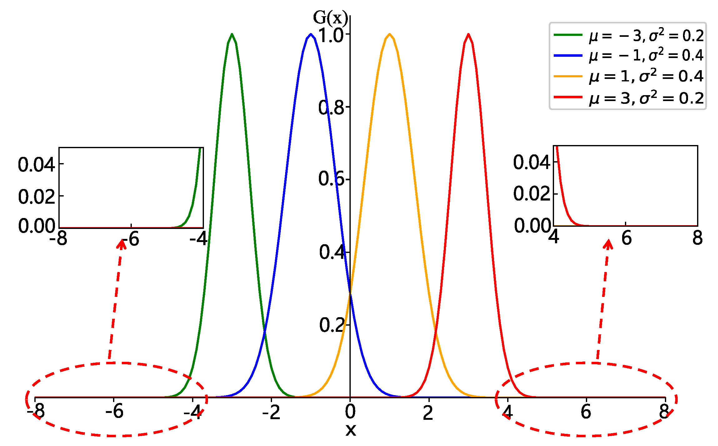
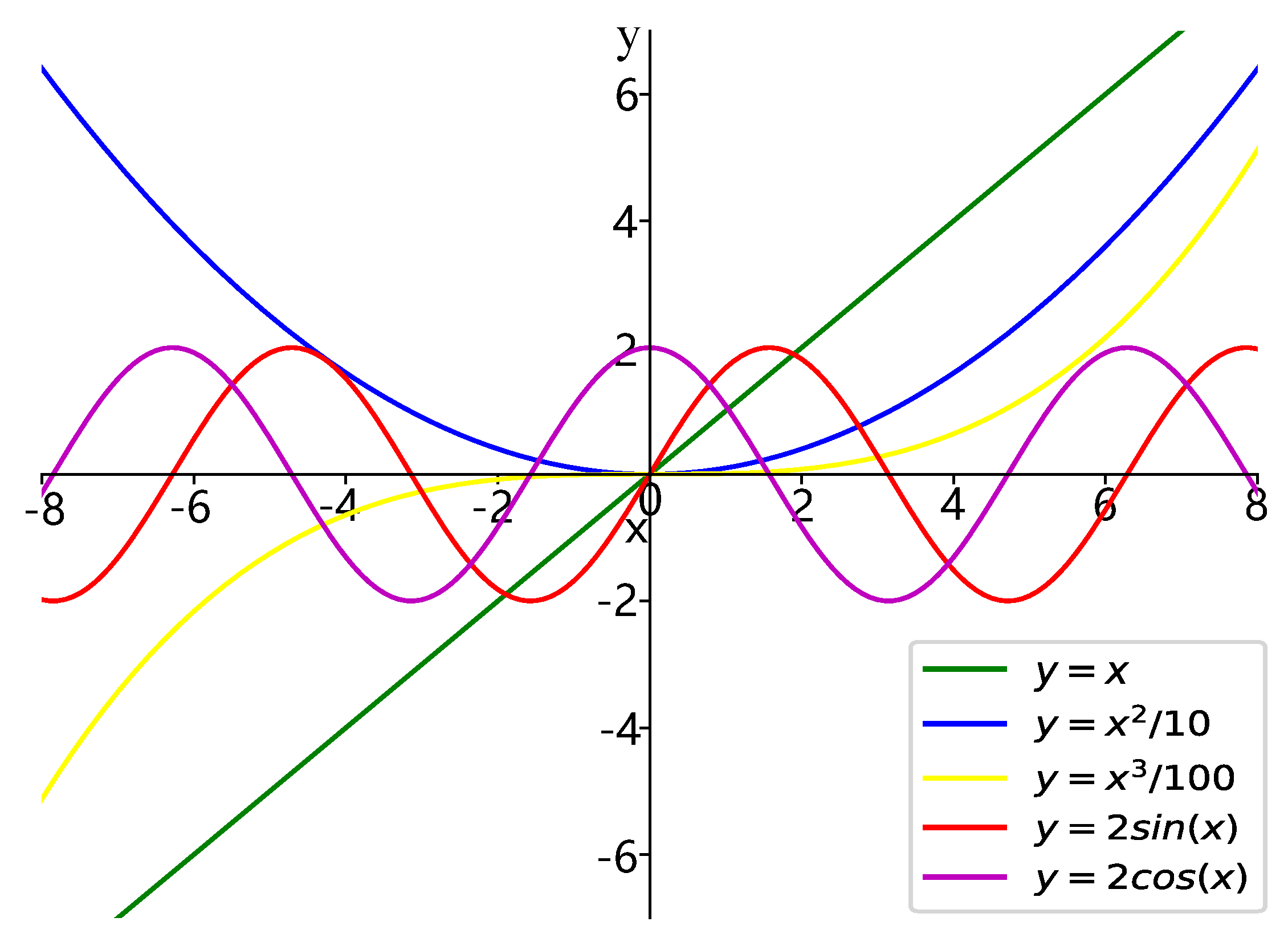
A novel approximation method is proposed that allows an approximate nonlinear function of the system globally rather than existing methods that are only local. Hence, in the practical application, when some state oversteps the limited range, the RBF will fail to approximate, whereas MBF will have not have this problem.

(2)

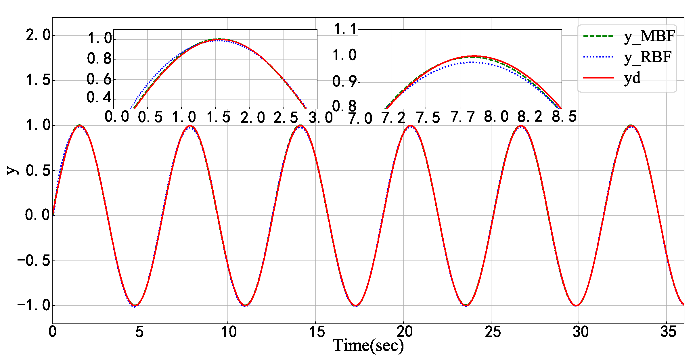
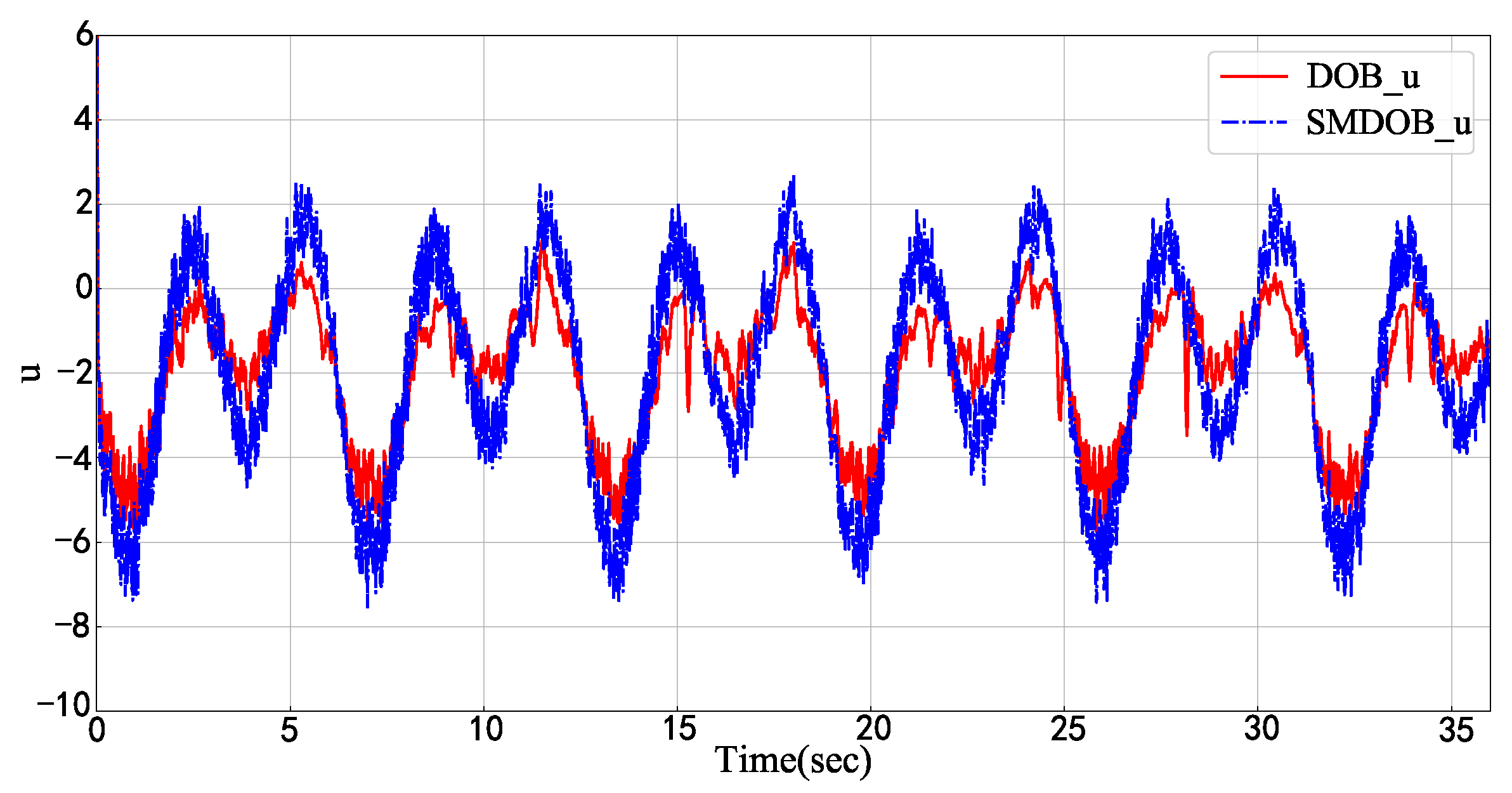
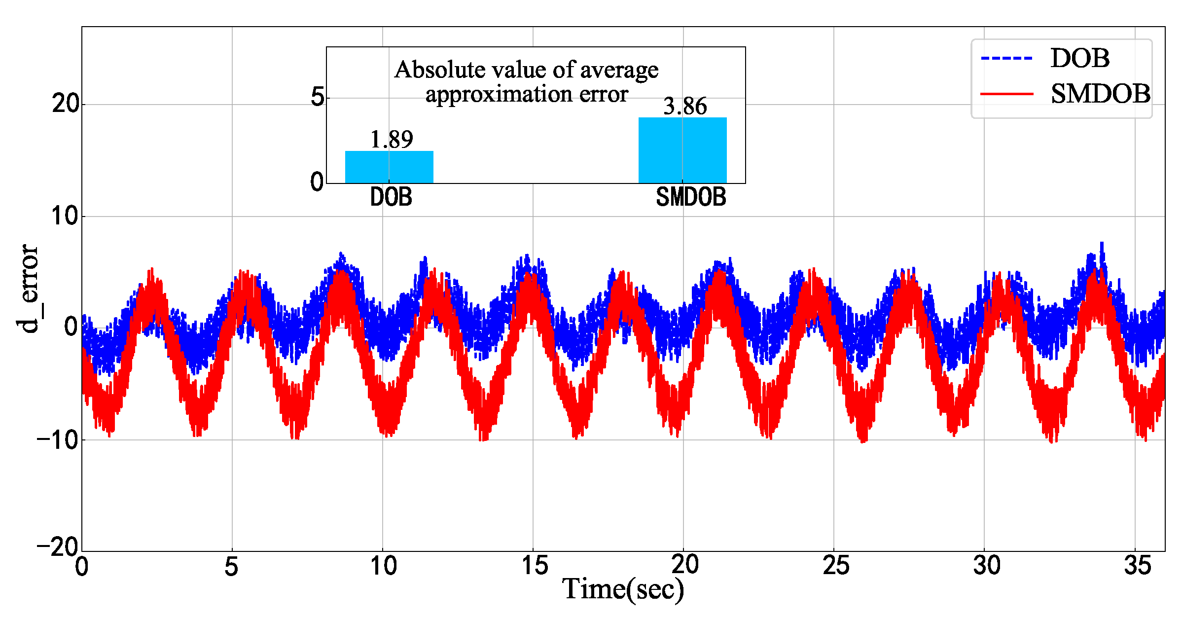
An improved disturbance observer is designed for the disturbance estimation problem that relaxes the restriction condition about the rate of disturbance changing and thus expands the practical application range of the disturbance observer. Meanwhile, the simulation results show that our method has superior estimation performance.

(3)

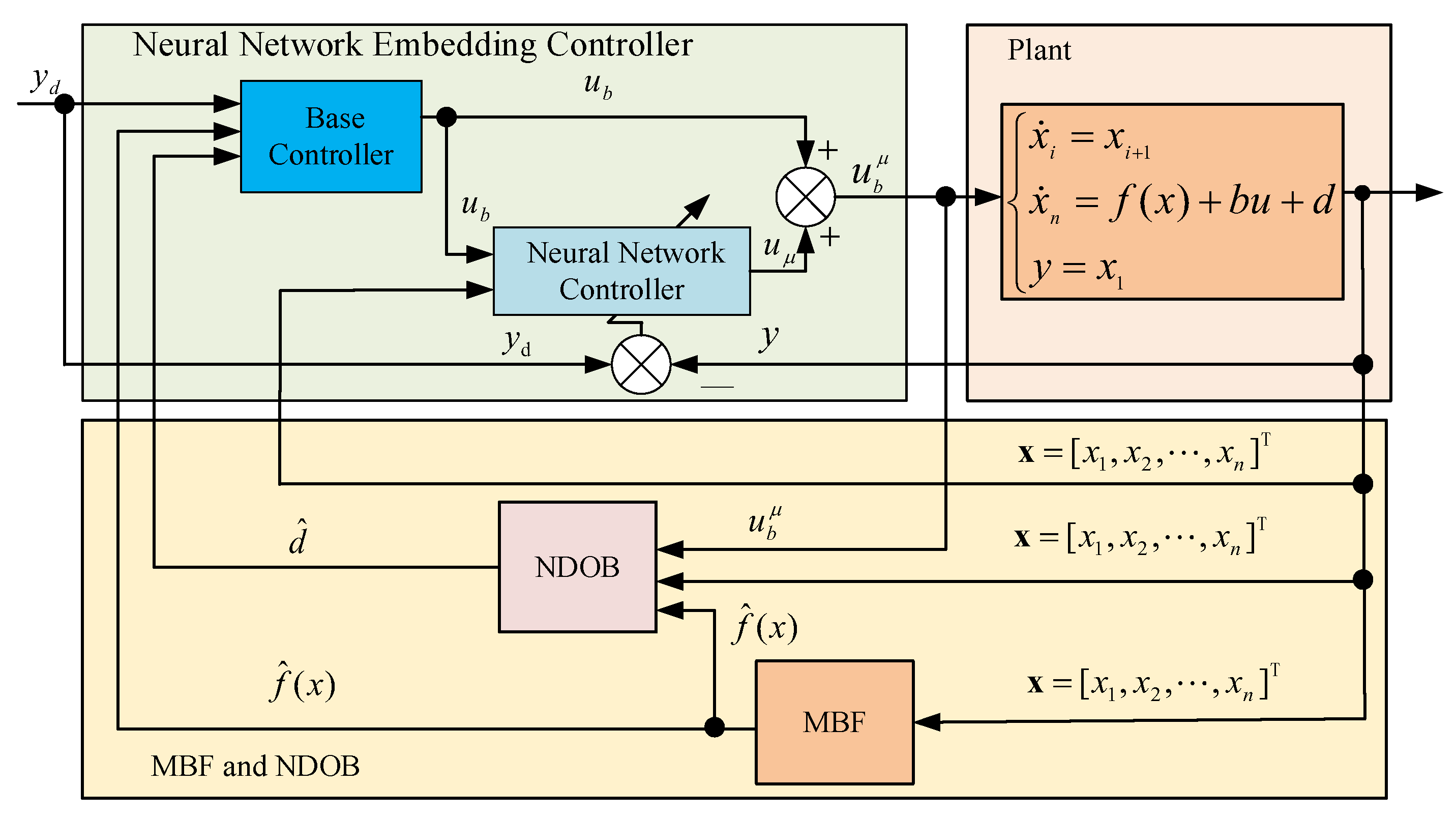
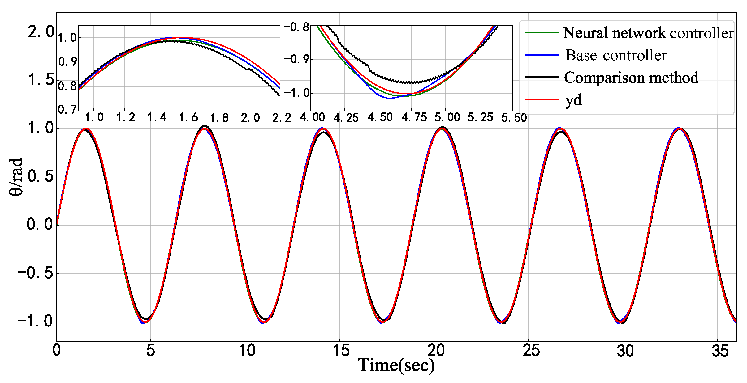
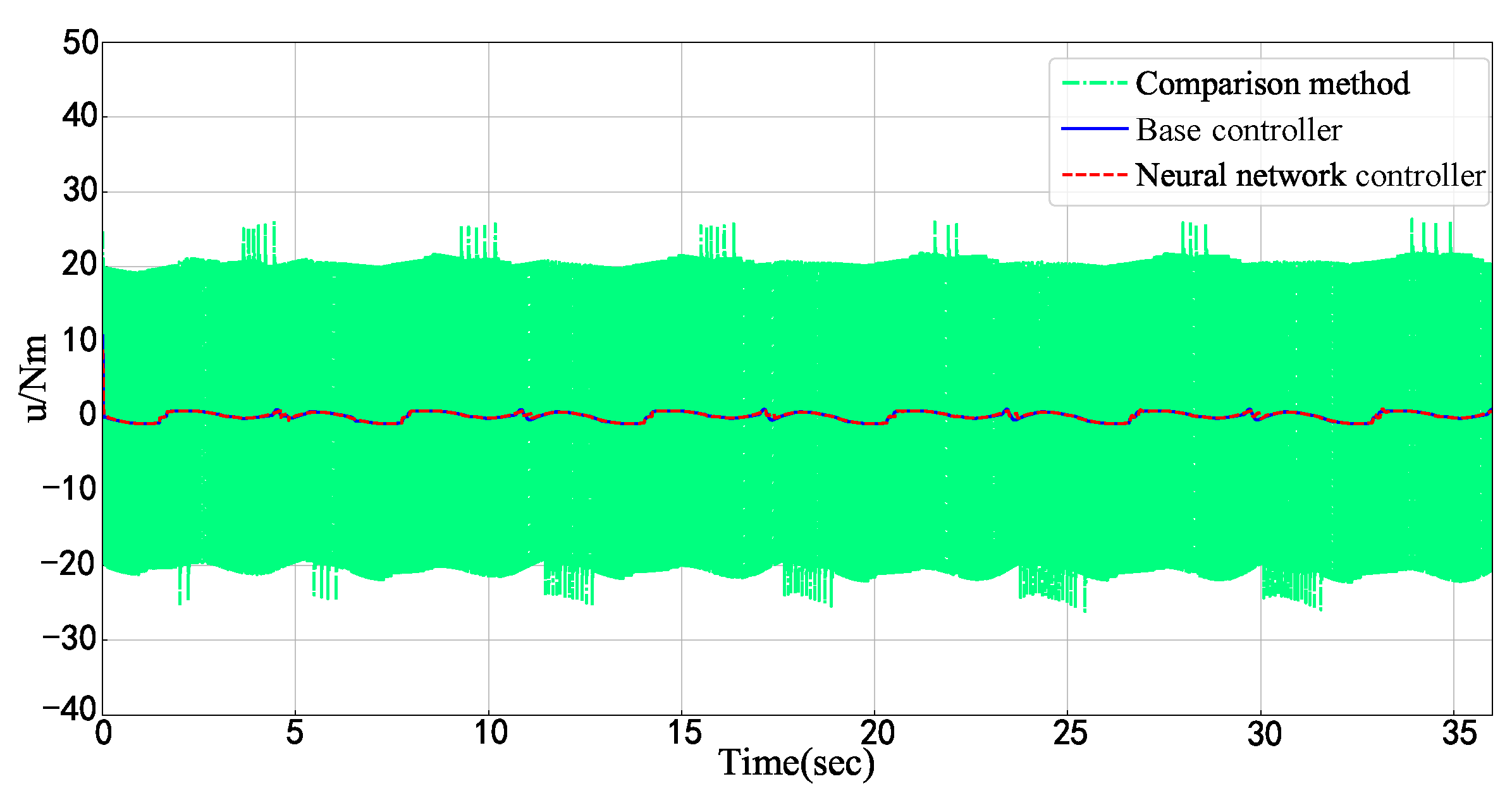
The proposed neural network embedding controller is able to improve control performance without impacting the Lyapunov stability of the base controller. In the practice, it can be regarded as a “hot plug” module, that is to say, it is capable of being embedded in any existing control scheme as long as the base controller is Lyapunov stable, and of optimizing the control performance by updating weight parameters according to a specific objective function.

This paper is organized as follows. First, Section 2 describes the controller and problems of nonlinear systems. The MBF and improved DOB are developed in Section 3, where the stability is also analyzed. Section 4 introduces neural network embedding and control performance optimization. Section 5 illustrates the effectiveness of the proposed approach through simulation experiment, while Section 6 carries the concluding remarks.

2. Problem Formulation and Preliminaries

2.1. System Statements

Consider a class of an n-order nonlinear system with uncertainty and disturbances as follows:

$$\left\{\begin{array}{cc}{\dot{x}}_i\hfill & =x_{i+1},i=1,\dots ,n-1\hfill \\ {\dot{x}}_n\hfill & =f\left(\mathit{x}\right)+bu+d\hfill \\ y\hfill & =x_1\hfill \end{array}\right.$$

(1)

where $x_i\in \mathrm{R}$ and $x_n\in \mathrm{R}$ are the states, n is the model order, $\mathit{x}={\left[x_1,x_2,\dots ,x_n\right]}^{\mathrm{T}}\in {\mathrm{R}}^{\mathrm{n}}$ is the state vector, $f\left(\mathit{x}\right)$ is the unknown smooth nonlinear functions in terms of $\mathit{x}$, $b>0$ represents an unknown control gain parameter of the system and it is the constant, $u\in \mathrm{R}$ is the control input, $d\in \mathrm{R}$ is the unknown external disturbance, and $y\in \mathrm{R}$ is the output of the system.

To achieve the control objective, the following assumptions widely existing in the related works (see [29,30]) are introduced for system (1).

Assumption A1. 

The unknown external disturbances d satisfy

$$\left|d\right|\le {\delta }_0$$

(2)

where ${\delta }_0$ is the unknown positive constant.

Assumption A2. 

The unknown control gain parameter b satisfies $b\le b_M$, where $b_M$ is a positive constant.

Assumption A3. 

The desired reference $y_d$ is a smooth and bounded function.

2.2. Controller Description

The block diagram of the control scheme in this paper is given in Figure 1, which is composed of neural network embedding controller, plant, MBF and nonlinear disturbance observer. As shown in Figure 1, to address the uncertainties and disturbances problems in the above system model (1), the MBF approximator and disturbance observer are employed to estimate and compensate, respectively. Then, the base controller is designed according to the MBF and disturbance observation. For the system performance optimization problem, the neural network embedded controller composed of the base controller and the neural network controller is used to optimize the system performance based on the condition that the base controller satisfies the Lyapunov stability to realize the trajectory tracking control of the control model.

3. Base Controller Design

3.1. Mixture Basic Functions (MBF) Approximator Design

This section aims is to solve the uncertainty problem in the considered system model (1), which exists the unknown form function $f\left(\mathit{x}\right)$. An effective method to address this problem is that the known form function is employed to approximate the unknown form function. The basis functions are usually applied as the nonlinear approximator:

$$f\left(\mathit{x}\right)={\mathit{\omega }}^{*T}\mathit{\phi }\left(\mathit{x}\right)+ϵ$$

(3)

where $f\left(\mathit{x}\right)$ is the unknown function to be approximated, and there exists an optimal weight vector ${\mathit{\omega }}^{*}\in \{\parallel \mathit{\omega }\parallel \le {\omega }_M\}$ to make the approximation error bounded, where ${\omega }_M$ is a positive constant, $\mathit{\phi }\left(\mathit{x}\right)$ is the basis function vector, and $ϵ$ is the approximation error.

At present, RBF is used as the basis function to approximate unknown nonlinear function. However, for the radial basis neurons, only when the input value is close to the center of the radial basis neurons can the radial basis neurons be activated. The Gaussian function ($G\left(x\right)=\exp \left(-\frac{{(x-\mu )}^2}{2{\sigma }^2}\right)$) is the most commonly used basis function of the RBF neural network, and its characteristics are shown in Figure 2. When the number of basis functions is fixed, the Gaussian basis function has value only in the bounded domain, and its value approaches zero when it is far away from the bounded domain as shown in Figure 2. This causes an inevitable problem that when the number of basic functions is fixed, RBF only can approximate the unknown nonlinear function in a bounded domain, out of which RBF could completely lose the approximation capability. Hence, we employ a MBF that consists of a polynomial function and trigonometric function as a function approximator to model the nonlinear function, and it has a strong global approximation ability. The combined data diagram of the polynomial function and trigonometric function is shown in Figure 3. As can be seen from Figure 3, compared with the RBF methods, the trigonometric functions and polynomial functions used in this paper can take non-zero values in any domains of independent variables and can achieve global approximation, that is, when the number of basis functions is fixed, MBF can approximate nonlinear functions in all domains by adjusting weights. There is no bounded domain restriction, so the MBF has the ability of global approximation to nonlinear functions.

We adopt the lemma as follows to prove the approximation ability of the mixture basis function.

Lemma 1 

(Weierstrass polynomial approximation theorem [31]). For any continuous function $f\left(x\right)\in C\left[a,b\right]$ and for any constants $\epsilon >0$, there exists an algebraic polynomial $p\left(x\right)$ satisfying the condition

$$\underset{a\le x\le b}{\sup }\left|f\left(x\right)-p\left(x\right)\right|\le \epsilon$$

(4)

where $p\left(x\right)=\sum _{i=0}^n{c}_i{x}^i$,$c_i,i=0,1,\dots ,n$ is the parameter, and n is the maximum order of $p\left(x\right)$.

Lemma 2 

(Trigonometric polynomials approximation theorem [31]). For any continuous periodic function $f\left(x\right)$, $x\in \mathrm{R}$ satisfying $f(x+2\pi )=f\left(x\right)$, there exists a polynomial of the form

$$q\left(x\right)=\frac{1}{2}{a}_0+\sum _{j=1}^n\left[a_{j}cos\left(jx\right)+b_{j}sin\left(jx\right)\right]$$

(5)

where $a_j,j=0,1,\dots ,n$ and $b_j,j=1,2,\dots ,n$ are real parameters, n is a finite integer, and $\delta >0$ such that the bound

$$\underset{x\in \mathrm{R}}{\sup }\left|f\left(x\right)-q\left(x\right)\right|\le \delta$$

(6)

Given polynomial and trigonometric basis function vectors ${\mathit{\phi }}_P$ and ${\mathit{\phi }}_{\mathit{Tr}}$, the mixture basis function can be expressed as

$${\phi }_M\left(\mathit{x}\right)={\mathit{\omega }}_P^T{\mathit{\phi }}_P\left(\mathit{x}\right)+{\mathit{\omega }}_{\mathit{Tr}}^T{\mathit{\phi }}_{\mathit{Tr}}\left(\mathit{x}\right)$$

(7)

where ${\mathit{\omega }}_P^T$ and ${\mathit{\omega }}_{\mathit{Tr}}^T$ are polynomial and trigonometric weight vectors, respectively. Therefore, we can define MBF weight and function vectors as ${\mathit{\omega }}^T=[{\mathit{\omega }}_P^T,{\mathit{\omega }}_{\mathit{Tr}}^T]$, ${\mathit{\phi }}_M\left(\mathit{x}\right)=[{\mathit{\phi }}_P,{\mathit{\phi }}_{\mathit{Tr}}]$, and an unknown nonlinear function can be approximated by MBF globally: $\widehat{f}\left(\mathit{x}\right)={\mathit{\omega }}^T{\mathit{\phi }}_M\left(\mathit{x}\right)$.

Remark 1. 

Theoretically, any function can be divided into two parts: periodic and nonperiodic. According to Lemmas 1 and 2, there exist the polynomial and the trigonometric function that are able to approximate two parts of the function, respectively. Hence, like RBF, MBF can approximate the arbitrary function. Meanwhile, the approximation of MBF is global rather than local as RBF.

3.2. Disturbance Observer Design

There are not only unknown nonlinear functions $f\left(\mathit{x}\right)$ but also unknown external disturbances d in system model (1). The nonlinear disturbance observer (NDOB) is mainly used to estimate and compensate for the disturbance, and a nonlinear disturbance observer is proposed in [32], described as

$$\left\{\begin{array}{c}\widehat{d}=z+g\left(\mathit{x}\right)\hfill \\ \dot{z}=-\mathit{l}\left(\mathit{x}\right){\mathit{g}}_2\left(\mathit{x}\right)z-\mathit{l}\left(\mathit{x}\right)\left({\mathit{g}}_2\left(\mathit{x}\right)g\left(\mathit{x}\right)+\mathit{f}\left(\mathit{x}\right)+{\mathit{g}}_1\left(\mathit{x}\right)u\right)\hfill \end{array}\right.$$

(8)

where $\widehat{d}$ denotes the estimation of the disturbance, z is the internal state of the nonlinear observer, $g\left(\mathit{x}\right)$ is a nonlinear function to be designed, and $\mathit{l}\left(\mathit{x}\right)$ is the nonlinear disturbance observer gain, and it should satisfy $\mathit{l}\left(\mathit{x}\right)=\partial g\left(\mathit{x}\right)/\partial \mathit{x}$. It is assumed that $\mathit{f}\left(\mathit{x}\right)$, ${\mathit{g}}_1\left(\mathit{x}\right)$ and ${\mathit{g}}_2\left(\mathit{x}\right)$ are the known smooth functions in terms of state $\mathit{x}$, and the NDOB needs to satisfy the assumption that the disturbance changes slowly or does not change; the meaning of this is $\dot{d}=0$.

According to Equation (8), a new disturbance observer is designed in this paper. Aiming at unknown smooth function $f\left(\mathit{x}\right)$ in nonlinear system Equation (1), the MBF is employed for approximation compensation and combined with Equations (8) and (3), and the improved disturbance observer is described as follows:

$$\left\{\begin{array}{c}\widehat{d}=f(z+g\left(\mathit{x}\right))\hfill \\ \dot{z}=-l\left(\mathit{x}\right)\widehat{d}-l\left(\mathit{x}\right)\left({\widehat{\mathit{\omega }}}^T{\mathit{\phi }}_M\left(\mathit{x}\right)+\widehat{b}u\right)\hfill \\ f(·)=\left\{\begin{array}{c}A,z+g\left(\mathit{x}\right)\ge A\hfill \\ z+g\left(\mathit{x}\right),-A<z+g\left(\mathit{x}\right)<A\hfill \\ -A,z+g\left(\mathit{x}\right)\le -A\hfill \end{array}\right.\hfill \end{array}\right.$$

(9)

where f is the bounded function, A is the constant to be designed, $\widehat{\mathit{\omega }}$ is the estimation of ${\mathit{\omega }}^{*}$, and $\widehat{b}$ is the estimation of b. So, we can obtain the equation as follows:

$$\left\{\begin{array}{c}\left|\widehat{d}\right|\le {\delta }_1\hfill \\ \tilde{d}=\widehat{d}-d\hfill \\ \left|\tilde{d}\right|\le {\delta }_2\hfill \end{array}\right.$$

(10)

where $\tilde{d}$ is the disturbance estimation error, and ${\delta }_1$ and ${\delta }_2$ are the unknown positive constants. From the above equation, it can be seen that the disturbance observer in this paper only needs to satisfy the condition of Equation (10), and the disturbance observer proposed in this paper only needs to ensure that the disturbance d is bounded. Hence, with the increased scope of application in practical applications, the disturbance rejection ability is guaranteed to improve the performance and robustness of the closed-loop system. The stability of the controller with the disturbance observer proposed in this paper is proved in Section 3.3.

3.3. Base Controller Design and Stability Analysis

The base controller based on the above MBF and improved disturbance observation is designed, and its stability is analyzed.

Theorem 1. 

For the system model in (1), the base controller is designed as

$$\left\{\begin{array}{c}{u}_b=\widehat{m}\left(k_1\dot{e}+{\ddot{y}}_{\mathrm{d}}-{\widehat{\mathit{\omega }}}^T{\mathit{\phi }}_M\left(\mathit{x}\right)-\widehat{d}+k_{2}s\right)\hfill \\ s=k_{1}e+\dot{e}\hfill \\ \dot{\widehat{m}}=s\left(k_1\dot{e}+{\ddot{y}}_{\mathrm{d}}-\widehat{\mathit{\omega }}{\mathit{\phi }}_M\left(\mathit{x}\right)-\widehat{d}+k_{2}s\right)-\alpha \widehat{m}\hfill \\ \dot{\widehat{\mathit{\omega }}}=-s{\mathit{\phi }}_M\left(\mathit{x}\right)-r\widehat{\mathit{\omega }}\hfill \end{array}\right.$$

(11)

Then, the closed-loop system is Lyapunov stable, where $m=\frac{1}{b}$, r, $k_1$, $k_2$ and α are the parameters to be designed, $e=y_d-y$.

Proof. 

The Lyapunov function candidate can be described as follows:

$$V_b=\frac{1}{2}{s}^2+\frac{1}{2}{∥\tilde{\mathit{\omega }}∥}^2+\frac{1}{2m}{\tilde{m}}^2$$

(12)

where $\tilde{\mathit{\omega }}=\widehat{\mathit{\omega }}-{\mathit{\omega }}^{*}$, $\tilde{m}=\widehat{m}-m$, and $\dot{\tilde{\mathit{\omega }}}=\dot{\widehat{\mathit{\omega }}}-{\dot{\mathit{\omega }}}^{*}$, $\dot{\tilde{m}}=\dot{\widehat{m}}-\dot{m}$.

Let $\nu =k_1\dot{e}+{\ddot{y}}_{\mathrm{d}}$; substituting Equations (3), (10) and (11), and the Lyapunov derivative of Equation (12) is given by

$$\begin{array}{cc}\hfill {\dot{V}}_b=& s(\nu -{\mathit{\omega }}^{*T}{\mathit{\phi }}_M\left(\mathit{x}\right)-ϵ-\frac{1}{m}{u}_b-d)\hfill \\ \hfill & +{\tilde{\mathit{\omega }}}^T(-s{\mathit{\phi }}_M\left(\mathit{x}\right)-r\widehat{\mathit{\omega }})\hfill \\ \hfill & +\frac{1}{m}\tilde{m}(s(\nu -{\widehat{\mathit{\omega }}}^T{\mathit{\phi }}_M\left(\mathit{x}\right)-\widehat{d}+k_{2}s)-\alpha \widehat{m})\hfill \\ \hfill =& s(\nu -({\widehat{\mathit{\omega }}}^T-{\tilde{\mathit{\omega }}}^T){\mathit{\phi }}_M\left(\mathit{x}\right)\hfill \\ \hfill & -\frac{1}{m}\left(\widehat{m}(\nu -{\widehat{\mathit{\omega }}}^T{\mathit{\phi }}_M\left(\mathit{x}\right)-\widehat{d}+k_{2}s)\right)\hfill \\ \hfill & -(\widehat{d}-\tilde{d}))+{\tilde{\mathit{\omega }}}^T(-s{\mathit{\phi }}_M\left(\mathit{x}\right)-r\widehat{\mathit{\omega }})\hfill \\ \hfill & +\frac{1}{m}\tilde{m}(s(\nu -{\widehat{\mathit{\omega }}}^T{\mathit{\phi }}_M\left(\mathit{x}\right)-\widehat{d}+ks)-\alpha \widehat{m})-sϵ\hfill \\ \hfill =& -k_2{s}^2-r{\tilde{\mathit{\omega }}}^T\widehat{\mathit{\omega }}-\frac{\alpha }{m}\widehat{m}\tilde{m}+s(\tilde{d}-ϵ)\hfill \\ \hfill =& -k_2{s}^2-r{\tilde{\mathit{\omega }}}^T\widehat{\mathit{\omega }}-\frac{\alpha }{m}\widehat{m}\tilde{m}+s\tilde{D}\hfill \end{array}$$

(13)

Now, using Young’s inequality [33], it follows that

$$\left\{\begin{array}{c}-r{\tilde{\mathit{\omega }}}^T\widehat{\mathit{\omega }}\le -\frac{r}{2}{∥\tilde{\mathit{\omega }}∥}^2+\frac{r}{2}{∥{\mathit{\omega }}^{*}∥}^2\hfill \\ s\tilde{D}\le \frac{1}{2}{s}^2+\frac{1}{2}{\tilde{D}}^2\hfill \\ -\frac{\alpha }{m}\tilde{m}\widehat{m}\le -\frac{\alpha }{2m}{\tilde{m}}^2+\frac{\alpha m}{2}\hfill \end{array}\right.$$

(14)

Thus, the following inequality can be obtained:

$$\begin{array}{cc}\hfill {\dot{V}}_b\le & -k_2{s}^2-\frac{r}{2}{∥\tilde{\mathit{\omega }}∥}^2+\frac{r}{2}{∥{\mathit{\omega }}^{*}∥}^2-\frac{\alpha }{2m}{\tilde{m}}^2\hfill \\ \hfill & +\frac{\alpha m}{2}+\frac{1}{2}{s}^2+\frac{1}{2}{\tilde{D}}^2\hfill \\ \hfill =& (\frac{1}{2}-k_2)s^2-\frac{1}{2}r{∥\tilde{\mathit{\omega }}∥}^2-\frac{\alpha }{2m}{\tilde{m}}^2\hfill \\ \hfill & +\frac{r}{2}{∥{\mathit{\omega }}^{*}∥}^2+\frac{1}{2}{\tilde{D}}^2+\frac{\alpha m}{2}\hfill \\ \hfill \le & -2c{V}_b+C_b^{*}\hfill \end{array}$$

(15)

where $\tilde{D}=\tilde{d}-ϵ$, c is the positive constant to be designed, $C_b^{*}=\frac{r}{2}{∥{\mathit{\omega }}^{*}∥}^2+\frac{1}{2}{\tilde{D}}^2+\frac{\alpha m}{2}$, and the design parameters satisfy

$$\left\{\begin{array}{c}\frac{1}{2}-k_2+c\le 0\hfill \\ -\frac{1}{2}r+c\le 0\hfill \\ -\frac{\alpha }{2m}+c\le 0\hfill \end{array}\right.$$

(16)

According to Assumptions 1 and 2, $\left|C_b^{*}\right|\le C_M^{*}$, where $C_M^{*}$ is a positive constant.

According to literature [34], let us express that ${\dot{V}}_b\left(t\right)=-2c{V}_b\left(t\right)+C_b^{*}+{\Delta }_V$, ${\Delta }_V\le 0$. Multiplying both sides by $e^{2ct}$, there is $d\left(e^{2ct}{V}_b\left(t\right)\right)/dt=e^{2ct}\left(C_b^{*}+{\Delta }_V\right)$. With the subsequent integration of both sides, we obtain

$$V_b\left(t\right)\le \frac{C_b^{*}}{2c}+\left(V_b\left(0\right)-\frac{C_b^{*}}{2c}\right)e^{-2ct}$$

(17)

All variables of $V_b\left(t\right)$ are uniformly ultimately bounded and stability can be obtained through the above proof.

This completes the proof of Theorem 1. □

4. Neural Network Embedding and Control Performance Optimization

4.1. Neural Network Embedding

A neural network embedding technology, which is based on the above base controller, is proposed to optimize the control performance. The additional neural network on the base controller is optimized by the loss function with the tracking error and the gradient descent method, which further reduces the tracking error and improves the control performance on the basis of the original controller. Firstly, the stability proof of the neural network control model embedding is given.

Theorem 2. 

For the system in (1), the neural network embedding controller is constructed as follows:

$$u_b^{\mu }=u_b+u_{\mu }(·\mid \mathit{\theta })$$

(18)

where $u_b$ is the base controller, $u_{\mu }(·\mid \mathit{\theta })$ is the neural network controller, and $\mathit{\theta }$ is all parameter vectors of the neural network. If satisfied, we have the following: (1) The base controller $u_b$ is uniformly ultimately bounded stability under Lyapunov function. (2) $\left|u_{\mu }(·\mid \mathit{\theta })\right|\le u_M$, where $u_M$ is positive. Then, $u_b^{\mu }$ is uniformly ultimately bounded stability under the Lyapunov function.

Proof. 

The Lyapunov function candidate and its derivative can be written as

$$\left\{\begin{array}{cc}\hfill & V=\frac{1}{2}{\xi }^2+\eta \hfill \\ \hfill & \dot{V}=\xi (M-f\left(\mathit{x}\right)-bu-d)+\psi \hfill \end{array}\right.$$

(19)

where $\xi$ and M are the functions in terms of state $\mathit{x}$ to be designed, and $\eta$ and $\psi$ are the other items with error.

The substitution of (18) into (19) yields

$$\begin{array}{cc}\hfill {\dot{V}}_{u_b^{\mu }}& =\xi \left(M-f\left(\mathit{x}\right)-d-b\left(u_b+u_{\mu }(·\mid \mathit{\theta })\right)\right)+\psi \hfill \\ \hfill & =\underset{V_b}{\underbrace{\xi \left(M-f\left(\mathit{x}\right)-d-b{u}_b\right)+\psi }}-\underset{V_{\mu }}{\underbrace{sb{u}_{\mu }(·\mid \mathit{\theta })}}\hfill \end{array}$$

(20)

According to conditions (1) and (2), using Young’s inequality to obtain

$$\begin{array}{cc}\hfill {\dot{V}}_{u_b^{\mu }}& \le -2c{V}_{\mathrm{b}}+C_{\mathrm{b}}^{*}-\xi b{u}_{\mu }(·\mid \mathit{\theta })\hfill \\ \hfill & \le -2c{V}_{\mathrm{b}}+C_{\mathrm{b}}^{*}+\frac{1}{2}{\xi }^2+\frac{1}{2}{b}^2{u_{\mu }}^2(·\mid \mathit{\theta })\hfill \\ \hfill & =-2c_{u_b^{\mu }}{V}_{u_b^{\mu }}+C_{u_b^{\mu }}^{*}\hfill \end{array}$$

(21)

where $c_{u_b^{\mu }}$ is the positive constant, $-2c_{u_b^{\mu }}{V}_{u_b^{\mu }}=-2c{V}_{\mathrm{b}}+\frac{1}{2}{\xi }^2$, $C_{u_b^{\mu }}^{*}=C_{\mathrm{b}}^{*}+\frac{1}{2}{b}^2{u_{\mu }}^2(·\mid \mathit{\theta })$. According to the above proof, the neural embedded network controller $u_b^{\mu }$ is uniformly ultimately bounded stability under Lyapunov function (19).This completes the proof of Theorem 2. □

Remark 2. 

It can be seen from Theorem 2 that there is no limit to the input and form of the neural network, which thus allows user design on the basis of the specific application situation. Hence, a neural network model that is relatively universal in form is described in this paper.

In this paper, the structure of neural network of controller $u_{\mu }$ is offered, that is, a three-layer multilayer perceptron (MLP). The values of the input layer are respectively transmitted to the hidden layer through network calculation and then transmitted to the output layer in the same way. The relationship from input $\mathit{X}$ to neural network controller $u_{\mu }$ is as follows:

$$\left\{\begin{array}{c}\mathit{H}={\mathit{W}}^{\mathit{T}}\mathit{X}\hfill \\ \mathit{Y}={\mathbf{G}}^{\mathit{T}}\mathbf{\Gamma }\left(\mathit{H}\right)\hfill \\ u_{\mu }=\vartheta \left(\mathit{Y}\right)\hfill \end{array}\right.$$

(22)

where $\mathit{W}$ and $\mathbf{G}$ are the connection weight matrices of the the input layer to the hidden layer and hidden layer to the output layer, respectively, $\mathit{H}$ is the intermediate vector, and $\mathbf{\Gamma }$ is the activation function for the hidden and output layers. The Sigmoid function is used as the activation function, and some optimization algorithms, such as stochastic gradient descent (SGD) or adamax, can be used to tune the parameters of $\mathit{W}$ and $\mathbf{G}$. The output value $\mathit{Y}$ is obtained in the output layer, and then the improved tanh function $\vartheta \left(x\right)=\kappa \frac{e^x-e^{-x}}{e^x+e^{-x}}$ is used as the bounded function of the constrained neural network. $\kappa$ is the gain coefficient, which is a key parameter to ensure that the output of neural network satisfies the Theorem 2 condition, and the neural network controller $u_{\mu }=\vartheta \left(\mathit{Y}\right)$ is obtained.

4.2. Control Performance Optimization

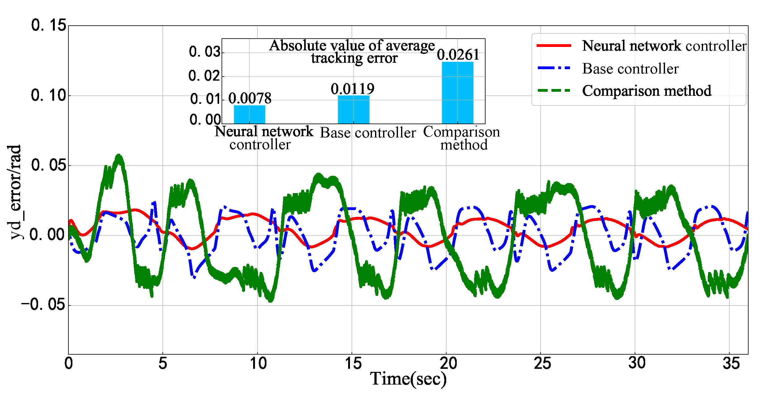
Based on the stable embedding of the above neural network, the embedding controller enables optimized control performance by adjusting the parameters of the neural network based on some learning algorithm. Due to the automatic derivation technology and optimization method in deep learning, the performance optimization of neural network learning controller can be reduced to the design of the control performance objective function. The objective function of the neural network is designed:

$$\mathcal{L}\left(\theta \right)={\left(y-y_d\right)}^2$$

(23)

where y is the system output, and $y_d$ is the desired trajectory. Due to there being no specific requirement for the form of the neural network in Theorem 2, the optimization algorithm based on gradient as a more general method is considered.

The gradient of $\mathcal{L}$ to $\mathit{\theta }$ in Equation (23) can be obtained:

$$\frac{\partial \mathcal{L}}{\partial \mathit{\theta }}=2(y-y_d)\frac{\partial y}{\partial u_{\mathrm{b}}^{\mu }}\frac{\partial u_{\mathrm{b}}^{\mu }}{\partial \mu }\frac{\partial \mu }{\partial \mathit{\theta }}$$

(24)

Due to there being unknown nonlinear functions and disturbances in system (1), it is difficult to solve or identify $\frac{\partial y}{\partial u_b^{\mu }}$ directly.

By observing Equation (1), we find a feature as follows:

$$\frac{\partial y}{\partial u_b^{\mu }}\propto \iota$$

(25)

where $\iota$ is constant. In the process of optimizing the neural network based on the gradient method, learning rate $\lambda$ is usually needed to adjust the updating speed of the network weight, so $\iota$ can be converted into learning law $\lambda$:

$${\mathit{\theta }}_k={\mathit{\theta }}_{k-1}-\lambda \frac{\partial \mathcal{L}}{\partial {\theta }_{k-1}}$$

(26)

According to Equation (26), a loss function ${\mathcal{L}}_{\lambda }$ equivalent to Equation (23) can be established:

$$L_{\lambda }\left(\theta \right)=\left(y-y_d\right){\rho }_{\lambda }{u}_b^{\mu }$$

(27)

where ${\rho }_{\lambda }$ is a tunable positive constant.

Therefore, the control performance improvement be realized by constructing the objective function with the tracking error as the optimization term and using the gradient descent method.

To sum up, the whole process with respect to the control scheme of this paper is shown in

Table 1. Control scheme of the proposed method.

Control Flow
Nonlinear Function Approximation:	$\widehat{f}\left(\mathit{x}\right)={\widehat{\mathit{\omega }}}^T{\mathit{\phi }}_M\left(\mathit{x}\right)$
Disturbance Estimation:	$\widehat{d}=f(z+g\left(\mathit{x}\right))$
Base Controller:	$u_b=\widehat{m}\left(k_1\dot{e}+{\ddot{y}}_{\mathrm{d}}-{\widehat{\mathit{\omega }}}^T{\mathit{\phi }}_M\left(\mathit{x}\right)-\widehat{d}+k_{2}s\right)$
Neural Network Embedding Controller:	$u_b^{\mu }=u_b+u_{\mu }(·\mid \mathit{\theta })$
Parameters Update:	$\left\{\begin{array}{c}\dot{z}=-l\left(\mathit{x}\right)\widehat{d}-l\left(\mathit{x}\right)\left({\widehat{\mathit{\omega }}}^T{\mathit{\phi }}_M\left(\mathit{x}\right)+\widehat{b}u\right)\hfill \\ f(·)=\left\{\begin{array}{c}A,z+g\left(\mathit{x}\right)\ge A\hfill \\ z+g\left(\mathit{x}\right),-A<z+g\left(\mathit{x}\right)<A\hfill \\ -A,z+g\left(\mathit{x}\right)\le -A\hfill \end{array}\right.\hfill \end{array}\right.$
	$\dot{\widehat{m}}=s\left(k_1\dot{e}+{\ddot{y}}_{\mathrm{d}}-\widehat{\mathit{\omega }}{\mathit{\phi }}_M\left(\mathit{x}\right)-\widehat{d}+k_{2}s\right)-\alpha \widehat{m}$
	$\dot{\widehat{\mathit{\omega }}}=-s{\mathit{\phi }}_M\left(\mathit{x}\right)-r\widehat{\mathit{\omega }}$
	${\mathit{\theta }}_k={\mathit{\theta }}_{k-1}-\lambda \frac{\partial \mathcal{L}}{\partial {\mathit{\theta }}_{k-1}}$

.

5. Simulations

In this section, some simulation experiments are carried out by using the nonlinear numerical model and motor model to verify the effectiveness of our method. Example 1 verifies the global approximation ability of MBF to unknown nonlinear functions. Example 2 verifies the compensation ability of the improved disturbance observer to unknown disturbances. Example 3 embeds the neural network controller into the base controller to verify the optimization ability of the neural network controller. All simulations are based on the Python framework, in which Pytorch is used as the neural network library. All of the codes for our methods will be released, see https://github.com/SheldonCooper233/Mixture-Basis-Function-Approximation-and-Neural-Network-Embedding-Control (accessed on 17 May 2023).

5.1. Numerical Model Examples

Example 1. 

In this example, we consider the approximation performance of MBF. We consider a second-order nonlinear system with trigonometric functions, polynomial functions, and dead zones. Using MBF and RBF [8] to perform comparative experiments, we verify the global approximation ability of MBF for unknown nonlinear functions. The second-order model is as follows:

$$\left\{\begin{array}{c}{\dot{x}}_1=x_2\hfill \\ {\dot{x}}_2=f(x_1,x_2)+bu\hfill \\ f=\left\{\begin{array}{c}0,\left|x_1\right|<{\delta }^{*}\mathrm{or}\left|x_2\right|<{\delta }^{*}\\ l_1{x}_{1}cos\left(x_1\right)+l_2{x}_{2}sin\left(x_2\right)+l_3{x}_1^2+l_4{x}_2^2\end{array}\right.\hfill \end{array}\right.$$

(28)

where ${\delta }^{*}=0.1$, $l_1=10$, $l_2=5$, $l_3=2$, $l_4=3$, $b=0.5$.

According to Equation (11), the base controller is established, where $k_1=10$, $k_2=5$, $\alpha =0.3$, $r=0.05$, and according to Lemma 1 and 2, the MBF is designed as follows:

$$\begin{array}{cc}\hfill {\mathit{\phi }}_M\left(x\right)=& \left[1,l_5\mathit{sin}\left(x_1\right),l_5\mathit{sin}\left(x_2\right)\right.\hfill \\ \hfill & l_5\mathit{cos}\left(x_1\right),l_5\mathit{cos}\left(x_2\right),l_5\mathit{sin}\left(2x_1\right)\hfill \\ \hfill & l_5\mathit{cos}\left(2x_1\right),l_5\mathit{sin}\left(2x_2\right),l_5\mathit{cos}\left(2x_2\right)\hfill \\ \hfill & \left.l_6{x}_1,l_6{x}_2,l_6{x}_1^2,l_6{x}_2^2,l_6{x}_1^3,l_6{x}_2^3\right]\hfill \end{array}$$

(29)

where $l_5=0.7$, $l_6=0.18$. Two groups of simulations are used to verify the global approximation advantage of the MBF algorithm. The simulation condition is as follows: in the RBF, there are 100 nodes with the center placed on [−3, 3] and the width of the Gaussian functions is ${\sigma }^2=1$, while the remaining parameters and MBF parameters remain the same. The desired expected trajectories are $y_d=sin\left(t\right)$ and $y_d=5sin\left(t\right)$, respectively, that is, the range of values for $x_1$, $x_2$ is [−1, 1] and [−5, 5], respectively.

Figure 4, Figure 5, Figure 6, Figure 7, Figure 8, Figure 9, Figure 10 and Figure 11 show the simulation comparison results of $y_d=sin\left(t\right)$ and $y_d=5sin\left(t\right)$ for two control methods. Figure 4, Figure 5, Figure 6, Figure 7, Figure 8, Figure 9, Figure 10 and Figure 11 show the following results: (1) All the two methods can achieve the trajectory tracking of the system with higher accuracy. As can be seen from Figure 4 and Figure 8, the RBF method has a higher output value than expected at the peak and a lower output than expected at the trough. When the value range of $x_1$ and $x_2$ is far from the central point of RBF, the tracking performance is degraded due to its local approximation characteristics, while the MBF can achieve fast tracking and be closer to the expected value. (2) As can be seen from Figure 7 and Figure 11, the absolute value of the average approximation error of RBF is greater than the absolute value of the average approximation error of MBF for the nonlinear functions, and the approximation error of RBF at the initial time is very large in Figure 11 due to the RBF being a function of the local approximation. Because when the range of independent variables is far from the central point of RBF, the value of the RBF Gaussian basis function approaches zero, resulting in a significant decrease in the approximation effect or even loss of approximation ability. (3) As can be seen from Figure 5 and Figure 9, the control output amplitudes of the two methods are generally consistent. In Figure 9, the initial time control input becomes larger due to the local approximation characteristic of RBF. As shown from Figure 6 and Figure 10, the tracking error ranking is still the classical RBF > MBF. As mentioned above, for a nonlinear second-order system with trigonometric functions and dead zones, the effect of this article method is better than the classic RBF adaptive method.

Remark 3. 

As these results mentioned above, it can be concluded that MBF has higher approximation accuracy for a relatively complex nonlinear function compared with the classical RBF methods, which results in a superior tracking error performance to the compared method.

Example 2. 

The objective of this example lies in validating the disturbance estimation performance of our methods. We consider a second-order nonlinear system with nonlinear function and random disturbance. We use MBF and DOB of our designed to compare with RBF and sliding-mode disturbance observer (SMDOB) [16]. The purpose of the experiment is to verify the compensation ability of the improved disturbance observer to disturbance. The second-order model is as follows:

$$\left\{\begin{array}{c}{\dot{x}}_1=x_2\hfill \\ {\dot{x}}_2=f(x_1,x_2)+bu+d\hfill \\ f=exp(-\frac{{(x_1-{\varsigma }_1)}^2}{2{\varpi }_1^2})+exp(-\frac{{(x_2-{\varsigma }_2)}^2}{2{\varpi }_2^2})+x_1+x_2\hfill \end{array}\right.$$

(30)

where ${\varsigma }_1=1$, ${\varpi }_1=1$, ${\varsigma }_2=1$, ${\varpi }_2=1$, $b=2$.

According to Equation (11), the base controller is established, where $k_1=20$, $k_2=5$, $\alpha =0.2$, $r=0.1$, and the MBF is designed as Equation (29), where $l_5=0.4$, $l_6=0.5$.

In Example 2, the following disturbance is added to the above model:

$$d\left(t\right)=G_{d}sin\left({\omega }_{d}t\right)+{\xi }_d\left(t\right)$$

(31)

where $G_d=3$, ${\omega }_d=2$, ${\xi }_d$ is a random number of [−5, 5], ${\xi }_d$ is the same in the two methods, and the disturbance observer gain $l=6$, $A=4$. The performance of the SDOB tends to be optimized, and the parameters are set as $k_c=2.1$, $A=10$, $C=5$, $g=0.5$, $\phi =5.2$.

Figure 12, Figure 13 and Figure 14 shows the simulation comparison results of the two control methods of $y_d=sin\left(t\right)$. Figure 12, Figure 13 and Figure 14shows the results: (1) Under the condition of disturbance in Equation (31), all two methods realize the stable tracking of $y_d$, and the absolute value of the average tracking error of the SDOB is greater than that of the disturbance observer (DOB) in this paper. (2) For the approximation ability of disturbance, the absolute value of the mean approximation error of the SDOB is greater than that of the DOB in this paper. The reason is that the SDOB has multiple parameters, while the DOB designed in this paper has only one parameter and is easy to adjust. (3) The amplitude of the control input of SDOB is larger than that of DOB. The reason is that the compensation effect of SDOB to disturbance is poor under strong disturbance, and the influence of disturbance is suppressed by increasing the control input and the tracking error ranking is the SMDOB > DOB. This shows that under the strong disturbance condition, the compensation and suppression ability of the DOB in this paper is better than the SDOB.

Remark 4. 

As these results mentioned above, it can be concluded that even though the precondition is relaxed, the improved DOB still has superior disturbance estimation performance compared with classical methods. Hence, improved DOB could have more benefits in the practice.

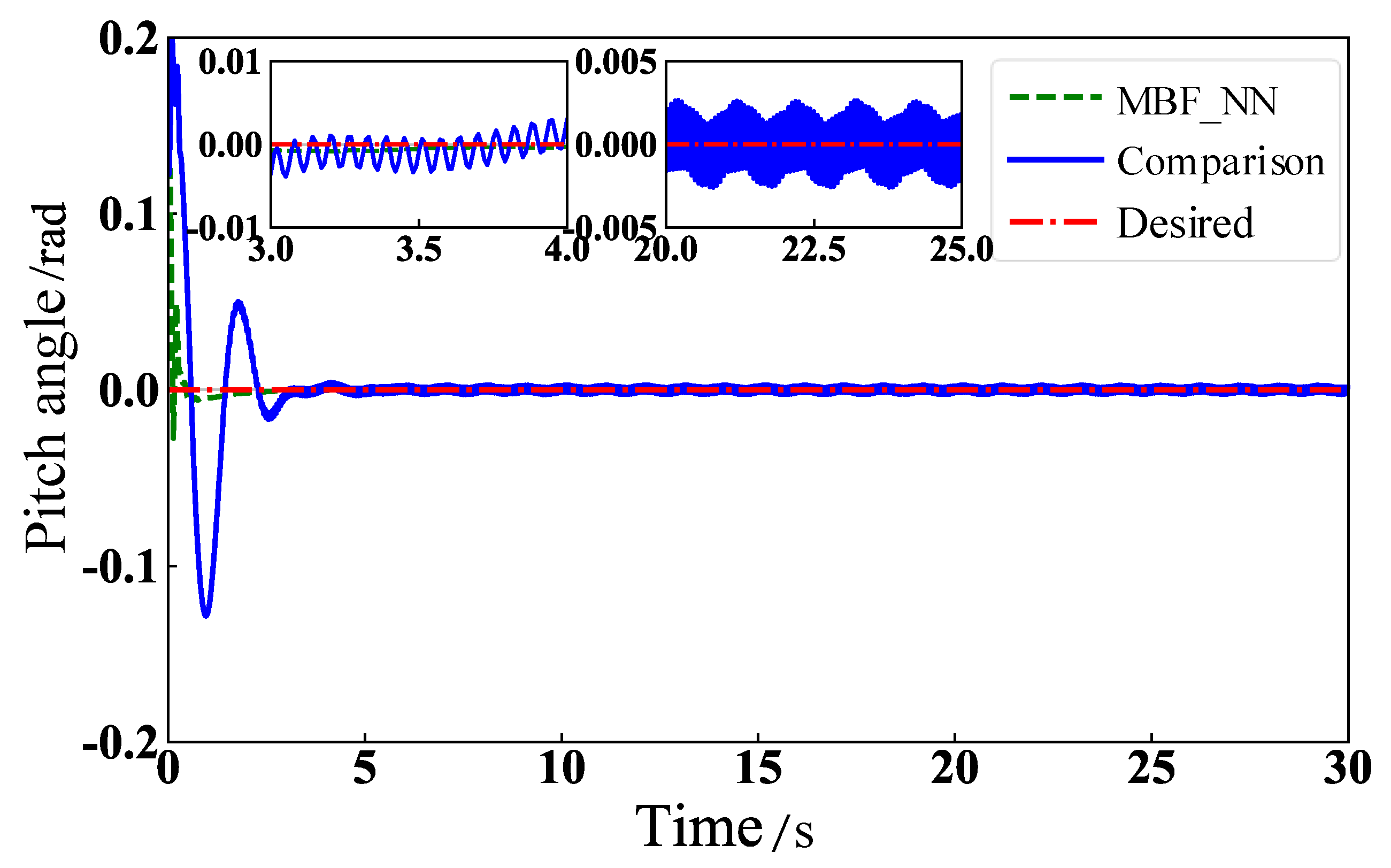
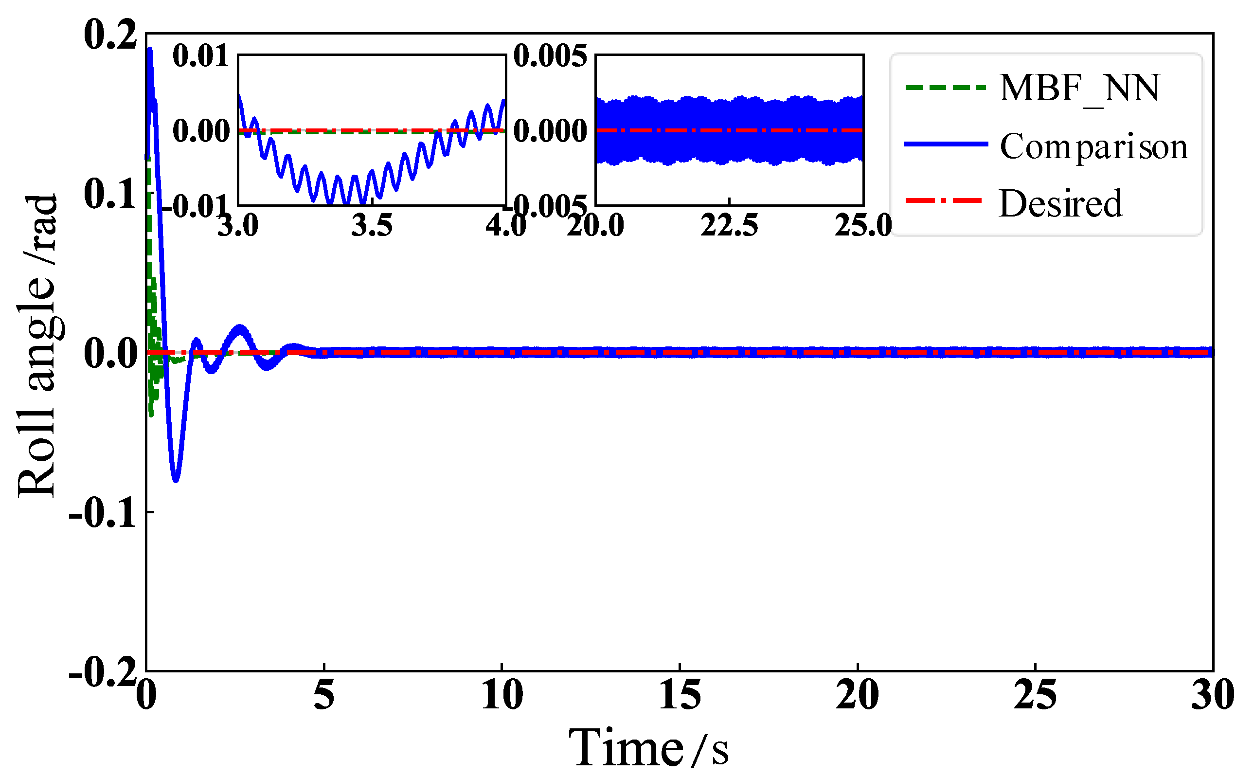
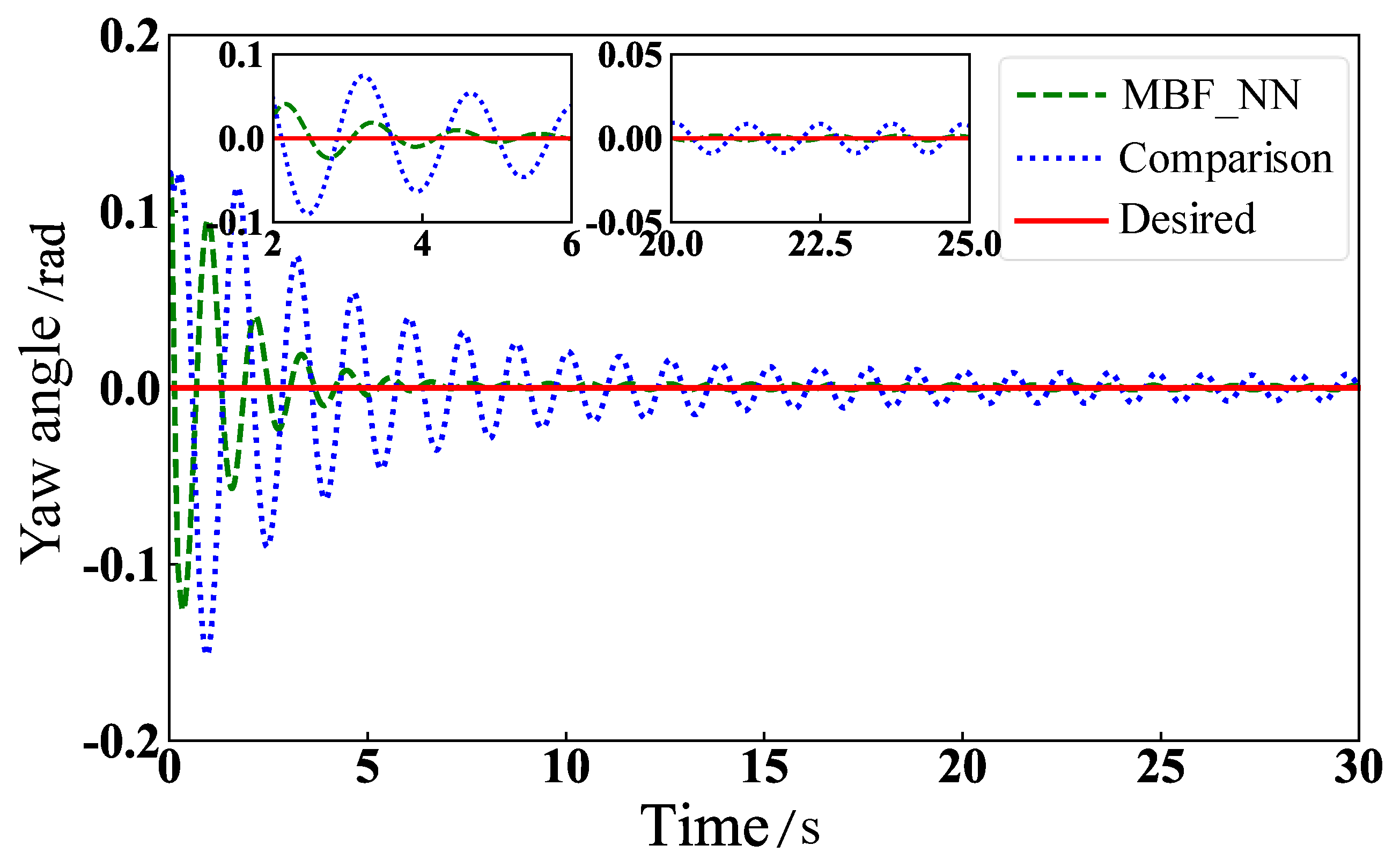
5.2. Physical Model Simulation

To further validate the effectiveness of the proposed scheme, a motor system model is considered in this section. The neural network optimization method is added to the base controller to test the actual motor model to verify the performance of the neural network embedding controller. The comparison algorithms are as follows: (1) Base controller with MBF and improved DOB. (2) The neural network embedding controller. (3) Comparison method [35].

Remark 5. 

In this example, we focus on the control performance with respect to the proposed neural network embedding method. Consider a motor torque control model of exponential friction characteristics, as follows:

$$\left\{\begin{array}{c}\dot{\theta }=\omega \hfill \\ \dot{\omega }=f_M(\theta ,\omega )+\frac{K+K_{\theta }}{T}\tau \hfill \\ f_M(\theta ,\omega )=\left\{\begin{array}{cc}0,\left|\theta \right|<{\sigma }^{*}\mathrm{or}\left|\omega \right|<{\sigma }^{*}& \\ -\frac{1}{T}\omega +\frac{K+K_{\theta }}{T}{T}_f\end{array}\right.\hfill \\ T_f=T_{c}sgn\left(\omega \right)+(T_s+T_c)e^{-\alpha \left|\omega \right|}sgn\left(\omega \right)\hfill \end{array}\right.$$

(32)

where θ is the motor rotation angle (rad), ω is the angular velocity (rad/s), τ is the control input (N·m), $f_M$ is the nonlinear term, $T_f$ is the friction force, and the model parameters are $K=2.97$, $K_{\theta }=0.25$, $T=0.632$, $T_c=0.2$ N·m, $T_s=0.3$ N·m, and $\alpha =1.0$. Applied as (31) disturbance, $G_d=3.0$, ${\omega }_d=2.0$, and the disturbance observer gain $l=0.1$, $A=4$.

The base controller is designed as (11), where $k_1=10$, $k_2=15$, $\alpha =0.1$, $r=0.5$, and the MBF is designed as (29), where $l_5=2.5$ and $l_6=1.2$. The performance of the comparison method tends to be optimized, the parameters are set as $c=10$ and $\eta =15$, and the value range of the central point of the RBF network is [−5, 5]; see reference [35] for other parameters. Considering the control rate of motor system, we utilize the shallow network.

According to Equation (22), the input vector of the input layer is set by $\mathit{X}={\left[\theta ,{\theta }_d,\tau \right]}^T$, where $\theta$ is the motor angle, ${\theta }_d$ is the motor desired angle, $\tau$ is the control torque, $\mathit{W}$ and $\mathbf{G}$ dimensions are $3\times 90$, $90\times 1$, $\kappa =3$, and the optimization algorithm is set as SGD with the learning rate $\lambda =0.001$.

Our control objective is to render the system output y following a given desired trajectory $y_d=sin\left(t\right)$. Figure 15, Figure 16 and Figure 17 show the comparison of the control effects of the three methods. (1) Figure 15 shows that the method in this paper can quickly realize tracking in the initial stage, but the comparison method has a larger error than the method in this paper in the initial stage (see the first peak and trough). (2) Figure 16 shows that due to the embedding of the neural network controller, the performance of the basic controller is optimized to some extent, and the amplitude of the control input of the contrast method is very large. (3) Figure 17 shows that the tracking error of the method in this paper is generally lower than that of the comparison method. After embedding the neural network controller, the tracking error is smaller than that of the base controller. The absolute value of the average tracking error ranking is still comparison method > base controller > neural network embedding controller.

The maximum error (max$\left|e\right|$), average error (mean$\left|e\right|$), maximum control output (max$\left|u\right|$), and average control output (mean$\left|u\right|$) of the three methods are compared as shown in

Table 2. The comparison for control statistical indicators of three methods in Example 3.

Methods	Max$\left|\mathit{e}\right|$	Mean$\left|\mathit{e}\right|$	Max$\left|\mathit{u}\right|$	Mean$\left|\mathit{u}\right|$
Comparison method	$0.05750$	$0.0261$	$26.3265$	$20.4733$
Base controller	$0.02525$	$0.0119$	$10.7119$	$0.4626$
Neural network controller	$0.01829$	$0.0078$	$8.8509$	$0.4495$

.

According to Table 2, the maximum error, the maximum control output, the average error, and the average control output of the neural network embedding method are all minimum values. It can be concluded that the control effect of the method in this paper is superior to the comparison method for Example 3 as a whole. Due to the use of the neural network controller, the control performance of the neural network embedding controller is greatly improved compared with the base controller. The results of performance optimization fully prove the rationality and effectiveness of the gradient optimization method proposed in the fourth section.

Remark 6. 

As these results mentioned above, it can be concluded that the control performance results, such as output tracking error and input amplitude, are further improved by embedding the neural network controller to the base controller and by tuning the weight parameters of the network in the control process.

On the basis of the results of the three examples, it is concluded that compared with the existing and popular methods for the problems of function approximation and disturbance estimation, the MBF and improved DOB we proposed have superior performance. The neural network embedding controller can improve the system control performance.

6. Virtual Experiments

In this section, a fully actuated vehicle is employed as the virtual experiment object for attitude control to confirm the efficiency of the method in practical applications. The vehicle has a load suspended below it, and as it takes off, the rope carrying the load will wobble, owing to gravity and inertia, causing a disturbance to the vehicle [36]. The fully actuated drive vehicle virtual experiment platform is shown in Figure 18.

To avoid potential safety and equipment damage issues that could arise in actual flight, this research simulates the experimental tests of an fully actuated vehicle using the CoppeliaSim software 4.1.0. The academic community has gradually come to recognize and use CoppeliaSim as an experimental instrument since it offers advantages over alternative simulation testing methods in terms of safety and efficiency, cheap cost, and better fit with the actual system [37,38,39]. Therefore, CoppeliaSim is chosen as the virtual experimental platform to verify the practical effectiveness of the algorithm in this paper. The control period of the virtual experiment is set to 0.01s, the physics engine is selected as “Bullet 2.78” and the accuracy is set to “highest accuracy”. The control algorithm is written in Python and communicates with CoppeliaSim via the application programming interface (API) provided by CoppeliaSim for remote synchronization.

Model the vehicle platform dynamics according to the Euler equation:

$$\{\begin{array}{c}\dot{\mathbf{\Omega }}=\mathit{J}\mathbf{\Theta }\hfill \\ \mathit{I}\dot{\mathbf{\Theta }}+\mathbf{\Theta }\times \mathit{I}\mathbf{\Theta }={\mathit{\tau }}_{\mathrm{fp}}+{\mathit{\tau }}_{\mathrm{h}}+{\mathit{d}}_{\mathrm{ext}}\hfill \end{array}$$

(33)

where $\mathbf{\Omega }={\left[\varphi ,\theta ,\phi \right]}^T$ is the vehicle attitude angle, $\mathbf{\Theta }={[\dot{\varphi },\dot{\theta },\dot{\phi }]}^T$ is the vehicle attitude angular velocity, $\mathit{J}$ is the Jacobian matrix, $\mathit{I}=diag[I_x,I_y,I_z]$ is the rotational inertia matrix,${\mathit{\tau }}_{\mathrm{fp}}$ is the sum of the moments of the flight platform, ${\mathit{\tau }}_{\mathrm{h}}$ represents the moment of the suspended load acting on the flight platform, and ${\mathit{d}}_{\mathrm{ext}}$ is other external disturbances. In practice, it is difficult to measure $\mathit{I}$ accurately; therefore, for the control side, the vehicle specific model parameters and perturbations are unknown and belong to the system model with unknown dynamics and perturbations without loss of generality [40], and the vehicle attitude system model is collapsed into the following form according to Equation (33):

$$\{\begin{array}{c}\dot{\mathbf{\Omega }}=\mathit{J}\mathbf{\Theta }\hfill \\ \dot{\mathbf{\Theta }}=\mathit{\beta }\mathit{\tau }+\mathit{F}+\mathit{d}\hfill \end{array}$$

(34)

where, $\mathit{F}$ denotes the unknown non-linear term in the system model, $\mathit{\beta }={\mathit{I}}^{-1}$, $\mathit{\tau }$ denotes the control moment, and $\mathit{d}$ denotes the unknown disturbance.

The virtual experiment is conducted using the methodology described in the literature [41] (hereinafter referred to as the “comparison method”), and the base controller of this paper is established in accordance with Equation (11) with parameters $k_1=30,k_2=200,\alpha =3,r=2$. The hybrid basis function is designed in accordance with Equation (29) with parameters $l_5=8,l_6=3$, and the neural network controller structure is designed in accordance with Example 3, where the input vector $\mathit{X}={[\mathbf{\Omega },{\mathbf{\Omega }}_d,\mathit{\tau }]}^T$, $\mathbf{\Omega }$ is the actual attitude angle during vehicle control, ${\mathbf{\Omega }}_d$ is the desired attitude angle and $\mathit{\tau }$ is the control moment. The Sigmoid function is used for the activation function, and $\mathit{W}$ and $\mathbf{G}$ dimensions are $3\times 16$, $16\times 1$, $\kappa =10$. The optimization algorithm is set to Adamax with the learning rate $\lambda =0.003$. After the output value Y is obtained from the output layer, the neural network controller $u_{\mu }=\vartheta \left(Y\right)$ is obtained by a bounded function $\vartheta$, and the gain coefficient of the bounded function $\kappa =10$ is taken. The initial position of the vehicle is [0 m, 0 m, 1 m], the desired position is [1 m, 1 m, 2 m], the initial Euler angle and the desired Euler angle are both $[0^{\circ },0^{\circ },0^{\circ }]$, the flight platform mass of the vehicle is 3.6 kg and the load mass is 1 kg.

Figure 19, Figure 20, Figure 21, Figure 22 and Figure 23 compare the attitude control effect of the method used in this paper (in the diagram, it is called MBF-NN) and the comparison method (in the diagram, it is called comparison) in the virtual flight experiment. The results are analyzed as follows: (1) From Figure 19, Figure 20 and Figure 21, it can be seen that both control schemes converge to the desired signal due to the good compensation effect of this paper’s method for unknown dynamics and perturbations and the optimization effect of the neural network on the underlying controller, which makes the response of this paper’s method faster and better tracking than the comparison method. (2) It is shown in Figure 22 that this approach’s control performance is superior to the comparison method due to the neural network’s embedding. (3) From Figure 23, it can be seen that the method in this paper has a smaller average tracking error compared to the comparison method.

Based on the results of the virtual experiment, it is clear that our method has superior control performance while controlling the attitude of a vehicle with unknown model and disturbance, thus verifying the effectiveness of this method in applications with respect to actual physics systems.

Therefore, simulations and virtual experiments validate the advantages with respect to the control scheme proposed in this article at nonlinear approximation, disturbance estimation and performance improvements for nonlinear system control.

7. Conclusions

This paper draws the following conclusions through the analysis and test results:

(1) Compared with the RBF, the MBF approximator proposed in this paper has a superior approximation effect for nonlinear functions due to its global approximation ability. (2) The improved DOB has a wider range of application, does require the precondition of slow change with respect to disturbance, and still has superior estimation performance in the case of random strong disturbance. (3) The proposed neural network embedding controller can improve control performance under Lyapunov stability and thus can be regarded as a “hot-plug” module with respect to the original base controller. Meanwhile, it does not have to restrict the type of neural network, and the user thus could design a specific structure of the network, such as some deep neural networks, according to the features of the control task.

In future works, there are some issues left to be investigated, which are as follows: (1) Introduce other control performance indices to improve the optimization objective function and design new neural network structures. (2) Extend the application domain to that between multiple inputs and multiple outputs systems. (3) Apply the control algorithm to practical experiments.

References

1. Yeam, T.I.; Lee, D.C. Design of sliding-mode speed controller with active damping control for single-inverter dual-PMSM drive systems. IEEE Trans. Power Electron. 2021, 36, 5794–5801. [Google Scholar] [CrossRef]
2. Ding, L.; Liu, C.; Liu, X.; Zheng, X.; Wu, H. Kinematic stability analysis of the tethered unmanned aerial vehicle quadrotor during take-off and landing. Chin. J. Sci. Instrum. 2020, 41, 70–78. [Google Scholar]
3. Hu, Y.; Benallegue, M.; Venture, G.; Yoshida, E. Interact with me: An exploratory study on interaction factors for active physical human-robot interaction. IEEE Robot. Autom. Lett. 2020, 5, 6764–6771. [Google Scholar] [CrossRef]
4. Wang, H.Q.; Liu, P.X.; Li, S.; Wang, D. Adaptive neural output-feedback control for a class of nonlower triangular nonlinear systems with unmodeled dynamics. IEEE Trans. Neural Netw. Learn. Syst. 2018, 29, 3658–3668. [Google Scholar] [PubMed]
5. Chen, C.; Modares, H.; Xie, K.; Lewis, F.L.; Wan, Y.; Xie, S. Reinforcement learning based adaptive optimal exponential tracking control of linear systems with unknown dynamics. IEEE Trans. Autom. Control 2019, 64, 4423–4438. [Google Scholar] [CrossRef]
6. Yang, W.; Guo, J.; Liu, Y.; Zhai, G. Multi-objective optimization of contactor’s characteristics based on RBF neural networks and hybrid method. IEEE Trans. Magn. 2019, 55, 1–4. [Google Scholar] [CrossRef]
7. Meng, X.; Rozycki, P.; Qiao, J.F.; Wilamowski, B.M. Nonlinear System Modeling Using RBF Networks for Industrial Application. IEEE Trans. Ind. Inform. 2018, 14, 931–940. [Google Scholar] [CrossRef]
8. Chen, Z.; Huang, F.; Sun, W.; Gu, J.; Yao, B. RBF Neural Network Based Adaptive Robust Control for Nonlinear Bilateral Teleoperation Manipulators With Uncertainty and Time Delay. IEEE/ASME Trans. Mechatron. 2019, 25, 906–918. [Google Scholar] [CrossRef]
9. Shojaei, K. Coordinated Saturated Output-Feedback Control of an Autonomous Tractor-Trailer and a Combine Harvester in Crop-Harvesting Operation. IEEE Trans. Veh. Technol. 2021, 71, 1224–1236. [Google Scholar] [CrossRef]
10. Wang, A.; Liu, L.; Qiu, J.; Feng, G. Event-Triggered Robust Adaptive Fuzzy Control for a Class of Nonlinear Systems. IEEE Trans. Fuzzy Syst. 2019, 27, 1648–1658. [Google Scholar] [CrossRef]
11. Chen, B.; Lin, C.; Liu, X.; Liu, K. Adaptive fuzzy tracking control for a class of MIMO nonlinear systems in nonstrict-feedback form. IEEE Trans. Cybern. 2017, 45, 2744–2755. [Google Scholar] [CrossRef] [PubMed]
12. Wang, G.B. Adaptive sliding mode robust control based on multi-dimensional Taylor network for trajectory tracking of quadrotor UAV. IET Control Theory Appl. 2020, 14, 1855–1866. [Google Scholar] [CrossRef]
13. Das, S.; Subudhi, B. A two-degree-of-freedom internal model-based active disturbance rejection controller for a wind energy conversion system. IEEE J. Emerg. Sel. Top. Power Electron. 2019, 8, 2664–2671. [Google Scholar] [CrossRef]
14. Zhou, R.; Fu, C.; Tan, W. Implementation of Linear Controllers via Active Disturbance Rejection Control Structure. IEEE Trans. Ind. Electron. 2021, 68, 6217–6226. [Google Scholar] [CrossRef]
15. He, T.; Wu, Z. Iterative learning disturbance observer based attitude stabilization of flexible spacecraft subject to complex disturbances and measurement noises. IEEE/CAA J. Autom. Sin. 2021, 8, 1576–1587. [Google Scholar] [CrossRef]
16. Lu, Y.S. Sliding-mode disturbance observer with switching-gain adaptation and its application to optical disk drives. IEEE Trans. Ind. Electron. 2009, 56, 3743–3750. [Google Scholar]
17. Yan, Y.; Yang, J.; Sun, Z.; Zhang, C.; Li, S.; Yu, H. Robust speed regulation for PMSM servo system with multiple sources of disturbances via an augmented disturbance observer. IEEE/ASME Trans. Mechatron. 2018, 23, 769–780. [Google Scholar] [CrossRef]
18. Cui, Y.; Qiao, J.; Zhu, Y.; Yu, X.; Guo, L. Velocity-tracking control based on refined disturbance observer for gimbal servo system with multiple disturbances. IEEE Trans. Ind. Electron. 2021, 69, 10311–10321. [Google Scholar] [CrossRef]
19. Tang, L.; Ding, B.; He, Y. An efficient 3D model retrieval method based on convolutional neural network. Acta Electron. Sin. 2021, 49, 64–71. [Google Scholar]
20. Luo, H.L.; Yuan, P.; Kang, T. Review of the methods for salient object detection based on deep learning. Acta Electron. Sin. 2021, 49, 1417–1427. [Google Scholar]
21. Yin, X.; Zhao, X. Deep neural learning based distributed predictive control for offshore wind farm using high-fidelity LES data. IEEE Trans. Ind. Electron. 2020, 68, 3251–3261. [Google Scholar] [CrossRef]
22. Kang, Y.; Chen, S.; Wang, X.; Cao, Y. Deep convolutional identifier for dynamic modeling and adaptive control of unmanned helicopter. IEEE Trans. Neural Netw. Learn. Syst. 2018, 30, 524–538. [Google Scholar] [CrossRef]
23. Li, K.; Li, Y.M.; Hu, X.M.; Shao, F. A robust and accurate object tracking algorithm based on convolutional neural network. Acta Electron. Sin. 2018, 46, 2087–2093. [Google Scholar]
24. Guo, X.G.; Wang, J.L.; Liao, F.; Teo, R.S. CNN-based distributed adaptive control for vehicle-following platoon with input saturation. IEEE Trans. Intell. Transp. Syst. 2017, 19, 3121–3132. [Google Scholar] [CrossRef]
25. Xu, H.; Jagannathan, S. Neural network-based finite horizon stochastic optimal control design for nonlinear networked control systems. IEEE Trans. Neural Netw. Learn. Syst. 2014, 26, 472–485. [Google Scholar] [CrossRef] [PubMed]
26. Wen, G.; Chen, C.P.; Ge, S.S.; Yang, H.; Liu, X. Optimized adaptive nonlinear tracking control using actor–critic reinforcement learning strategy. IEEE Trans. Ind. Inform. 2019, 15, 4969–4977. [Google Scholar] [CrossRef]
27. Tan, L.N.; Cong, T.P.; Cong, D.P. Neural network observers and sensorless robust optimal control for partially unknown PMSM with disturbances and saturating voltages. IEEE Trans. Power Electron. 2021, 36, 12045–12056. [Google Scholar] [CrossRef]
28. Han, H.G.; Zhang, L.; Hou, Y.; Qiao, J.F. Nonlinear model predictive control based on a self-organizing recurrent neural network. IEEE Trans. Neural Netw. Learn. Syst. 2015, 27, 402–415. [Google Scholar] [CrossRef]
29. Le, M.; Yan, Y.-M.; Xu, D.-F.; Li, Z.-W.; Sun, L.-F. Neural Network Embedded Learning Control for Nonlinear System with Unknown Dynamics and Disturbance. Acta Autom. Sin. 2020, 47, 2016–2028. [Google Scholar]
30. Zhang, X.; Chen, X.; Zhu, G.; Su, C.Y. Output Feedback Adaptive Motion Control and Its Experimental Verification for Time-Delay Nonlinear Systems With Asymmetric Hysteresis. IEEE Trans. Ind. Electron. 2019, 67, 6824–6834. [Google Scholar] [CrossRef]
31. Powell, M.J.D. Approximation Theory and Methods; Cambridge University Press: Cambridge, UK, 1981. [Google Scholar]
32. Chen, W.H. Nonlinear disturbance observer-enhanced dynamic inversion control of missiles. J. Guid. Control. Dyn. 2003, 26, 161–166. [Google Scholar] [CrossRef]
33. He, Y.; Zhou, Y.; Cai, Y.; Yuan, C.; Shen, J. DSC-based RBF neural network control for nonlinear time-delay systems with time-varying full state constraints. ISA Trans. 2021, 129, 79–90. [Google Scholar] [CrossRef] [PubMed]
34. Huang, D.; Yang, C.; Pan, Y.; Cheng, L. Composite learning enhanced neural control for robot manipulator with output error constraints. IEEE Trans. Ind. Inform. 2019, 17, 209–218. [Google Scholar] [CrossRef]
35. Yang, T.; Gao, X. Adaptive Neural Sliding-Mode Controller for Alternative Control Strategies in Lower Limb Rehabilitation. IEEE Trans. Neural Syst. Rehabil. Eng. 2019, 28, 238–247. [Google Scholar] [CrossRef] [PubMed]
36. Liang, X.; Hu, Y. Trajectory Control of Quadrotor With Cable-Suspended Load via Dynamic Feedback Linearization. Acta Autom. Sin. 2020, 46, 1993–2002. [Google Scholar]
37. Huang, H.; Yang, C.; Chen, C.P. Optimal robot- environment interaction under broad fuzzy neural adaptive control. IEEE Trans. Cybern. 2021, 51, 3824–3835. [Google Scholar] [CrossRef] [PubMed]
38. Ma, L.; Yan, Y.; Li, Z.; Liu, J. Neural-embedded learning control for fully-actuated flying platform of aerial manipulation system. Neurocomputing 2022, 482, 212–223. [Google Scholar] [CrossRef]
39. Le, M.; Yanxun, C.; Zhiwei, L.; Dongfu, X.; Yulong, Z. A framework of learning controller with Lyapunov-based constraint and application. Chin. J. Sci. Instrum. 2019, 40, 189–198. [Google Scholar]
40. Shao, S.; Chen, M.; Zhao, Q. Discrete-time fault tolerant control for quadrotor UAV based on disturbance observer. Acta Aeronaut. Et Astronaut. Sin. 2020, 41, 89–97. [Google Scholar]
41. Fu, C.; Tian, Y.; Huang, H.; Zhang, L.; Peng, C. Finite-time trajectory tracking control for a 12-rotor unmanned aerial vehicle with input saturation. ISA Trans. 2018, 81, 52–62. [Google Scholar] [CrossRef]
Figure 1. Block diagram of the proposed control scheme.
Mathematics 11 02823 g001
Figure 2. Gaussian basis function of RBF.
Mathematics 11 02823 g002
Figure 3. Polynomial and trigonometric basis functions of MBF.
Mathematics 11 02823 g003
Figure 4. Responses of Example 1 ( y d = s i n ( t ) ).
Mathematics 11 02823 g004
Figure 5. The control inputs of Example 1 ( y d = s i n ( t ) ).
Mathematics 11 02823 g005
Figure 6. Tracking errors of Example 1 ( y d = s i n ( t ) ).
Mathematics 11 02823 g006
Figure 7. Approximation errors of Example 1 ( y d = s i n ( t ) ).
Mathematics 11 02823 g007
Figure 8. Responses of Example 1 ( y d = 5 s i n ( t ) ).
Mathematics 11 02823 g008
Figure 9. The control inputs of Example 1 ( y d = 5 s i n ( t ) ).
Mathematics 11 02823 g009
Figure 10. Tracking errors of Example 1 ( y d = 5 s i n ( t ) ).
Mathematics 11 02823 g010
Figure 11. Approximation errors of Example 1 ( y d = 5 s i n ( t ) ).
Mathematics 11 02823 g011
Figure 12. Responses of Example 2.
Mathematics 11 02823 g012
Figure 13. The control inputs of Example 2.
Mathematics 11 02823 g013
Figure 14. Approximation errors of Example 2.
Mathematics 11 02823 g014
Figure 15. Responses of Example 3.
Mathematics 11 02823 g015
Figure 16. The control inputs of Example 3.
Mathematics 11 02823 g016
Figure 17. Tracking errors of Example 3.
Mathematics 11 02823 g017
Figure 18. The platform of virtual experiment in CoppeliaSim.
Mathematics 11 02823 g018
Figure 19. The result of pitch angle control.
Mathematics 11 02823 g019
Figure 20. The result of roll angle control.
Mathematics 11 02823 g020
Figure 21. The result of yaw angle control.
Mathematics 11 02823 g021
Figure 22. The attitude system control input.
Mathematics 11 02823 g022
Figure 23. The attitude system tracking error.
Mathematics 11 02823 g023