Planning Allocation for GTO-GEO Transfer Spacecraft with Triple Orthogonal Gimbaled Thruster Boom

Abstract

This paper proposes an electric propulsion platform based on a triple orthogonal gimbaled thruster boom to realize the GTO-GEO transfer process. The adjustment mechanism of the gimbaled thruster boom significantly improves the range of thrust vector variation enhances the efficiency of thrust vector adjustment, and reduces the spacecraft burn-up. Additionally, to achieve the application performance, a planning allocation method based on the model prediction algorithm is proposed and verified through numerical simulation.

1. Introduction

The geostationary orbit (GEO) is a special type where spacecraft have the same Earth’s rotation period around its axis [1]. The GEO is significant in promoting the development of the economy and space technology. Currently, there are several ways to deliver satellites into GEO orbit. Some launch vehicles can deliver payloads directly to GEO, but this requires the rocket to carry a huge amount of fuel, which also imposes limitations on the size of the payload. Therefore, for most missions, the launch vehicle launches the satellite into a Geostationary Transfer Orbit (GTO) and separates from the satellite. The orbiting process from GTO-GEO is then accomplished by an onboard chemical propulsion system [2]. However, it requires GEO spacecraft to carry a significant amount of fuel, which limits the size and mass of the payload [3]. GEO spacecraft has recently developed towards a high load-bearing ratio and long life. Therefore, many scholars have extensively researched electric propulsion technology to replace traditional chemical propulsion technology to realize the orbit transfer task of GEO orbit spacecraft [4].

During space propulsion, the energy consumption of various propulsion systems depends heavily on the type of mission. GEO is a typical high orbit, and for this type of space launch mission, achieving fast orbit entry through high thrust is not optimal. The real concern is the mass of the load that can be carried by the satellite platform, which is why electric propulsion systems have been applied and validated during GTO-GEO transfers in recent years. Compared with the traditional chemical propulsion system, the electric propulsion system has the advantages of high specific impulse and adjustable thrust. The launch mass of the spacecraft can be reduced by about 50% under the condition of carrying the same payload mass. The dry mass ratio of the propellant to the spacecraft can be reduced from about 1.5 to about 0.3, which effectively reduces the cost and significantly improves the carrying capacity of the spacecraft platform and reduces the fuel consumption of GEO spacecraft during orbital transfer [5].

On the other hand, despite the low thrust of the electric propulsion system, it can still provide high economic efficiency during high precision attitude and orbit control of GEO spacecraft [6,7,8]. However, the current layout of the electric propulsion system commonly used in GEO spacecraft is the traditional quadrilateral layout in a fixed direction [9]. Since this layout does not allow for real-time adjustment of thrust direction during reorbiting, there is an inevitable problem of thrust loss. This will consume a large amount of fuel and reduce the propulsion efficiency. Meanwhile, the change of thrust vector is entirely dependent on the attitude adjustment of the satellite platform, which intensifies the coupling of attitude control and orbit control of the satellite platform and increases the unnecessary fuel consumption for attitude adjustment [10,11].

To achieve real-time adjustment of thrust direction during GTO-GEO transfer and further improve the comprehensive performance of the propulsion platform, it is necessary to change the installation of thrusters and propulsion platforms so that the thrust angle can be flexibly adjusted according to the mission requirements. With the characteristics of a high-precision controlled drive, the space extension arm has been widely used in various space in-orbit missions. It is the core maneuvering equipment for spacecraft in-orbit service [12]. Thanks to its high flexibility, the space robotic arm can assist or replace astronauts in the harsh space environment to complete various in-orbit operational tasks, significantly improving the safety and effectiveness of space operations and applications. And with the increasing complexity of space science missions and the development of related technologies to promote the configuration of space robotic arms from a single arm to multi-arm development [13]. For instance, Space Shuttle Columbia was equipped with a six-degree-of-freedom single-arm configuration [14], while the ISS used a seven-degree-of-freedom redundant single-arm configuration [15,16]. ISS and robotic astronaut in a double-arm configuration, ISS Japanese arm in a tandem configuration with macro and micro-robotic arms [17]. In the future, multi-arm configuration space robots may be developed to accomplish more complex operations through multi-arm cooperative movements.

In recent years, teams have applied the gimbaled thruster boom to the thrust vectoring process of electric propulsion platforms [18]. For example, Boeing proposed the 702SP spacecraft platform [19], equipped with four XIPS-25 xenon ion thrusters with thrust vectoring mechanisms. ESA proposed the Electra spacecraft platform [20], which uses two sets of three electric thrusters with a space robotic arm, called gimbaled thruster boom, to perform the orbit holding. The movement of the gimbaled thruster boom can significantly improve the coverage of the thrust vector and enhance the control performance of the spacecraft platform [21]. From the above study and in-orbit validation, it is clear that the GTO-GEO transfer strategy based on the gimbaled thruster boom has some engineering realizability. It also provides a more efficient transfer scheme for future GEO orbiting satellites with significant engineering application value. However, most current propulsion schemes employ multi-degree-of-freedom space extension arms, which increases the mechanical design difficulty of the propulsion platform and places higher requirements on the overall control system performance [22]. At the same time, the coupling between the adjustment motion of the gimbaled thruster boom and the attitude control and orbit control of the spacecraft platform will be more severe under environmental disturbances [23]. If the complex multi-degree-of-freedom gimbaled thruster boom is directly applied to thrust vector regulation, there would be a trade-off between control system complexity and regulation performance.

Motivated by the above-mentioned research, Considering the complexity of mechanical structure and control system and engineering realizability, this paper proposes a triple orthogonal gimbaled thruster boom to realize the adjustment of thrust vector during GTO-GEO transfer. Within a certain range, the three rotating joints can realize the real-time change of thrust vector pointing according to the mission requirements. This fast response feature can significantly improve the efficiency of the propulsion platform. In addition, if the target angle is beyond the range of motion of the joint angle, the thrust vector adjustment can be combined with the traditional attitude adjustment method, i.e., the movement of the extension arm, to compensate for the required attitude angle change of the satellite. The gimbaled thruster boom adjustment mechanism significantly increases the range of thrust vector variation, further improving the efficiency of thrust vector adjustment and reducing the total fuel consumption of the satellite. On the other hand, the triple orthogonal design can significantly simplify the mechanical system and the control system, resulting in better engineering realizability and higher reliability than the existing complex multi-degree-of-freedom gimbaled thruster boom. At the same time, a drive planning method based on a model prediction algorithm is proposed and simulated to achieve high-precision drive control of the triple orthogonal gimbaled thruster boom.

This paper is organized as follows. Section 2 presents the mathematical preliminaries used in this study. Section 3 details the planning allocation design, while Section 4 presents the numerical simulation to demonstrate the feasibility and effectiveness of the proposed method. Finally, the paper concludes the main conclusions in Section 5.

2. Mathematical Preliminaries

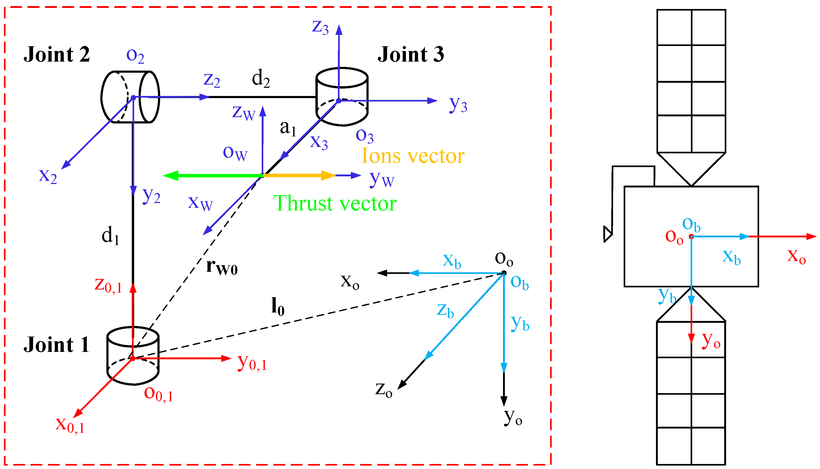
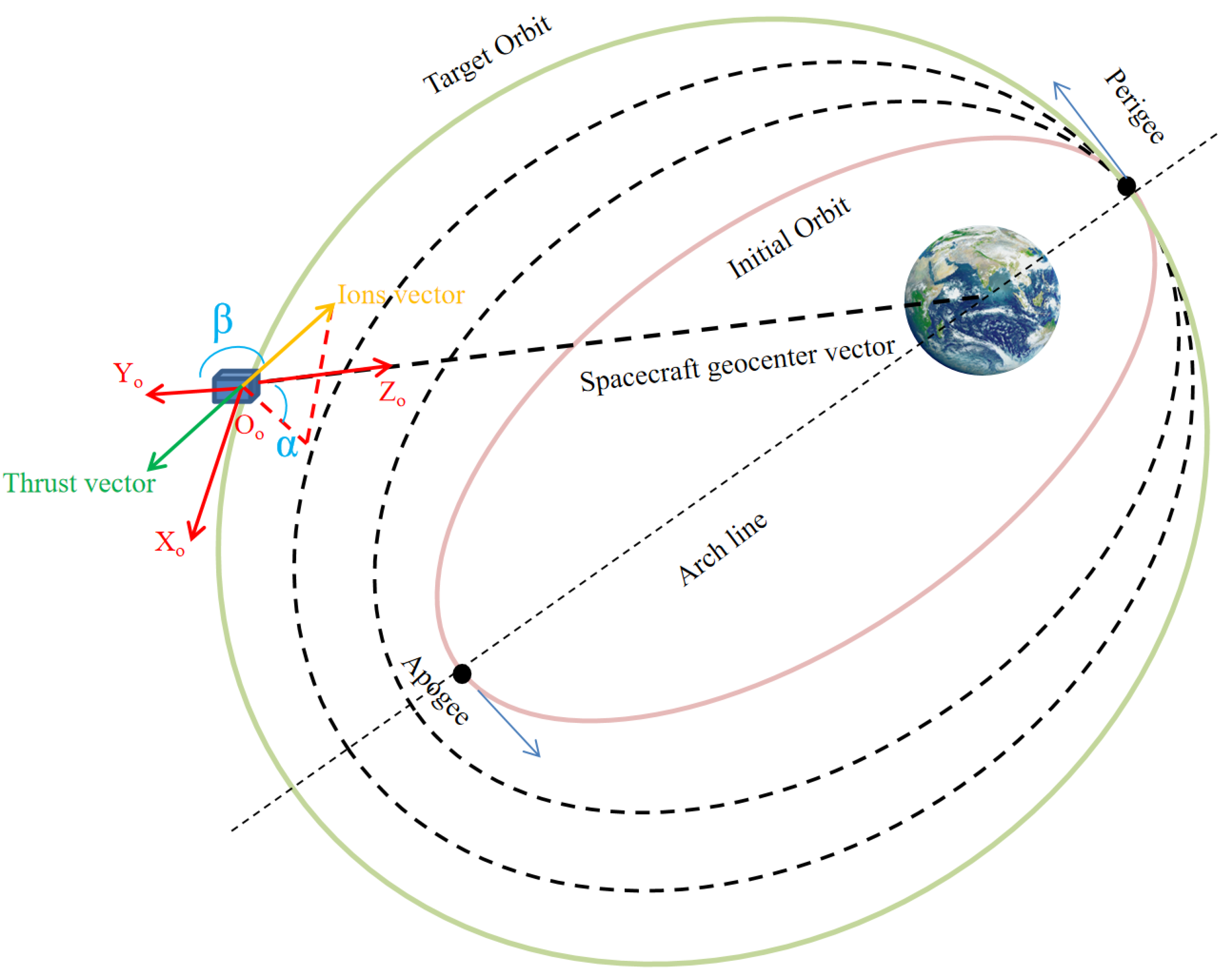
2.1. Modeling of GTO-GEO Transfer Satellite Based on Triple Orthogonal Configuration

2.1.1. Preparation

This paper proposes a triple orthogonal configuration of the gimbaled thruster boom to achieve the directional control of the thrust vector for the GTO-GEO orbit transfer process, as illustrated in Figure 1.

The coordinate system O_oX_oY_oZ_o is the spacecraft orbit coordinate system, and the spacecraft body coordinates system O_bX_bY_bZ_b origin coincides with the spacecraft orbit coordinate system O_oX_oY_oZ_o in this scheme. The coordinate system O₀X₀Y₀Z₀ is the base coordinate system of the gimbaled thruster boom, and the relative position vector between its origin and the origin of the spacecraft body coordinate system O_bX_bY_bZ_b is l₀. O_iX_iY_iZ_i (i = 1, 2, 3) represent the three linkages coordinate systems of the gimbaled thruster boom, respectively. The thruster is mounted along the X-axis direction of the spacecraft orbit coordinate system O_oX_oY_oZ_o. The joint lengths of joint 1 and joint 2 are d₁ and d₂, respectively, and the joint 3 linkage length is a₁. The position vector of the origin of the wrist coordinate system concerning the origin of the base coordinate system.

Remark 1.

To realize the re-orbit task, the projection of the required thrust vector direction in the spacecraft orbit coordinate system needs to be determined. If the angle is within the motion range, the joint can be controlled to adjust the thrust vector pointing. Otherwise, the needs to be adjusted the spacecraft attitude in conjunction with the gimbaled thruster boom. Also, it should be noted that in the proposed orthogonal configuration, the initial rotation angle of joint 2 is set to 90 deg.

The GTO-GEO orbit transfer process consists of two main phases: in-orbit plane adjustment and out-of-orbit plane adjustment. In the first phase, the spacecraft’s orbital plane should be adjusted to coincide with the GEO orbital plane. In the second phase, the spacecraft is accelerated along the orbital velocity direction at the apogee, which reduces the orbital eccentricity and increases the orbital semi-major axis until the orbit becomes circular. This circularization process helps align the current orbit with the GEO orbit.

The GTO-GEO orbital transfer thrust control method used in this paper is shown in Figure 2.

During the thruster start-up process, the thrust direction is divided into two directional components: the orbital and the out-of-orbit planes. The thrust control angle α is defined as the angle between the projection of the ions vector in the orbit plane and the direction of the spacecraft geocentric vector in the orbit coordinate system, with the ions vector pointing in the radial direction being positive. The thrust control angle β defined as the angle between the ions vector and the orbit plane, and the ions vector pointing to the direction of the spacecraft angular momentum is positive. To facilitate the study, the coupling between the inside and outside of the orbit plane is ignored in this paper, and the analytical solution of the thrust control angle is defined as follows:

$$\{\begin{array}{l}\mathsf{\alpha }=\arctan \left[-2\frac{\cot \frac{{\mathrm{J}}_{\mathrm{oribit}}}{2}}{\left({1+\mathrm{ecosJ}}_{\mathrm{oribit}}\right)}\left(1-{\mathrm{esin}}^2\frac{{\mathrm{J}}_{\mathrm{oribit}}}{2}\right)\right]\\ \mathsf{\beta }=-\frac{\mathsf{\pi }}{2}\sin \left(\mathrm{u}+\frac{\mathsf{\pi }}{2}\right)\end{array},$$

(1)

where e is the spacecraft orbit eccentricity, J_orbit is the spacecraft orbit true perigee angle, and u is the spacecraft orbit latitude amplitude angle.

For the scheme proposed in this paper, the mapping between the required thrust control angle of the spacecraft and the attitude angle of the spacecraft body coordinate system concerning the orbital coordinate system is given as follows:

$$\{\begin{array}{l}\mathsf{\alpha }=-{\mathsf{\Theta }}_{\mathrm{y}}\hfill \\ \mathsf{\beta }=-{\mathsf{\Theta }}_{\mathrm{z}}\hfill \end{array},$$

(2)

where Θ_y denotes the pitch angle of the spacecraft body and coordinates system with respect to the spacecraft orbit coordinate system, and Θ_z indicates the yaw angle of the spacecraft body coordinate system concerning the spacecraft orbit coordinate system.

2.1.2. GTO-GEO Transfer Spacecraft Kinematics and Dynamics

The GTO-GEO transfer spacecraft kinematics and dynamics are given as follows:

$${\dot{\mathit{r}}}_{\mathrm{i}}={\mathit{v}}_{\mathrm{i}},$$

(3)

$${\dot{\mathit{v}}}_{\mathrm{i}}=-\mathsf{\mu }\frac{{\mathit{r}}_{\mathrm{i}}}{{\Vert {\mathit{r}}_{\mathrm{i}}\Vert }^3}+{\mathit{a}}_{\mathrm{d}}+\frac{1}{{\mathrm{m}}_{\mathrm{b}}}{\mathit{C}}_{\mathrm{ib}}{\mathit{f}}_{\mathrm{thrust},\mathrm{b}},$$

(4)

$${\dot{\mathit{q}}}_{\mathrm{bo},\mathrm{b}}=\frac{1}{2}\left({\mathit{q}}_{\mathrm{bo},\mathrm{b}}^{\times }{\mathit{\omega }}_{\mathrm{bo},\mathrm{b}}+q_{\mathrm{bo},\mathrm{b}1}{\mathit{I}}_{3\times 3}{\mathit{\omega }}_{\mathrm{bo},\mathrm{b}}\right),$$

(5)

$$\begin{array}{l}{\dot{\mathit{\omega }}}_{\mathrm{bo},\mathrm{b}}={\mathit{J}}_{\mathrm{body}}^{-1}\left\{-{\left({\mathit{C}}_{\mathrm{bo}}{\mathit{\omega }}_{\mathrm{oi},\mathrm{o}}+{\mathit{\omega }}_{\mathrm{bo},\mathrm{b}}\right)}^{\times }\left[{\mathit{J}}_{\mathrm{body}}\left({\mathit{C}}_{\mathrm{bo}}{\mathit{\omega }}_{\mathrm{oi},\mathrm{o}}+{\mathit{\omega }}_{\mathrm{bo},\mathrm{b}}\right)+{\mathit{h}}_{\mathrm{f}}+{\mathit{\tau }}_{\mathrm{d}}+{\mathit{\tau }}_{\mathrm{c}}+{\mathit{\tau }}_{\mathrm{thrust},\mathrm{b}}\right]\right\}\\ \begin{array}{ccc}& & \end{array}+{\mathit{\omega }}_{\mathrm{bo},\mathrm{b}}^{\times }{\mathit{C}}_{\mathrm{bo}}{\mathit{\omega }}_{\mathrm{oi},\mathrm{o}}\end{array}$$

(6)

where ${\mathit{r}}_{\mathrm{i}}$ is the position vector of the spacecraft with respect to the center of the Earth in the ECI, ${\mathit{v}}_{\mathrm{i}}$ is the velocity vector of the spacecraft with respect to the center of the Earth in the geocentric inertial coordinate system, μ is the earth’s gravitational parameter, ${\mathit{a}}_{\mathrm{d}}$ is the perturbation acceleration of the spacecraft, ${\mathrm{m}}_{\mathrm{b}}$ is the mass of the spacecraft, ${\mathit{C}}_{\mathrm{ib}}$ is the conversion matrix of the spacecraft body coordinate system to the ECI, ${\mathit{f}}_{\mathrm{thrust},\mathrm{b}}$ is the projection of the thrust vector of the thrusters in the spacecraft body coordinate system, ${\mathit{q}}_{\mathrm{bo},\mathrm{b}}$ is the projection of the vector part of the attitude quaternion of the spacecraft body coordinate system with respect to the spacecraft orbit coordinate system under the spacecraft body coordinate system, ${\mathit{q}}_{\mathrm{bo},\mathrm{b}1}$ is the scalar part of the attitude quaternion of the spacecraft body coordinate system with respect to the spacecraft orbit coordinate system, ${\mathit{\omega }}_{\mathrm{bo},\mathrm{b}}$ is the projection of the angular velocity vector of the spacecraft body coordinate system with respect to the spacecraft orbit coordinate system under the spacecraft body coordinate system, ${\mathit{J}}_{\mathrm{body}}$ is the spacecraft inertia matrix, ${\mathit{C}}_{\mathrm{bo}}$ is the conversion matrix from the spacecraft orbit coordinate system to the spacecraft body coordinate system matrix, ${\mathit{\omega }}_{\mathrm{oi},\mathrm{o}}$ is the projection of the angular velocity vector of the spacecraft orbit coordinate system with respect to the geocentric inertial coordinate system under the spacecraft orbital coordinate system, ${\mathit{h}}_{\mathrm{f}}$ is the angular momentum of the spacecraft mounted flywheel, ${\mathit{\tau }}_{\mathrm{d}}$ is the disturbance moment of the spacecraft which takes into account the non-spherical uptake of the Earth, atmospheric drag and solar pressure, ${\mathit{\tau }}_{\mathrm{c}}$ is the control moment of the spacecraft, and ${\mathit{\tau }}_{\mathrm{thrust},\mathrm{b}}$ is the projection of the coupling moment generated by the thruster to the spacecraft attitude control process under the spacecraft body coordinate system.

The direction of the thrust vector is controlled by three rotational joints. And $\mathit{\theta }={\left[\begin{array}{ccc}{\mathsf{\theta }}_1& {\mathsf{\theta }}_2& {\mathsf{\theta }}_3\end{array}\right]}^{\mathrm{T}}$ denotes the angle of rotation of each joint. In the spacecraft body coordinate system, the thrust vector, as well as the coupling moment, can be written as:

$${\mathit{f}}_{\mathrm{thrust},\mathrm{b}}={\mathit{C}}_{\mathrm{Wb}}^{\mathrm{T}}\left[\begin{array}{c}f\\ 0\\ 0\end{array}\right]={\left({\mathit{C}}_{\mathrm{W}0}{\mathit{C}}_{\mathrm{bz}}\left(\frac{\mathsf{\pi }}{2}\right){\mathit{C}}_{\mathrm{bx}}\left(\frac{\mathsf{\pi }}{2}\right)\right)}^{\mathrm{T}}\left[\begin{array}{c}f\\ 0\\ 0\end{array}\right],$$

(7)

$${\mathit{\tau }}_{\mathrm{thrust},\mathrm{b}}={\left({\mathit{r}}_{\mathrm{W}0}+{\mathit{l}}_0\right)}^{\times }{\mathit{f}}_{\mathrm{thrust},\mathrm{b}}$$

(8)

where f is the thrust magnitude, ${\mathit{C}}_{\mathrm{Wb}}^{}$ is the transformation matrix from the spacecraft body coordinate system to the gimbaled thruster boom wrist coordinate system, ${\mathit{C}}_{\mathrm{bz}}$ and ${\mathit{C}}_{\mathrm{bx}}$ represent the attitude transformation matrix for an angle rotation about the j-axis (j = x, z), respectively. ${\mathit{C}}_{\mathrm{W}0}$ and ${\mathit{r}}_{\mathrm{W}0}$ represent the transformation matrix and the relative position vector from the base coordinate system to the wrist coordinate system of the gimbaled thruster boom.

The combined transformation matrix ${\mathit{T}}_{0\mathrm{W}}$ can be written as follows:

$${\mathit{T}}_{0\mathrm{W}}=\left[\begin{array}{cccc}{\mathrm{c}}_1{\mathrm{c}}_2{\mathrm{c}}_3{-\mathrm{s}}_1{\mathrm{s}}_3& {-\mathrm{s}}_1{\mathrm{c}}_3{-\mathrm{c}}_1{\mathrm{c}}_2{\mathrm{s}}_3& {\mathrm{c}}_1{\mathrm{s}}_2& {\mathrm{a}}_1\left({\mathrm{s}}_1{\mathrm{s}}_3{-\mathrm{c}}_1{\mathrm{c}}_2{\mathrm{c}}_3\right){+\mathrm{d}}_2{\mathrm{c}}_1{\mathrm{s}}_2{-\mathrm{d}}_1{\mathrm{s}}_1\\ {\mathrm{c}}_1{\mathrm{s}}_3{+\mathrm{c}}_2{\mathrm{c}}_3{\mathrm{s}}_1& {\mathrm{c}}_1{\mathrm{c}}_3{-\mathrm{s}}_1{\mathrm{c}}_2{\mathrm{s}}_3& {\mathrm{s}}_1{\mathrm{s}}_2& {\mathrm{a}}_1\left({\mathrm{c}}_1{\mathrm{s}}_3{+\mathrm{c}}_2{\mathrm{c}}_3{\mathrm{s}}_1\right){+\mathrm{d}}_1{\mathrm{c}}_1{+\mathrm{d}}_2{\mathrm{s}}_1{\mathrm{s}}_2\\ {-\mathrm{s}}_2{\mathrm{c}}_3& {\mathrm{s}}_2{\mathrm{s}}_3& {\mathrm{c}}_2& {\mathrm{d}}_2{\mathrm{c}}_2{-\mathrm{a}}_1{\mathrm{c}}_3{\mathrm{s}}_2\\ 0& 0& 0& 1\end{array}\right]$$

(9)

where ${\mathrm{s}}_{\mathrm{i}}$ (i = 1, 2, 3) and ${\mathrm{c}}_{\mathrm{i}}$ (i = 1, 2, 3) represent sin (θ_i) and cos (θ_i), respectively.

2.2. Gimbaled Thruster Boom Dynamics

2.2.1. Kinematics of the Thrust Vector-Regulated Gimbaled Thruster Boom

The coordinate system L_i is established at the center of mass of each connecting rod and the direction of the axes is taken to be the same as the direction of the main axis of inertia of the connecting rod to obtain the coordinate system L_i concerning the base coordinate system of the gimbaled thruster boom.

$${\mathit{g}}_{{0\mathrm{L}}_1}=\left[\begin{array}{cc}\begin{array}{c}\\ {\mathrm{I}}_3\\ \\ 0\end{array}& \begin{array}{c}0\\ 0\\ {\mathrm{r}}_1\\ 1\end{array}\end{array}\right], {\mathit{g}}_{{0\mathrm{L}}_2}=\left[\begin{array}{cc}\begin{array}{c}\\ {\mathrm{I}}_3\\ \\ 0\end{array}& \begin{array}{c}0\\ {\mathrm{r}}_2\\ {\mathrm{d}}_1\\ 1\end{array}\end{array}\right], {\mathit{g}}_{{0\mathrm{L}}_3}=\left[\begin{array}{cc}\begin{array}{c}\\ {\mathrm{I}}_3\\ \\ 0\end{array}& \begin{array}{c}{\mathrm{r}}_3\\ {\mathrm{d}}_2\\ {\mathrm{d}}_1\\ 1\end{array}\end{array}\right]$$

(10)

where ${\mathit{g}}_{0{\mathrm{L}}_1}$ (i = 1, 2, 3) represents the transformation matrix of the joint relative to the base, I₃ denotes 3 × 3 identity matrix.

In such a coordinate system, the linkage inertia matrix Ψ_i has the following general form.

$${\mathit{\Psi }}_{\mathrm{i}}=\left[\begin{array}{cccc}{\mathrm{m}}_{\mathrm{i}}& 0& 0& \begin{array}{cc}& \begin{array}{cc}& \end{array}\end{array}\\ 0& {\mathrm{m}}_{\mathrm{i}}& 0& \begin{array}{cc}& \begin{array}{cc}0& \end{array}\end{array}\\ 0& 0& {\mathrm{m}}_{\mathrm{i}}& \begin{array}{cc}& \begin{array}{cc}& \end{array}\end{array}\\ \begin{array}{c}\\ \begin{array}{c}\\ \end{array}\end{array}& \begin{array}{c}\\ \begin{array}{c}0\\ \end{array}\end{array}& \begin{array}{c}\\ \begin{array}{c}\\ \end{array}\end{array}& \begin{array}{ccc}\begin{array}{c}{\mathrm{I}}_{\mathrm{xi}}\\ 0\\ 0\end{array}& \begin{array}{c}0\\ {\mathrm{I}}_{\mathrm{yi}}\\ 0\end{array}& \begin{array}{c}0\\ 0\\ {\mathrm{I}}_{\mathrm{zi}}\end{array}\end{array}\end{array}\right],$$

(11)

where m_i is the mass of the linkage, I_xi, I_yi and I_zi are the moments of inertia of the i linkage, respectively. From this, the bit shape of the base coordinate system and the wrist coordinate system is obtained as follows:

$${\mathit{g}}_{0\mathrm{W}}=\left[\begin{array}{cc}\begin{array}{c}\\ {\mathrm{I}}_3\\ \\ 0\end{array}& \begin{array}{c}\left[\begin{array}{c}{\mathrm{a}}_1\\ {\mathrm{d}}_2\\ {\mathrm{d}}_1\end{array}\right]\\ 1\end{array}\end{array}\right],$$

(12)

To construct the kinematic rotation of the rotating joints, note that the unit vector of each joint axis of rotation ω_i (i = 1, 2, 3) is:

$${\mathit{\omega }}_1=\left[\begin{array}{c}0\\ 0\\ 1\end{array}\right], {\mathit{\omega }}_2=\left[\begin{array}{c}0\\ 1\\ 0\end{array}\right], {\mathit{\omega }}_3=\left[\begin{array}{c}0\\ 0\\ 1\end{array}\right],$$

(13)

Taking the points q_i (i = 1, 2, 3) on the axes respectively, thus:

$${\mathit{q}}_1=\left[\begin{array}{c}0\\ 0\\ 0\end{array}\right], {\mathit{q}}_2=\left[\begin{array}{c}0\\ 0\\ {\mathrm{d}}_1\end{array}\right], {\mathit{q}}_3=\left[\begin{array}{c}0\\ {\mathrm{d}}_2\\ {\mathrm{d}}_1\end{array}\right],$$

(14)

The motion spiral of each joint ξ_i (i = 1, 2, 3) is generated by:

$${\mathit{\xi }}_1=\left[\begin{array}{c}0\\ \begin{array}{c}0\\ \begin{array}{c}0\\ \begin{array}{c}0\\ \begin{array}{c}0\\ 1\end{array}\end{array}\end{array}\end{array}\end{array}\right], {\mathit{\xi }}_2=\left[\begin{array}{c}-{\mathrm{d}}_1\\ \begin{array}{c}0\\ \begin{array}{c}0\\ \begin{array}{c}0\\ \begin{array}{c}1\\ 0\end{array}\end{array}\end{array}\end{array}\end{array}\right], {\mathit{\xi }}_3=\left[\begin{array}{c}{\mathrm{d}}_2\\ \begin{array}{c}0\\ \begin{array}{c}0\\ \begin{array}{c}0\\ \begin{array}{c}0\\ 1\end{array}\end{array}\end{array}\end{array}\end{array}\right] ,$$

(15)

Then, the kinematic positive solution mapping of the gimbaled thruster boom has the following form.

$$\{\begin{array}{l}{\mathit{g}}_{0\mathrm{W}}(\mathit{\theta })={\mathit{e}}^{{\mathit{\xi }}_1{\theta }_1}{\mathit{e}}^{{\mathit{\xi }}_2{\theta }_2}{\mathit{e}}^{{\mathit{\xi }}_3{\theta }_3}{\mathit{g}}_{0\mathrm{W}}\left(0\right)\hfill \\ {\mathit{e}}^{\mathit{\xi }\theta }=\left[\begin{array}{cc}{\mathit{e}}^{\mathit{\omega }\theta }& (\mathit{I}-{\mathit{e}}^{\mathit{\omega }\theta })({\mathit{\omega }}^{\times }\mathit{v})+\mathit{\omega }{\mathit{\omega }}^{\mathrm{T}}\mathit{v}\theta \\ 0_{3\times 1}& 1\end{array}\right]\hfill \\ {\mathit{e}}^{\mathit{\omega }\theta }=\mathit{I}+{\mathit{\omega }}^{\times }\sin \theta +{\mathit{\omega }}^{\times }{}^2(1-\cos \theta )\hfill \end{array},$$

(16)

where ${\mathit{e}}^{\omega \theta }\in S{O}_3\in {ℝ}^{3\times 3}$ and $\mathit{\theta }={\left[\begin{array}{ccc}{\mathsf{\theta }}_1& {\mathsf{\theta }}_2& {\mathsf{\theta }}_3\end{array}\right]}^{\mathrm{T}}$ denotes the angle of rotation of each joint. The exponential product formula expands the equations to obtain the kinematic positive solution mapping ${\mathit{g}}_{0\mathrm{W}}\left(\mathit{\theta }\right)$ of the thrust vector regulating the gimbaled thruster boom.

2.2.2. Thrust Vector Adjustment Dynamics

To calculate the inertia matrix of the gimbaled thruster boom, it is easy to see that:

$$\{\begin{array}{l}{\mathit{V}}_{{0\mathrm{L}}_1}^{\mathrm{b}}={\mathit{\xi }}_1^{+}{\dot{\mathit{\theta }}}_1={\mathit{J}}_1\left(\mathit{\theta }\right)\dot{\mathit{\theta }}\hfill \\ {\mathit{V}}_{{0\mathrm{L}}_2}^{\mathrm{b}}={\mathit{\xi }}_1^{+}{\dot{\mathit{\theta }}}_1+{\mathit{\xi }}_2^{+}{\dot{\mathit{\theta }}}_2={\mathit{J}}_2(\mathit{\theta })\dot{\mathit{\theta }}\hfill \\ {\mathit{V}}_{{0\mathrm{L}}_3}^{\mathrm{b}}={\mathit{\xi }}_1^{+}{\dot{\mathit{\theta }}}_1+{\mathit{\xi }}_2^{+}{\dot{\mathit{\theta }}}_2+{\mathit{\xi }}_3^{+}{\dot{\mathit{\theta }}}_3={\mathit{J}}_3\left(\mathit{\theta }\right)\dot{\mathit{\theta }}\hfill \end{array} ,$$

(17)

where ${\mathit{V}}_{{0\mathrm{L}}_{\mathrm{i}}}^{\mathrm{b}}$ (i = 1, 2, 3) represents the projection of the velocity of the joint concerning the base, ${\mathit{\xi }}_{\mathrm{i}}^{+}$ (i = 1, 2, 3) is used to calculate the Jacobi matrix J_i (i = 1, 2, 3) for each connecting rod.

Thus:

$${\mathit{J}}_1=\left[\begin{array}{ccc}0& 0& 0\\ 0& 0& 0\\ 0& 0& 0\\ 0& 0& 0\\ 0& 0& 0\\ 1& 0& 0\end{array}\right], {\mathit{J}}_2=\left[\begin{array}{ccc}-{\mathrm{r}}_2{\mathrm{c}}_2& 0& 0\\ 0& 0& 0\\ -{\mathrm{r}}_2{\mathrm{s}}_2& 0& 0\\ -{\mathrm{s}}_2& 0& 0\\ 0& 1& 0\\ {\mathrm{c}}_2& 0& 0\end{array}\right], {\mathit{J}}_3=\left[\begin{array}{ccc}-{\mathrm{d}}_2{\mathrm{c}}_2& 0& 0\\ {\mathrm{c}}_2{(\mathrm{r}}_3{+\mathrm{d}}_2{\mathrm{s}}_3)& 0& {\mathrm{r}}_3\\ -{\mathrm{s}}_3{(\mathrm{d}}_2{+\mathrm{r}}_3{\mathrm{s}}_3)& -{\mathrm{r}}_3{\mathrm{c}}_3& 0\\ -{\mathrm{c}}_3{\mathrm{s}}_2& {\mathrm{s}}_3& 0\\ {\mathrm{s}}_2{\mathrm{s}}_3& {\mathrm{c}}_3& 0\\ {\mathrm{c}}_2& 0& 1\end{array}\right],$$

(18)

The inertia matrix of the system is $\mathit{M}(\mathit{\theta })={\displaystyle \sum _{\mathrm{i}=1}^3{\mathit{J}}_{\mathrm{i}}^{\mathrm{T}}{\mathit{\psi }}_{\mathrm{i}}{\mathit{J}}_{\mathrm{i}}}$, and the Gauche and centrifugal forces can be obtained from the inertia matrix by the following equation.

$${\mathit{C}}_{\mathrm{ij}}(\mathit{\theta },\dot{\mathit{\theta }})={\displaystyle \sum _{\mathrm{k}=1}^3{\mathit{\Gamma }}_{\mathrm{ijk}}{\dot{\mathit{\theta }}}_{\mathrm{k}}}=\frac{1}{2}{\displaystyle \sum _{\mathrm{k}=1}^3\left\{\frac{\partial {\mathit{M}}_{\mathrm{ij}}}{\partial {\mathit{\theta }}_{\mathrm{k}}}+\frac{\partial {\mathit{M}}_{\mathrm{ik}}}{\partial {\mathit{\theta }}_{\mathrm{j}}}-\frac{\partial {\mathit{M}}_{\mathrm{kj}}}{\partial {\mathit{\theta }}_{\mathrm{i}}}\right\}}{\dot{\mathit{\theta }}}_{\mathrm{k}},$$

(19)

Finally, the forces acting on the gimbaled thruster boom can be expressed as:

$$\mathit{N}(\mathit{\theta },\dot{\mathit{\theta }})=\frac{\partial \mathit{V}}{\partial \mathit{\theta }},$$

(20)

where V represents the potential energy, which can be expressed as:

$$\mathit{V}(\mathit{\theta }{)=\mathrm{m}}_1{\mathrm{gh}}_1\left(\mathit{\theta }{)+\mathrm{m}}_2{\mathrm{gh}}_2\right(\mathit{\theta }{)+\mathrm{m}}_3{\mathrm{gh}}_3\left(\mathit{\theta }\right),$$

(21)

where h_i is the height of the center of mass of the ith rod.

The transformation matrix of each linkage centre-of-mass coordinate system with respect to the base coordinate system can be obtained using the positive kinematic positive solution mapping formula.

$$\{\begin{array}{l}{\mathit{g}}_{{0\mathrm{L}}_1}(\mathit{\theta })={\mathit{e}}^{{\mathit{\xi }}_1{\mathit{\theta }}_1}{\mathit{g}}_{{0\mathrm{L}}_1}\left(0\right)\hfill \\ {\mathit{g}}_{{0\mathrm{L}}_2}(\mathit{\theta })={\mathit{e}}^{{\mathit{\xi }}_1{\mathit{\theta }}_1}{\mathit{e}}^{{\mathit{\xi }}_2{\mathit{\theta }}_2}{\mathit{g}}_{{0\mathrm{L}}_2}\left(0\right)\hfill \\ {\mathit{g}}_{{0\mathrm{L}}_3}(\mathit{\theta })={\mathit{e}}^{{\mathit{\xi }}_1{\mathit{\theta }}_1}{\mathit{e}}^{{\mathit{\xi }}_2{\mathit{\theta }}_2}{\mathit{e}}^{{\mathit{\xi }}_3{\mathit{\theta }}_3}{\mathit{g}}_{{0\mathrm{L}}_3}\left(0\right)\hfill \end{array},$$

(22)

Therefore, the height of the center of mass of each connecting rod can be obtained as follows:

$$\{\begin{array}{l}{\mathrm{h}}_1{=\mathrm{r}}_0\hfill \\ {\mathrm{h}}_2{=\mathrm{d}}_1\hfill \\ {\mathrm{h}}_3{=\mathrm{d}}_1-{\mathrm{r}}_2{\mathrm{c}}_3{\mathrm{s}}_2\hfill \end{array},$$

(23)

Taking it into the potential energy formula and differentiating it, yields:

$$\mathit{N}(\mathit{\theta },\dot{\mathit{\theta }})=\frac{\partial \mathit{V}}{\partial \mathit{\theta }}=\left[\begin{array}{c}0\\ -{\mathrm{gm}}_3{\mathrm{r}}_2{\mathrm{c}}_2{\mathrm{c}}_3\\ {\mathrm{gm}}_3{\mathrm{r}}_2{\mathrm{s}}_2{\mathrm{s}}_3\end{array}\right],$$

(24)

So far, the kinetic equation of the gimbaled thruster boom can be obtained as follows:

$${\mathit{\tau }}_{\mathrm{ARM}}={\left[\begin{array}{ccc}{\mathit{\tau }}_1& {\mathit{\tau }}_2& {\mathit{\tau }}_3\end{array}\right]}^{\mathrm{T}}=\mathit{M}\left(\mathit{\theta }\right)\ddot{\mathit{\theta }}+\mathit{C}(\mathit{\theta },\dot{\mathit{\theta }})+\mathit{N}(\mathit{\theta },\dot{\mathit{\theta }}),$$

(25)

where ${\mathit{\tau }}_{\mathrm{ARM}}$ is the driving moment of each rotating joint, $\mathit{M}\left(\mathit{\theta }\right)$ is the inertia matrix of the gimbaled thruster boom, $\mathit{C}(\mathit{\theta },\dot{\mathit{\theta }})$ is the Gauche and centrifugal forces on the system, and $\mathit{N}(\mathit{\theta },\dot{\mathit{\theta }})$ is the potential energy equation of the system.

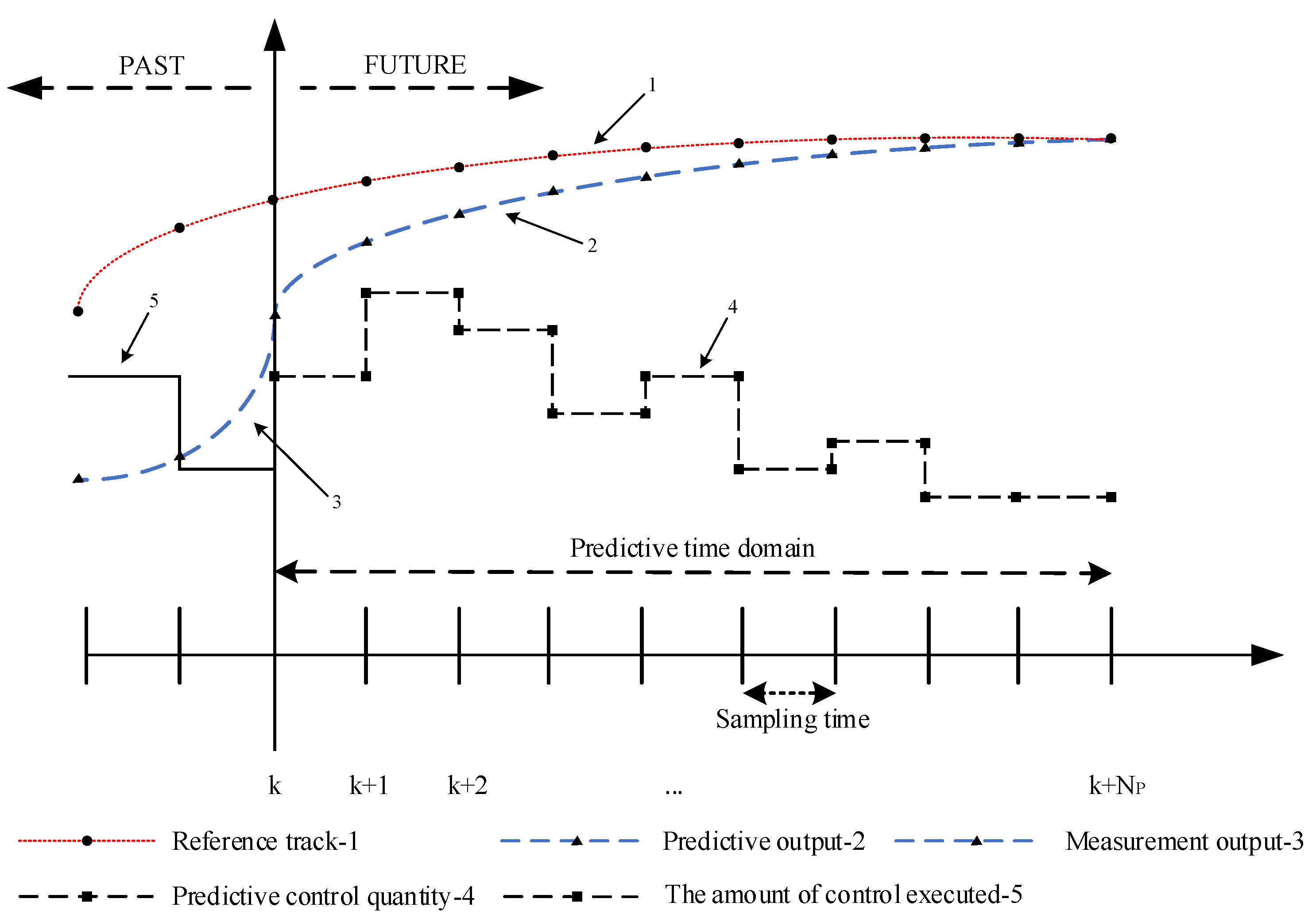
3. Planning Algorithm Design

3.1. Controller Description

In the above section, we have determined the relationship between the thrust angle and the joint angle of the gimbal thruster boom during the GTO-GEO transfer. The next step is to perform drive control for the gimbal thruster boom. Considering the thrust angle adjustment demand of fast response and high accuracy, MPC has been applied in various research fields with its convenient modeling and high robustness [24,25]. Therefore, this paper uses MPC to implement the drive control of the gimbaled thruster boom during GTO-GEO transfer.

Considering the gimbaled thruster boom dynamics as shown in Equation (25), writing $\ddot{\theta }$ to the left side of the equation yields:

$$\ddot{\mathit{\theta }}=\mathit{M}{(\mathit{\theta })}^{-1}(-\mathit{C}(\mathit{\theta },\dot{\mathit{\theta }})-\mathit{N}(\mathit{\theta },\dot{\mathit{\theta }}))+\mathit{M}{(\mathit{\theta })}^{-1}\mathit{\tau },$$

(26)

Defining the state of the system $\mathit{x}={\left[\mathit{\theta } \dot{\mathit{\theta }}\right]}^{\mathrm{T}}$, the nonlinear state space equation of the system can be expressed as follows:

$$\dot{\mathit{x}}=\mathit{f}(\mathit{x})+\mathit{g}(\mathit{x})\mathit{u},$$

(27)

where f(x) and g(x) can be obtained from equation Equation (26). Defining ${\mathit{x}}_0$ as a certain state, u denotes the control input, then the above equation can be linearized around ${\mathit{x}}_0$ by using Taylor’s Expanded Form as follows:

$$\dot{\mathit{x}}=\mathit{f}\left({\mathit{x}}_0\right)+{\mathit{f}}^{\prime }\left(\mathit{x}\right)|{}_{x=x_0}(\mathit{x}-{\mathit{x}}_0)+\mathit{g}({\mathit{x}}_0)\mathit{u},$$

(28)

Therefore, the linear state space equation can be expressed as follows.

$$\dot{\mathit{x}}=\mathit{A}\mathit{x}+\mathit{B}\mathit{u}+\mathit{C},$$

(29)

where $\mathit{A}={\mathit{f}}^{\prime }({\mathit{x}}_0),\mathit{B}=\mathit{g}({\mathit{x}}_0),\mathit{C}=\mathit{f}({\mathit{x}}_0)-{\mathit{f}}^{\prime }\left({\mathit{x}}_0\right){\mathit{x}}_0$.

Considering the different initialization points, the linear state space equation can be discretized as follows.

$${\mathit{x}}_{\mathrm{k}+1}={\mathit{A}}_{\mathrm{k}}{\mathit{x}}_{\mathrm{k}}+{\mathit{B}}_{\mathrm{k}}{\mathit{u}}_{\mathrm{k}}+{\mathit{C}}_{\mathrm{k}},$$

(30)

where ${\mathit{A}}_{\mathrm{k}}$, ${\mathit{B}}_{\mathrm{k}}$ and ${\mathit{C}}_{\mathrm{k}}$ represent the different linearization points, respectively.

Since the model predictive control is a rolling finite-time-domain optimization strategy, the planning allocation can be determined in each sampling unit. This kind of online iteration can be used to guarantee optimal allocation. Therefore, the model predictive control is adopted for planning the allocation of the gimbaled thruster boom in this paper.

Taking the linear state space equation expressed by iteration yields:

$$\begin{array}{ll}\left[\begin{array}{l}{\mathit{x}}_{\mathrm{k}+1}\\ {\mathit{x}}_{\mathrm{k}+2}\\ ⋮\\ {\mathit{x}}_{\mathrm{k}+\mathrm{N}}\end{array}\right]& =\left[\begin{array}{c}{\mathit{A}}_{\mathrm{k}}{\mathit{x}}_k\\ {\mathit{A}}_{\mathrm{k}+1}{\mathit{A}}_k{\mathit{x}}_k\\ ⋮\\ {\mathit{A}}_{\mathrm{k}+\mathrm{N}-1}\cdots {\mathit{A}}_{\mathrm{k}+1}{\mathit{A}}_k{\mathit{x}}_k\end{array}\right]+\left[\begin{array}{c}{\mathit{B}}_k{\mathit{u}}_k\\ {\mathit{A}}_{\mathrm{k}+1}{\mathit{B}}_k{\mathit{u}}_k+{\mathit{B}}_{\mathrm{k}+1}{\mathit{u}}_{\mathrm{k}+1}\\ ⋮\\ {\mathit{A}}_{\mathrm{k}+\mathrm{N}-1}\cdots {\mathit{A}}_{\mathrm{k}+2}{\mathit{A}}_{\mathrm{k}+1}{\mathit{B}}_k{\mathit{u}}_k+\cdots +{\mathit{B}}_{\mathrm{k}+\mathrm{N}-1}{\mathit{u}}_{\mathrm{k}+\mathrm{N}-1}\end{array}\right]\\ & +\left[\begin{array}{c}{\mathit{C}}_k\\ {\mathit{A}}_{k+1}{\mathit{C}}_k+{\mathit{C}}_{k+1}\\ ⋮\\ {\mathit{A}}_{\mathrm{k}+\mathrm{N}-1}\cdots {\mathit{A}}_{\mathrm{k}+2}{\mathit{A}}_{\mathrm{k}+1}{\mathit{C}}_k+{\mathit{A}}_{\mathrm{k}+\mathrm{N}-1}\cdots {\mathit{A}}_{\mathrm{k}+2}{\mathit{C}}_{\mathrm{k}+1}+\cdots +{\mathit{A}}_{\mathrm{k}+\mathrm{N}-1}{\mathit{C}}_{\mathrm{k}+\mathrm{N}-1}+{\mathit{C}}_{\mathrm{k}+\mathrm{N}}\end{array}\right]\end{array},$$

(31)

Marking $\mathit{X}={\left[\begin{array}{lllll}{\mathit{x}}_{\mathrm{k}+1}\hfill & {\mathit{x}}_{\mathrm{k}+2}\hfill & {\mathit{x}}_{\mathrm{k}+3}\hfill & \cdots \hfill & {\mathit{x}}_{\mathrm{k}+\mathrm{N}}\hfill \end{array}\right]}^{\mathrm{T}}$, thus:

$$\begin{array}{ll}\mathit{X}& =\left[\begin{array}{cccc}{\mathit{B}}_{\mathrm{k}}& 0& \cdots & 0\\ {\mathit{A}}_{\mathrm{k}+1}{\mathit{B}}_{\mathrm{k}}& {\mathit{B}}_{\mathrm{k}+\mathrm{N}-1}& \cdots & 0\\ ⋮& ⋮& \ddots & ⋮\\ {\mathit{A}}_{\mathrm{k}+\mathrm{N}-1}\cdots {\mathit{A}}_{\mathrm{k}+2}{\mathit{A}}_{\mathrm{k}+1}{\mathit{B}}_{\mathrm{k}}& {\mathit{A}}_{\mathrm{k}+\mathrm{N}-1}\cdots {\mathit{A}}_{\mathrm{k}+3}{\mathit{A}}_{\mathrm{k}+2}{\mathit{B}}_{\mathrm{k}+1}& \cdots & {\mathit{B}}_{\mathrm{k}+\mathrm{N}-1}\end{array}\right]\left[\begin{array}{c}{\mathit{u}}_{\mathrm{k}}\\ {\mathit{u}}_{\mathrm{k}+1}\\ ⋮\\ {\mathit{u}}_{\mathrm{k}+\mathrm{N}-1}\end{array}\right]\\ & +\left[\begin{array}{c}{\mathit{B}}_{\mathrm{k}}{\mathit{u}}_{\mathrm{k}}\\ {\mathit{A}}_{\mathrm{k}+1}{\mathit{B}}_{\mathrm{k}}{\mathit{u}}_{\mathrm{k}}+{\mathit{B}}_{\mathrm{k}+1}{\mathit{u}}_{\mathrm{k}+1}\\ ⋮\\ {\mathit{A}}_{\mathrm{k}+\mathrm{N}-1}\cdots {\mathit{A}}_{\mathrm{k}+2}{\mathit{A}}_{\mathrm{k}+1}{\mathit{B}}_{\mathrm{k}}{\mathit{u}}_{\mathrm{k}}+{\mathit{A}}_{\mathrm{k}+\mathrm{N}-1}\cdots {\mathit{A}}_{\mathrm{k}+3}{\mathit{A}}_{\mathrm{k}+2}{\mathit{B}}_{\mathrm{k}+1}{\mathit{u}}_{\mathrm{k}+1}+\cdots +{\mathit{B}}_{\mathrm{k}+\mathrm{N}-1}{\mathit{u}}_{\mathrm{k}+\mathrm{N}-1}\end{array}\right]\\ & +\left[\begin{array}{c}{\mathit{C}}_{\mathrm{k}}\\ {\mathit{A}}_{\mathrm{k}+1}{\mathit{C}}_{\mathrm{k}}+{\mathit{C}}_{\mathrm{k}+1}\\ ⋮\\ {\mathit{A}}_{\mathrm{k}+\mathrm{N}-1}\cdots {\mathit{A}}_{\mathrm{k}+2}{\mathit{A}}_{\mathrm{k}+1}{\mathit{C}}_{\mathrm{k}}+{\mathit{A}}_{\mathrm{k}+\mathrm{N}-1}\cdots {\mathit{A}}_{\mathrm{k}+2}{\mathit{C}}_{\mathrm{k}+1}+\cdots +{\mathit{A}}_{\mathrm{k}+\mathrm{N}-1}{\mathit{C}}_{\mathrm{k}+\mathrm{N}-1}+{\mathit{C}}_{\mathrm{k}+\mathrm{N}}\end{array}\right]\end{array},$$

(32)

Therefore, the planning allocation of the gimbaled thruster boom can be transformed into tracking optimization based on model predictive control as follows:

$$\{\begin{array}{l}\underset{\mathit{U}}{\min }\mathit{J}={\displaystyle \sum _{\mathrm{j}=\mathrm{k}}^{\mathrm{k}+\mathrm{N}-1}{\mathit{l}}_{\mathrm{e}}(\mathit{x}\left(\mathrm{j}\right),}\mathit{u}\left(\mathrm{j}\right))\\ \begin{array}{l}\mathrm{s}.\mathrm{t}.\mathit{x}(\mathrm{j}+1)=\mathit{h}(\mathit{x}\left(\mathrm{j}\right),\mathit{u}\left(\mathrm{j}\right))\hfill \\ \mathit{u}\left(\mathrm{t}\right)\in \mathbb{U}\hfill \\ \mathit{x}\left(\mathrm{t}\right)\in \mathbb{X}\hfill \\ \mathit{x}(\mathrm{k}+\mathrm{N})={\mathit{x}}_{\mathrm{s}}\hfill \end{array}\end{array},$$

(33)

where the function ${\mathit{l}}_{\mathrm{e}}(\mathit{x}\left(\mathrm{j}\right),\mathit{u}\left(\mathrm{j}\right))$ represents each tracking step’s objective, the set of linear time-varying systems Equation (30), and the sets $\mathbb{U}$ $\mathbb{X}$ denote the set of constraints on the inputs and states. Let the tracking problem have an equilibrium point, set as ${\mathit{x}}_{\mathrm{s}}$, and use ${\mathit{x}}_{\mathrm{s}}$ to describe the stability conveniently, which can be obtained from the following equation.

$$\{\begin{array}{l}({\mathit{x}}_s,{\mathit{u}}_s)=\mathrm{argmin}{\mathit{l}}_{\mathrm{e}}(\mathit{x},\mathit{u})\hfill \\ \mathrm{s}.\mathrm{t}.\mathit{x}=\mathit{h}(\mathit{x},\mathit{u})\hfill \\ (\mathit{x},\mathit{u})\in {\mathbb{X}}_{\mathrm{e}}\times \mathbb{U}\hfill \end{array},$$

(34)

where ${\mathbb{X}}_{\mathrm{e}}$ is the robust control invariant set [24], i.e., for any $\forall \mathit{x}\in {\mathbb{X}}_{\mathrm{e}}$, $\exists \mathit{u}\in \mathbb{U}$, such that $\mathit{h}(\mathit{x},\mathit{u})\in {\mathbb{X}}_{\mathrm{e}}$. The computation of the robust control invariant set can be referred to in the literature [25]. According to the description above, the planning allocation of the gimbaled thruster boom can be demonstrated in Figure 3. In Section 2, it has been determined how the thrust angle changes. Therefore, we need to adjust the thrust angle by gimbaled thruster boom in this section.

3.2. Stability Analysis

To demonstrate the stability of the planning allocation of the gimbaled thruster boom, the following assumptions are made.

Assumption 1.

The robust control invariant set ${\mathbb{X}}_{\mathrm{e}}$ has been obtained.

Assumption 2.

The nominal system $\mathit{x}(\mathrm{j}+1)=\mathit{h}(\mathit{x}\left(\mathrm{j}\right),\mathit{u}\left(\mathrm{j}\right))$ is strongly dissipative concerning the supply rate $\mathit{s}(\mathit{x},\mathit{u})$, i.e., there exists a continuous storage function $\mathit{\lambda }(\cdot )$ and a ${\mathit{K}}_{\infty }$ function $\mathit{\alpha }(\cdot )$ such that the following equation holds for any $\mathit{x}\in \mathbb{X}$ and $\mathit{u}\in \mathbb{U}$.

$$\mathit{\lambda }(\mathit{h}(\mathit{x},\mathit{u}))-\mathit{\lambda }\left(\mathit{x}\right)\le \mathit{s}(\mathit{x},\mathit{u})-\mathit{\alpha }\left(\Vert \mathit{x}-{\mathit{x}}_{\mathrm{s}}\Vert \right),$$

(35)

where $\mathit{s}(\mathit{x},\mathit{u})={\mathit{l}}_{\mathrm{e}}(\mathit{x},\mathit{u})-{\mathit{l}}_{\mathrm{e}}({\mathit{x}}_{\mathrm{s}},{\mathit{u}}_{\mathrm{s}})$ [26]. The ${\mathit{K}}_{\infty }$ function is defined as an unbounded continuous function $\mathsf{\alpha }:[0,\mathrm{a})\to [0,\infty )$ that is strictly increasing and satisfies $\mathsf{\alpha }\left(0\right)=0$.

Assumption 3.

Defining the set of N-steps reachable concerning the equilibrium point ${\mathit{x}}_{\mathrm{s}}$.

$${\mathbb{X}}_{\mathrm{N}}=\{\mathit{x}\left(0\right)\in \mathbb{X}|\exists \mathit{u}\left(\mathrm{k}\right)\in \mathbb{U},\mathrm{k}=0,\dots ,\mathrm{N}-1,\mathrm{satisfy} \mathit{x}\left(\mathrm{k}\right)\in \mathbb{X},\mathrm{k}=1,\dots ,\mathrm{N}\},$$

(36)

i.e., the set of all states that can reach ${\mathit{x}}_{\mathrm{s}}$ in N steps. Suppose ${\mathit{X}}_{\mathrm{N}}$ is a tight set and ${\mathit{x}}_{\mathrm{s}}\in \mathrm{int}({\mathbb{X}}_{\mathrm{N}})$, where $\mathrm{int}(\cdot )$ denotes the set interior.

Assumption 4.

There exists ${\mathit{K}}_{\infty }$ class of functions $\mathit{\gamma }(\cdot )$, such that for any $\mathit{x}\in {\mathbb{X}}_{\mathrm{N}}$, there exists a feasible solution to the optimization problem. Therefore, the following equation holds.

$${\displaystyle \sum _{\mathrm{i}=0}^{\mathrm{N}-1}\Vert \mathit{u}(\mathrm{k}+\mathrm{i})-{\mathit{u}}_{\mathrm{s}}\Vert \le \mathit{\gamma }(\Vert \mathit{x}-{\mathit{x}}_{\mathrm{s}}\Vert )},$$

(37)

Lemma 1 gives the stability of the nominal system concerning the equilibrium point ${\mathit{x}}_{\mathrm{s}}$ [27].

Lemma 1.

Consider the problem for the nominal system and assume that Assumption 1–4 holds, then there exists a function λ(·) for all, such that the condition Equation (35) holds. Defining the rolling cost function as follows:

$${\tilde{\mathit{l}}}_{\mathrm{e}}(\mathit{x},\mathit{u})={\mathit{l}}_{\mathrm{e}}(\mathit{x},\mathit{u})-{\mathit{l}}_{\mathrm{e}}({\mathit{x}}_{\mathrm{s}},{\mathit{u}}_{\mathrm{s}})+\mathit{\lambda }\left(\mathit{x}\right)-\mathit{\lambda }(\mathit{h}(\mathit{x},\mathit{u})),$$

(38)

Then the following control problem and optimization problem are equivalent.

$$\{\begin{array}{l}\underset{\mathit{U}}{\min }{\tilde{\mathit{V}}}_{\mathrm{N}}(\mathit{x}\left(\mathrm{k}\right),\mathit{u})={\displaystyle \sum _{\mathrm{j}=0}^{\mathrm{N}-1}{\tilde{\mathit{l}}}_{\mathrm{e}}}(\mathit{x}(\mathrm{k}+\mathrm{j}),\mathit{u}(\mathrm{k}+\mathrm{j}))\\ \begin{array}{l}\mathrm{s}.\mathrm{t}.\mathit{x}(\mathrm{j}+1)=\mathit{h}(\mathit{x}\left(\mathrm{j}\right),\mathit{u}\left(\mathrm{j}\right))\hfill \\ \mathit{u}\left(\mathrm{t}\right)\in \mathbb{U}\hfill \\ \mathit{x}\left(\mathrm{t}\right)\in \mathbb{X}\hfill \\ \mathit{x}(\mathrm{k}+\mathrm{N})={\mathit{x}}_{\mathrm{s}}\hfill \end{array}\end{array},$$

(39)

Furthermore, the optimal value of the problem, set to ${\tilde{\mathit{V}}}_{\mathrm{N}}^0(\cdot )$, is a Lyapunov function of the nominal closed-loop system with respect to the equilibrium point ${\mathit{x}}_{\mathrm{s}}$ after solving the control optimization problem.

Here, the actual system is the original nonlinear system, set as

$$\overline{\mathit{x}}(\mathrm{j}+1)=\overline{\mathit{h}}(\mathit{x}\left(\mathrm{j}\right),\mathit{u}\left(\mathrm{j}\right)),$$

(40)

We show that the optimal control rule obtained by solving the control optimization problem is also stable for the closed-loop system constituted by imposing it on the system when the deviation between the nominal and the actual system is bounded.

Assumption 5.

Let the deviation of the nominal system $\mathit{x}(\mathrm{k}+1)=\mathit{h}(\mathit{x}\left(\mathrm{k}\right),\mathit{u}\left(\mathrm{k}\right))$ and the actual system $\overline{\mathit{x}}(\mathrm{k}+1)=\overline{\mathit{h}}(\mathit{x}\left(\mathrm{k}\right),\mathit{u}\left(\mathrm{k}\right))$ be bounded, i.e.,

$$\Vert \mathit{x}(\mathrm{k}+1)-\overline{\mathit{x}}(\mathrm{k}+1)\Vert \le \mathrm{L},$$

(41)

Theorem 1.

Let Assumptions 1–5 hold and the partial derivative $\frac{\partial {\tilde{\mathit{V}}}_{\mathrm{N}}^0\left(\mathit{x}\right)}{\partial \mathit{x}}$ has an upper bound, i.e., for all $\mathit{x}\in \mathit{X}$, there is $\left|\frac{\partial {\tilde{V}}_{\mathrm{N}}^0\left(\mathit{x}\right)}{\partial \mathit{x}}\right|\le {\mathrm{K}}_{\mathrm{v}}$. Assume that there exists a real number ${\mathsf{\epsilon }}_{\mathrm{s}}>0$ and ${\mathsf{\rho }}_{\mathrm{s}}>0$, such that the following equation holds:

$$-{\mathsf{\alpha }(\mathsf{\rho }}_{\mathrm{s}}{)+\mathrm{K}}_{\mathrm{v}}{\mathrm{L}+\mathrm{HL}}^2\le -{\mathsf{\epsilon }}_{\mathrm{s}},$$

(42)

where $\mathsf{\alpha }(\cdot )$ is the function mentioned in Assumption 2 and H is a constant that expands with ${\tilde{\mathit{V}}}_{\mathrm{N}}^0\left(\mathit{x}\right)$ Taylor series. Let

$${\mathit{\Omega }}_{{\mathsf{\rho }}_{\min }}\subset {\mathbb{X}}_{\mathrm{e}}\subset {\mathit{\Omega }}_{{\mathsf{\rho }}_{\max }}\subset {\mathbb{X}}_{\mathrm{N}},$$

(43)

where ${\mathsf{\rho }}_{\min }$ is defined as:

$${\mathsf{\rho }}_{\min }=\max \{{\tilde{\mathit{V}}}_N^0{(\mathit{x}(\mathrm{k}+1\left)\right):\Vert \mathit{x}\left(\mathrm{k}\right)-{\mathit{x}}_{\mathrm{s}}\Vert }_2\le {\mathsf{\alpha }}^{-1}({\rho }_{\mathrm{s}}\left)\right\},$$

(44)

And ${\mathit{\Omega }}_{\mathsf{\rho }}$ is the level set of the Lyapunov function ${\tilde{\mathit{V}}}_{\mathrm{N}}^0(\cdot )$ mentioned in Lemma 1.

$${\mathit{\Omega }}_{\mathsf{\rho }}=\{\mathit{x}\in \mathbb{X}:{\tilde{\mathit{V}}}_{\mathrm{N}}^0\left(\mathit{x}\right)\le \mathsf{\rho }\},$$

(45)

The set ${\mathit{\Omega }}_{{\mathsf{\rho }}_{\max }}$ is the maximum level set within the set ${\mathbb{X}}_{\mathrm{N}}$. At this point for any initial value $\mathit{x}\left(0\right)\in {\mathit{\Omega }}_{{\mathsf{\rho }}_{\max }}$, the closed-loop system can converge to the robust control invariant set ${\mathbb{X}}_{\mathrm{e}}$ in a finite number of steps and remains within this set.

Proof of Theorem 1.

According to Assumption 5, thus a Taylor expansion of the Lyapunov function ${\tilde{\mathit{V}}}_{\mathrm{N}}^0\left(\mathit{x}\right)$ can be obtained as:

$${\tilde{\mathit{V}}}_{\mathrm{N}}^0\left(\right(\overline{\mathit{x}}(\mathrm{k}+1\left)\right)={\tilde{\mathit{V}}}_{\mathrm{N}}^0\left(\right(\mathit{x}(\mathrm{k}+1\left)\right)+\frac{\partial {\tilde{\mathit{V}}}_N^0\left(\mathit{x}\right)}{\partial \mathit{x}}|{}_{\mathit{x}(\mathrm{k}+1)}\cdot \left({\Vert \overline{x}(\mathrm{k}+1)-\mathit{x}(\mathrm{k}+1)\Vert }^2\right)\le \mathit{H}\left({\Vert \overline{x}(\mathrm{k}+1)-\mathit{x}(\mathrm{k}+1)\Vert }^2\right),$$

(46)

For $\mathit{x}\in {\mathbb{X}}_{\mathrm{e}}$, one can find a positive real number H, such that the higher order expansion term of the above equation satisfies that:

$$\mathit{H}\left({\Vert \overline{\mathit{x}}(\mathrm{k}+1)-\mathit{x}(\mathrm{k}+1)\Vert }^2\right)\le \mathit{H}{\Vert \overline{\mathit{x}}(\mathrm{k}+1)-\mathit{x}(\mathrm{k}+1)\Vert }^2,$$

(47)

Since the initial conditions are equal, we have the following:

$$\begin{array}{ll}{\tilde{\mathit{V}}}_{\mathrm{N}}^0(\overline{\mathit{x}}(\mathrm{k}+1\left)\right)& -{\tilde{\mathit{V}}}_{\mathrm{N}}^0(\overline{\mathit{x}}(k\left)\right)={\tilde{\mathit{V}}}_N^0(\overline{\mathit{x}}(\mathrm{k}+1\left)\right)-{\tilde{\mathit{V}}}_{\mathrm{N}}^0(\mathit{x}(\mathrm{k}\left)\right)\\ & \le {\tilde{\mathit{V}}}_{\mathrm{N}}^0(\mathit{x}(\mathrm{k}+1\left)\right)-{\tilde{\mathit{V}}}_N^0(\mathit{x}(\mathrm{k}\left)\right)+\frac{\partial {\tilde{\mathit{V}}}_{\mathrm{N}}^0(\mathit{x})}{\partial \mathit{x}}|{}_{\mathit{x}(\mathrm{k}+1)}\cdot (\overline{\mathit{x}}(\mathrm{k}+1)-\mathit{x}(\mathrm{k}+1\left)\right)\\ & +\mathit{H}\left({\Vert \overline{\mathit{x}}(\mathrm{k}+1)-\mathit{x}(\mathrm{k}+1)\Vert }^2\right)\le \mathit{\alpha }(\Vert \mathit{x}\left(\mathrm{k}\right)-{\mathit{x}}_{\mathrm{s}}\Vert )+{\mathit{K}}_{\mathrm{v}}\mathit{L}+\mathit{H}{\mathit{L}}^2\end{array}$$

(48)

If Equation (42) holds, there exists ${\mathsf{\rho }}_{\mathrm{s}}$, such that the last term of the above equation is less than ${-\mathsf{\epsilon }}_{\mathrm{s}}$. Since ${\mathsf{\rho }}_{\max }\ge {\mathsf{\rho }}_{\mathrm{s}}$, for all $\mathit{x}\left(\mathrm{k}\right)\in {\mathit{\Omega }}_{{\mathsf{\rho }}_{\max }}$, we have:

$${\tilde{\mathit{V}}}_{\mathrm{N}}^0(\overline{\mathit{x}}(\mathrm{k}+1\left)\right)-{\tilde{\mathit{V}}}_{\mathrm{N}}^0(\overline{\mathit{x}}(\mathrm{k}\left)\right)\le -{\mathsf{\epsilon }}_{\mathrm{s}},$$

(49)

The above equation illustrates that when $\Vert \mathit{x}\left(\mathrm{k}\right)-{\mathit{x}}_{\mathrm{s}}\Vert \ge {\mathsf{\rho }}_{\mathrm{s}}$, the Lyapunov function ${\tilde{\mathit{V}}}_{\mathrm{N}}^0\left(\overline{\mathit{x}}\left(\mathrm{k}\right)\right)$ continues to fall and eventually, the system state $\overline{\mathit{x}}\left(\mathrm{k}\right)$ will arrive within the set $\Vert \overline{\mathit{x}}-{\mathit{x}}_{\mathrm{s}}\Vert \le {\mathsf{\rho }}_{\mathrm{s}}$ in a finite number of steps. □

Given the definition of the set ${\mathit{\Omega }}_{{\mathsf{\rho }}_{\min }}$, the system will always be inside the set ${\mathit{\Omega }}_{{\mathsf{\rho }}_{\min }}$ when the system satisfies $\overline{\mathit{x}}\in {\mathit{\Omega }}_{{\mathsf{\rho }}_{\min }}$. Therefore, the actual closed-loop system will reach the set ${\mathbb{X}}_e$ in a finite number of steps and stay within ${\mathbb{X}}_e$ all the time, and the bounded stability is proved.

4. Planning Algorithm Design

4.1. Simulation Condition Configuration

To demonstrate the feasibility of the proposed GTO-GEO orbit transfer scheme based on the gimbaled thruster boom, this section will compare the orbit transfer scheme with the traditional quadrilateral layout in fixed direction. The parameters of the orbit and the gimbaled thruster boom involved in the simulation are shown in

Table 1. Simulation parameters.

Parameter		Value
Initial orbit	Perigee height	964 km
	Apogee height	35,741 km
	Orbital inclination	20.8 deg
Gimbaled thruster boom	Movement range of Joint 1	−90~0 deg
	Movement range of Joint 2	+75~+105 deg
	Movement range of Joint 3	−15~+15 deg

.

4.2. Result and Discussion

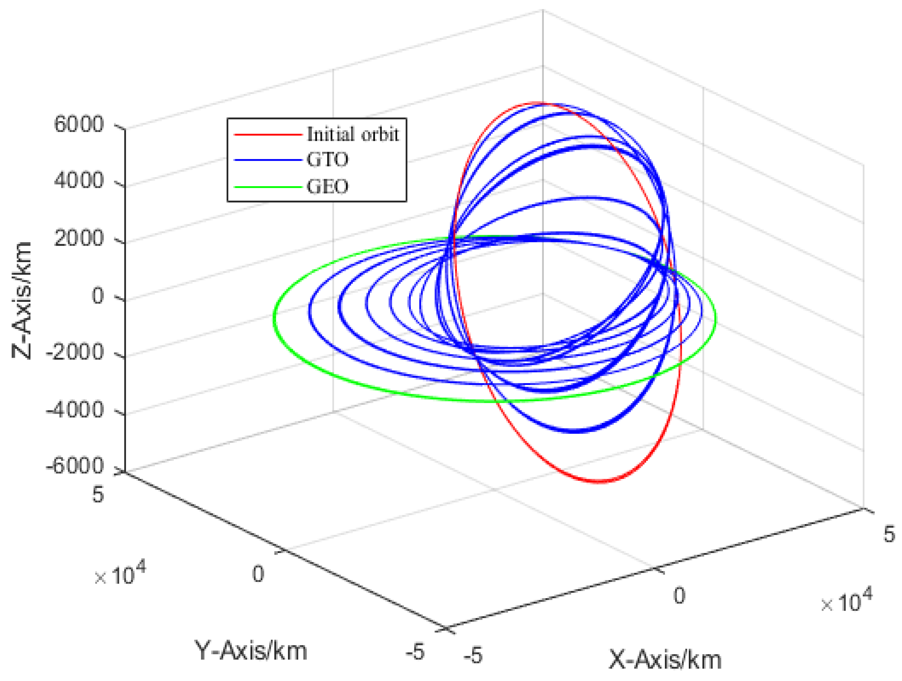
4.2.1. GTO-GEO Orbital Transfer Simulation Result and Discussion

The numerical simulation result of the GTO-GEO orbital transfer process are shown in Figure 4 and Figure 5.

As can be seen from Equation (1), the values of thrust control angle α and thrust control angle β are related to the satellite’s true proximity angle, and the thrust control angle in a single cycle is given in this paper considering that the trend of their changes is the same in each orbital cycle (Figure 6).

Remark 2.

From Equation (2), it can be seen that the thrust control angle α angle and β angle correspond to the negative values of pitch angle and yaw angle, respectively. Considering the motion angle of the Triple orthogonal Gimbaled Thruster Boom used in this paper, the thrust control angle requirement of${\Theta }_y\in [-90\mathrm{deg},0\mathrm{deg}),{\Theta }_z\in [-15\mathrm{deg},+15\mathrm{deg})$, the thrust control angle can be changed by driving joint 1 and joint 3, respectively, during the orbiting mission and then combined with the satellite attitude adjustment to complete the final thrust pointing requirement. The triple orthogonal gimbaled thruster boom can compensate for the required thrust vector pointing and save fuel consumption. At the same time, it can also significantly improve the efficiency of thrust vector adjustment due to its fast response time.

The change process of thrust control angle has been given in the GTO-GEO transfer process above, and we can make the thrust control angle meet the mission requirements by adjusting the spacecraft attitude and driving the gimbaled thruster boom joint motion. Figure 7, Figure 8, Figure 9 and Figure 10 give the simulation results of the pitch angle and yaw angle change process.

From the simulation result, it can be seen the thrusters are fixed to the spacecraft platform in the conventional scheme, so the full range of thrust control angle adjustment needs to be done through the attitude adjustment of the spacecraft. The proposed scheme can complete the above process by combining attitude adjustment and gimbaled thruster boom joint rotation. It saves the fuel required for the adjustment process and improves the efficiency of thrust vector adjustment, which has a high engineering application value.

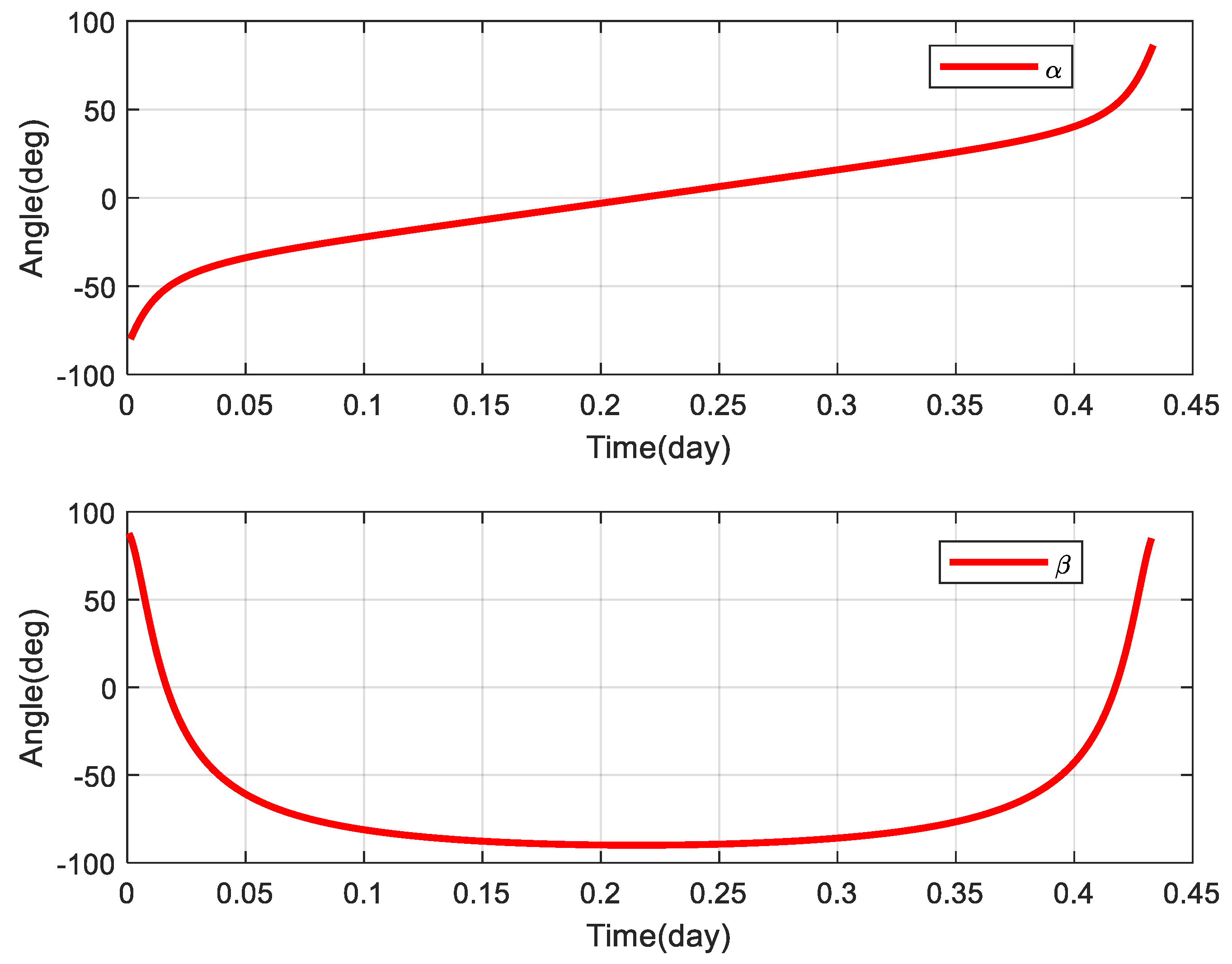
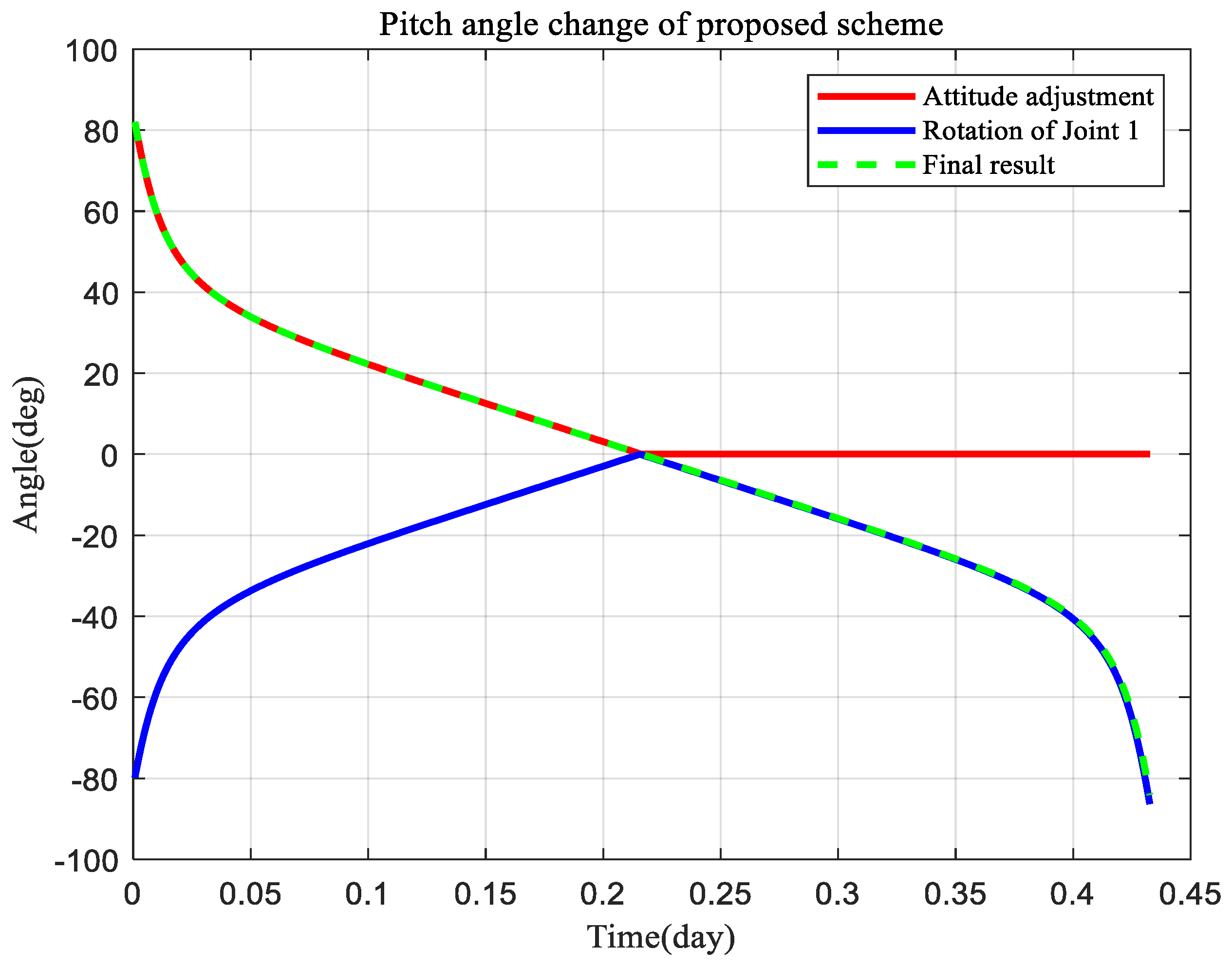
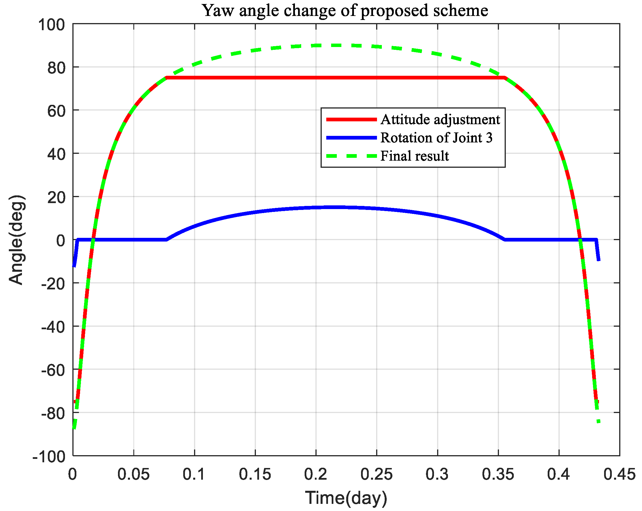
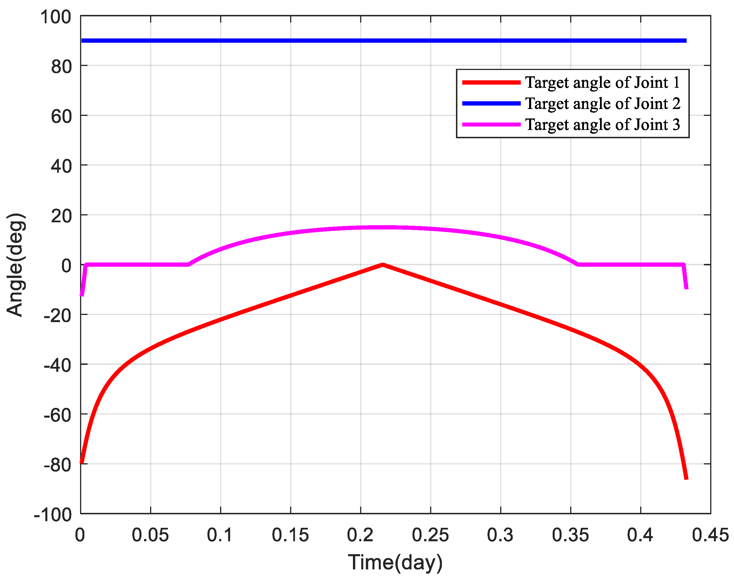
4.2.2. Gimbaled Thruster Boom Simulation Result and Discussion

In the previous section, we have determined the variation requirement of the thrust control angle by the GTO-GEO orbit transfer process, and based on this, we have obtained the target angles of each joint of the gimbaled thruster boom in this process, which denote $\mathit{\theta }={\left[\begin{array}{ccc}{\mathsf{\theta }}_1& {\mathsf{\theta }}_2& {\mathsf{\theta }}_3\end{array}\right]}^{\mathrm{T}}$, as shown in Figure 11.

As shown in Figure 11, it is joint 1 and joint 3 that need to be controlled for planning, and joint 2 remains unchanged. From Equation (2), we can see that the joint 1 turning angle corresponds to the -y axis and the joint 3 turning angle corresponds to the -z-axis, and the thrust vector during the GTO-GEO transfer is changed by adjustment. Also, we can notice that their changing trends are consistent with Figure 8 and Figure 10. Next, in this section, the planning allocation simulation analysis of the gimbaled thruster boom is performed by the planning algorithm designed in Section 3.

The results of the planning control of the joint angle and angular velocity of the triple orthogonal gimbaled thruster boom are shown in Figure 12 and Figure 13.

As can be seen from Figure 12 and Figure 13, the three-degree-of-freedom gimbaled thruster boom can accomplish the required angle change requirement by the proposed MPC planning control method. It is noteworthy that joints 1 and 3 reach the peak angle change simultaneously during the 0.2–0.25 days period, after which the planning direction becomes reversed. Since the MPC planning process is a simultaneous three-axis planning, joint 2 is affected by a certain coupling effect at that moment, but the change angle error is only 10⁻⁵, which is acceptable.

The results of the triple orthogonal gimbaled thruster boom drive planning error are shown in Figure 14.

From Figure 14, it can be seen that with the drive planning algorithm proposed in this paper, the rotation angles of the three joints of the gimbaled thruster boom can accurately track the target curve with the angular tracking errors of 0.017 deg, 0.006 deg, and 0.011 deg, respectively, which illustrates the effectiveness of the drive planning algorithm. Meanwhile, it is proved that the driving planning of the gimbaled thruster boom and the attitude adjustment of the satellite platform can meet the thrust vector pointing requirement during the GTO-GEO transfer process. The feasibility of the GTO-GEO transfer scheme proposed in this paper is further verified.

Based on the above simulation results, it can be seen that the conventional scheme has a fixed thruster arrangement on the spacecraft platform. This limits the thrust control angle adjustment, which requires adjusting the spacecraft’s attitude to achieve the full range of thrust control angle adjustment. In contrast, the proposed thrust vector adjustment scheme based on a tri-orthogonal thrust vector adjustment gimbaled thruster boom can accomplish this through attitude adjustment and joint rotation. The fuel required in the adjustment process is reduced, and the efficiency of thrust vector adjustment is improved. Therefore, the proposed scheme has high value for engineering applications.

5. Conclusions

To reduce mission cycle time, decrease fuel consumption during GTO-GEO transfer, and enhance overall spacecraft efficiency, this paper proposes a GTO-GEO transfer scheme using a triple orthogonal gimbaled thruster boom for thrust vector adjustment. By rotating the joints, the spatial pointing of the thrust vector can be changed, allowing for compensation of the required attitude angle change of the spacecraft through the motion of the gimbaled thruster boom. A planning allocation method based on the model prediction algorithm is also proposed for high-precision control. The stability of the closed-loop system is rigorously proven using the Lyapunov method, and the simulation results demonstrate the feasibility and effectiveness of the proposed transfer scheme. Compared to the quadrilateral layout in a fixed direction, the proposed scheme achieves 95% thrust efficiency, approximately 22.9% reduction in fuel consumption, and 29.7% reduction in mission time. Furthermore, the proposed algorithm effectively completes gimbaled thruster boom control during the GTO-GEO transfer process and achieves a higher control performance.

References

1. Lijun, Y.; Chunyang, L.; Wenshan, Z. North/South Station Keeping of the GEO Spacecrafts in Asymmetric Configuration by Electric Propulsion with Manipulator. Mathematics 2022, 10, 2340. [Google Scholar]
2. Hu, Z.; Wang, M.; Yuan, J.G. Development and enlightenment of foreign all-EP satellite platforms. Spacecr. Environ. Eng. 2015, 32, 566–570. [Google Scholar]
3. Giulio, C.; Kiyoshi, K.; Daisuke, N.C. Design and testing of additively manufactured high-efficiency resistojet on hydrogen propellant. Acta Astronaut. 2021, 181, 14–27. [Google Scholar]
4. Wang, Z.; Grant, M.J. Minimum-fuel low-thrust transfers for spacecraft: A convex approach. IEEE Trans. Aerosp. Electron. Syst. 2018, 54, 2274–2290. [Google Scholar] [CrossRef]
5. Roth, M. Strategies for Geostationary Spacecraft Orbit SK Using Electrical Propulsion Only. Ph.D. Thesis, Czech Technical University, Prague, Czech Republic, 2020. [Google Scholar]
6. Wang, Z.; Grant, M.J. Optimization of minimum-time low-thrust transfers using convex programming. J. Spacecr. Rocket. 2018, 55, 586–598. [Google Scholar] [CrossRef]
7. Gazzino, C.; Louembet, C.; Arzelier, D.; Jozefowiez, N.; Losa, D.; Pittet, C.; Cerri, L. Interger Programming for Optimal Control of Geostationary SK of Low-thrust Satellites. IFAC-Pap. OnLine 2017, 50, 8169–8174. [Google Scholar] [CrossRef]
8. Dalin, Y.; Bo, X.; Youtao, G. Optimal strategy for low-thrust spiral trajectories using Lyapunov-based guidance. Adv. Space Res. 2015, 56, 865–878. [Google Scholar] [CrossRef]
9. Gazzino, C.; Arzelier, D.; Louembet, C.; Cerri, L.; Pittet, C.; Losa, D. Long-Term Electric-Propulsion Geostationary Station-Keeping via Integer Programming. J. Guid. Control Dyn. 2019, 42, 976–991. [Google Scholar] [CrossRef]
10. Yang, D.; Xu, B.; Zhang, L. Optimal low-thrust spiral trajectories using Lyapunov-based guidance. Acta Astronaut. 2016, 126, 275–285. [Google Scholar] [CrossRef]
11. Feuerbornl, S.A.; Neary, D.A. Finding a Way: Boeing’s All Electric Propulsion Spacecraft. In Proceedings of the 49th AIAA/ASME/SAE/ASEE Joint Propulsion Conference, San Jose, CA, USA, 14–17 July 2013; pp. 1–5. [Google Scholar]
12. Li, C.; Xu, B.; Zhou, W.; Peng, Q. Geostationary Station-Keeping of Electric-Propulsion Satellite Equipped with Robotic Arms. Aerospace 2022, 9, 182. [Google Scholar] [CrossRef]
13. Deremetz, M.; Grunwald, G.; Cavenago, F.; Roa, M.A.; De Stefano, M.; Mishra, H.; Reiner, M.; Govindaraj, S.; But, A.; Sanz Nieto, I.; et al. Concept of operations and preliminary design of a modular multi-arm robot using standard interconnects for on-orbit large assembly. In Proceedings of the 72nd International Astronautical Congress, Dubai, United Arab Emirates, 25 October 2021. [Google Scholar]
14. Zhihong, J.; Cao, X.; Huang, X.; Li, H.; Ceccarelli, M. Progress and development trend of space intelligent robot technology. Space Sci. Technol. 2022, 2022, 11. [Google Scholar]
15. Min, W.; Qiang, L.; Xingang, L.; Ran, A. Electric Thrusters Confifiguration Strategy Study on Station-Keeping and Momentum Dumping of GEO Satellite. In Proceedings of the 2019 5th International Conference on Control Science and Systems Engineering (ICCSSE), Shanghai, China, 14–16 August 2019; pp. 115–121. [Google Scholar]
16. Uzo-Okoro, E.; Erkel, D.; Manandhar, P.; Dahl, M.; Kiley, E.; Cahoy, K.; De Weck, O.L. Optimization of On-Orbit Robotic Assembly of Small Satellites. ASCEND 2020, 2020, 4195. [Google Scholar]
17. Sembély, X.; Wartelski, M.; Doubrère, P.; Deltour, B.; Cau, P.; Rochard, F. Design and Development of an Electric Propulsion Deployable Arm for Airbus Eurostar E3000 ComSat Platform. In Proceedings of the 35th International Electric Propulsion Conference, Atlanta, GA, USA, 8–12 October 2017; pp. 8–12. [Google Scholar]
18. Liu, H.; Dongyu, L.; Zaian, J. Review and prospect of space manipulator technology. AAAS 2021, 42, 14. [Google Scholar] [CrossRef]
19. Li, L.; Zhang, J.; Zhao, S.; Qi, R.; Li, Y. Autonomous onboard estimation of mean orbital elements for geostationary electric-propulsion satellites. Aerosp. Sci. Technol. 2019, 94, 105369. [Google Scholar] [CrossRef]
20. Liu, F.; Ye, L.; Liu, C.; Wang, J.; Yin, H. Micro-Thrust, Low-Fuel Consumption, and High-Precision East/West Station Keeping Control for GEO Satellites Based on Synovial Variable Structure Control. Mathematics 2023, 11, 705. [Google Scholar] [CrossRef]
21. Wang, Y.; Xu, S. Non-equatorial equilibrium points around an asteroid with gravitational orbit-attitude coupling perturbation. Astrodynamics 2020, 4, 1–16. [Google Scholar] [CrossRef]
22. Yan’gang, L.; Zheng, Q. A decision support system for satellite layout integrating multi-objective optimization and multi-attribute decision making. J. Syst. Eng. Electron. 2019, 30, 535–544. [Google Scholar]
23. Patiño, J.; Encalada-Dávila, Á.; Sampietro, J.; Tutivén, C.; Saldarriaga, C.; Kao, I. Damping Ratio Prediction for Redundant Cartesian Impedance-ControlledRobots Using Machine Learning Techniques. Mathematics 2023, 11, 1021. [Google Scholar] [CrossRef]
24. Wang, H.; Liu, B.; Ping, X.; An, Q. Path Tracking Control for Autonomous Vehicles Based on an Improved MPC. IEEE Access 2019, 7, 161064–161073. [Google Scholar] [CrossRef]
25. Caverly, R.; Di Cairano, S.; Weiss, A. Control Allocation and Quantization of a GEO Satellite with 4DOF Gimbaled Thruster Booms. In Proceedings of the AIAA Scitech 2020 Forum, Online, 24–28 August 2020. [Google Scholar]
26. Kuai, Z. Research on GEO Satellite Orbit Maintenance and Orbit Transfer Strategy under Pulse and EP. Ph.D. Thesis, University of Science and Technology of China, Hefei, China, 2017. [Google Scholar]
27. Schwenzer, M.; Ay, M.; Bergs, T.; Abel, D. Review on model predictive control: An engineering perspective. Int. J. Adv. Manuf. Technol. 2021, 117, 1327–1349. [Google Scholar] [CrossRef]
Figure 1. The triple orthogonal configuration of the gimbaled thruster boom.
Mathematics 11 02844 g001
Figure 2. GTO-GEO orbital transfer method.
Mathematics 11 02844 g002
Figure 3. Planning allocation diagram of gimbaled thruster boom.
Mathematics 11 02844 g003
Figure 4. GTO-GEO orbital transfer trajectory.
Mathematics 11 02844 g004
Figure 5. GTO-GEO transfer fuel consumption.
Mathematics 11 02844 g005
Figure 6. Thrust control angle changes during the orbital transfer.
Mathematics 11 02844 g006
Figure 7. Pitch angle change of traditional scheme.
Mathematics 11 02844 g007
Figure 8. Pitch angle change of proposed scheme.
Mathematics 11 02844 g008
Figure 9. Yaw angle change of traditional scheme.
Mathematics 11 02844 g009
Figure 10. Yaw angle change of proposed scheme.
Mathematics 11 02844 g010
Figure 11. Target angle of each joint.
Mathematics 11 02844 g011
Figure 12. Joint angle planning result.
Mathematics 11 02844 g012
Figure 13. Joint angular velocity planning result.
Mathematics 11 02844 g013
Figure 14. Joint corner planning error.
Mathematics 11 02844 g014