Abstract
This paper considers a rod with an insulated side surface, at the edges of which there is heat exchange with the external environment. It is assumed that the thermal process in the rod is controlled by the effect of the ambient temperature on the thermal state in the rod through its boundary temperatures. Using the technique of separation of variables and methods based on the theory of control of finite-dimensional systems, we propose a constructive approach to build the control function of the temperature conditions at the ends of the rod that change the temperature state distribution in the rod from a given initial state to a final state within a specified time interval. We have formulated the necessary and sufficient condition that the boundary control functions of the temperature modes of the rod must satisfy in order for the problem to be completely controllable under any allowable initial and final conditions. As an application of the proposed approach, we have built the temperature control functions at the ends of the rod for the first two harmonics.
Keywords:
thermal process; temperature; rod; boundary control; Fourier method; complete controllability MSC:
93C20; 93C40
1. Introduction
In the study of controllable thermal processes, there are problems of controlling thermal processes whose mathematical models are described by partial differential equations of the parabolic type [1,2,3,4,5,6,7,8,9,10,11,12,13,14,15,16]. These control problems find their application, for example, in various fields of science and technology. In practice, there are often problems of thermal diffusion in a rod, the ends of which are exposed to variable controlled temperatures. These problems are reduced to the study of the thermal conduction equation, the boundary conditions in which are expressed through control functions [6,9,10,11,12,13,14,15].
The relevance of issues of developing temperature control conditions of thermal processes is well-established. A theoretical study of the above problems, as well as various formulations of problems of control and optimal control of processes described by parabolic equations, were given, in particular, in [1,2,3,4,5,6,7,8,9,10,11,12,13,14,15,16]. The papers [12,13,14,15,16] consider problems of control and optimal control of a thermal (parabolic) equation using distributed control, in particular, allowing taking into account of restrictions on the structure of the solution and control [16], restrictions on the control and states [13], and point restrictions for control [14]. Often, there are boundary control problems of a thermal process in which it is necessary to generate the desired temperature state within a given time interval. The problems of boundary control of the thermal process in a rod have so far not been sufficiently researched. This paper addresses the study of the boundary control of the thermal process in a rod. In the paper, we use the approaches of boundary control for distributed systems, described, in particular, in [17,18,19].
In this paper, we consider a homogeneous rod with an insulated side surface, at the ends of which heat exchange with the external environment takes place. It is assumed that the thermal process in the rod is controlled as follows: by changing the ambient temperatures (at the right and left ends) we influence the thermal state in the rod through its boundary temperatures. Each of these boundary temperature functions serves as a control (boundary controls).
This paper aims to develop a constructive approach to building a function of such temperature conditions at the ends of the rod that change the distribution of the temperature state in the rod from a given initial state to a final state within a given time interval. We propose a constructive approach to constructing a control function for temperature conditions at the ends of the rod, under the influence of which the distribution of the temperature state in the rod transitions into a given final state from a given initial state at a given time interval. The construction is based on the methods of separation of variables and the theory of control for finite-dimensional systems. A necessary and sufficient condition is also formulated for the complete controllability of the boundary control of the temperature conditions of the rod under any feasible initial and final conditions. To illustrate the constructiveness of the proposed approach, control functions for temperature regimes at the ends of the rod are constructed for the first two modes. We carried out a comparative analysis of the results of numerical calculations and identified patterns related to the physical properties of materials. The study continues previously reported work [16].
2. Problem Statement
We consider the thermal process in a uniform rod of length l. Let the temperature distribution in the rod be described by the function , , , which conforms to the parabolic equation
subject to boundary conditions
and the initial (at ) and final (at ) conditions
In Equation (1), is the coefficient of thermal conductivity of the rod material, is the material density, c is the specific heat capacity, and k is the heat conductivity coefficient of the rod.
The considered thermal process can be stated in thermophysical terms as follows: We consider a uniform rod with an insulated side surface, at the ends of which there is heat exchange with the external environment, and the temperature of the external environment at the time t at the left end is equal to , and at the right end is equal to . It is assumed that the thermal process in the rod is controlled as follows: by changing the ambient temperatures, we thus influence the thermal state in the rod through its boundary functions and . Each of these functions serves as a control (boundary controls).
It is assumed that the allowable controls and belong to . The function , where the set , and the function , belong to . It is also assumed that all functions are such that the following consistency conditions are satisfied:
The problem of boundary control of the thermal process in a rod can be stated as follows.
3. Reduction of the Problem to a Problem with Zero Boundary Conditions
Since the boundary conditions (2) are non-homogeneous, we construct the solution to Equation (1) as the sum [5]
where is the function with boundary conditions
to be determined, and the function is the solution to Equation (1) subject to conditions
and has the form
Substituting (6) into (1), given (9), yields the following equation for determining the function
where
By applying the approaches reported in [16], from the initial (3) and final conditions (4), given the consistency conditions (5), we obtain that the function must satisfy the following initial
and final
conditions.
Thus, the solution to the original problem is reduced to the problem of controlling a thermal process described by the non-homogeneous Equation (10) with homogeneous boundary conditions (7), which is stated as follows: find such temperature conditions and , that change the temperature state as described by the non-homogeneous Equation (10) with homogeneous boundary conditions (7) from a given initial state (12) to a final state (13) within a given time interval.
4. Problem Solution
Given that the boundary conditions (7) are homogeneous, and the consistency conditions are met, the solution to Equation (10) is sought in the form
Let us represent the functions , , as Fourier series in the basis (), and by substituting their values together with into Equations (10) and (11) and conditions (12) and (13), we obtain that the Fourier coefficients satisfy a countable number of systems of ordinary differential equations
Here, the Fourier coefficients of the function , , are denoted by , , and , respectively.
Now, given the final condition (18), we obtain that the functions , for each must satisfy the following relation:
By applying the approaches reported in [16,17,18], we obtain that the control functions and for each must satisfy the integral relation:
Let us introduce the following notations:
Then relation (21) is written as follows
Hence, the infinite integral relations (23) are obtained for finding the function , .
In practice, it is usually several first n () of relations (23) that are chosen and the problem of control synthesis is solved by methods of the theory of control of finite-dimensional systems [1,16]. We will arrive at the solution to the problem by following this approach. Consequently, for the first n relations, from (23), we have
where the following notations of block matrices are introduced
where the dimension of is , and the dimension of is . Here and below, the letter “n” in the lower index means “for the first n harmonics”.
It follows from relation (24) that the below statement about complete controllability is valid [16,17,18].
Proposition 1.
The control , satisfying the integral relation (24), will be represented in the form [18,19]
where is a transposed matrix, is a vector-valued function such that
Here, is a known matrix of dimension , for which it is assumed that .
It follows from Formula (26) that there is a set of control functions solving the boundary control problem.
5. Construction of the Solution in the Case of n = 2
To illustrate the above, let us construct the control functions in the case of . In this case, from Formula (21), we will have the following integral relations
where the constants and are determined from Formula (21).
According to (27), the matrix has the form , where
Let us note that . The inverse matrix has the form
From Formula (26), it follows that
Assuming that , we obtain
where
or, in respect that (17) and (18), we have
Having the expressions of the function and from Formulas (16) and (19), we obtain an explicit expression for the function in the form
where
Substituting these expressions as an integrand and integrating, we obtain
From (6), we obtain an explicit expression for the rod temperature function , in the case of , in the form
Further, from the Formulas (6) and (9), for the temperature distribution function in the rod , , , we will have
6. Computational Experiment
Let us carry out numerical calculations for comparative analysis of the results and identification of regularities related to the physical properties of materials. Assume that the thermal diffusivity , (m), and (s), then , . The case is considered as a standard (in the mathematical sense) for the purpose of comparison with the results for other values of a.
Let the following initial state be given for :
and the following final state be given for :
Then, we get
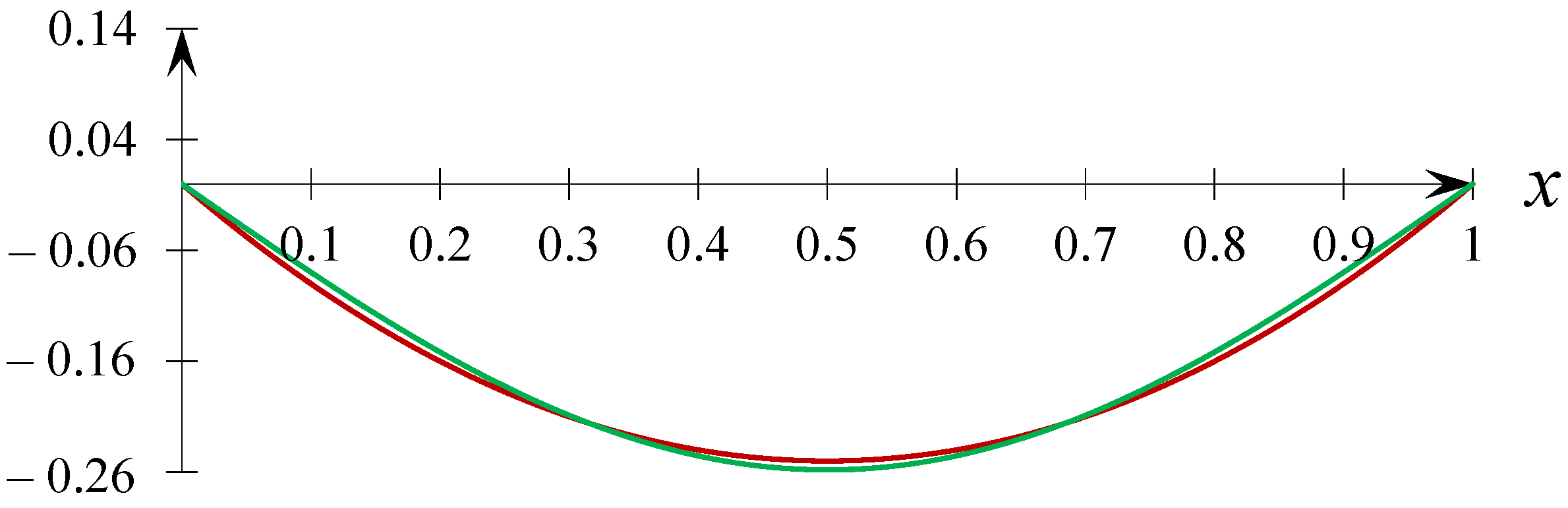
Figure 1 shows the behavior of the obtained function of temperature distribution in the rod.
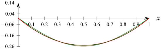
Figure 1.
Graphs of functions (red) and (green).
Table 1 shows the estimation of the deviation of these functions
and comparative analysis of the obtained results.

Table 1.
Deviation estimates for .
Let the material of the rod be copper with a coefficient of thermal diffusivity (25 °C) . Denote , then, we have:
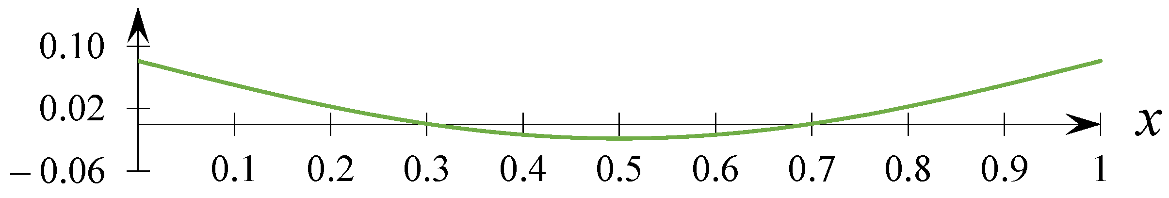
Figure 2 and Figure 3 show the behavior of the obtained function of temperature distribution in the rod.

Figure 2.
Graphs of functions (red) and (green).
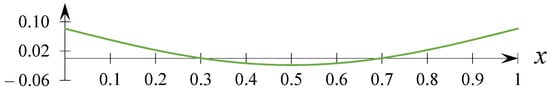
Figure 3.
Graphs of functions and (green).
Table 2 shows the deviation estimate of these functions:
and a comparative analysis of the obtained results for copper.
Table 2.
Deviation estimates for .
Let now the material of the rod be iron with thermal diffusivity . Denote , then, we have:
As can be seen from the formulas obtained at the end of Section 5, the difference between the corresponding formulas for copper and iron materials is only in the value .
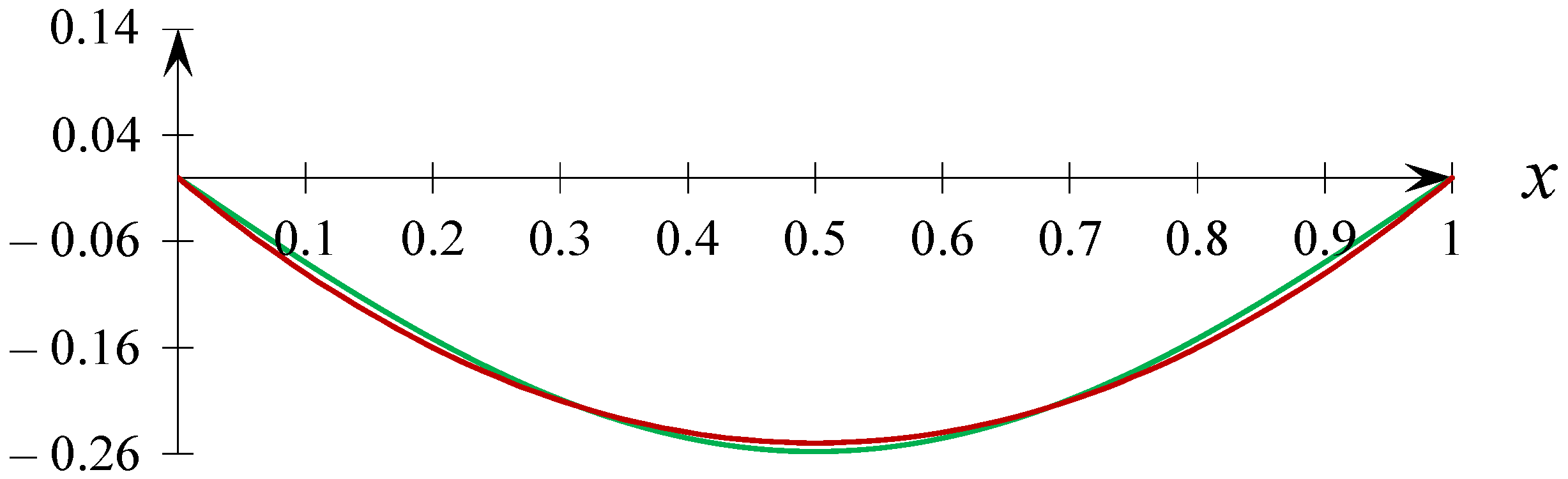
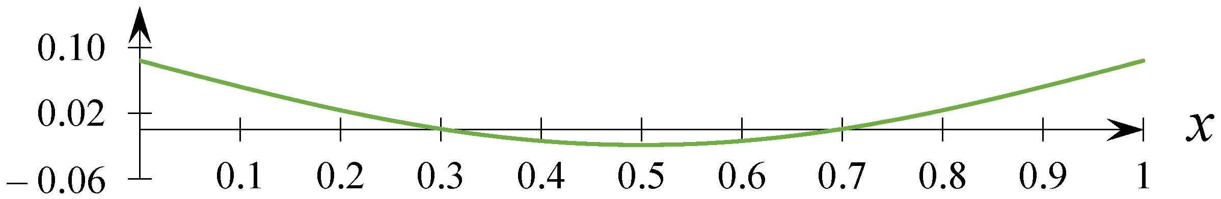
Figure 4 shows the behavior of the obtained function of temperature distribution in the rod.
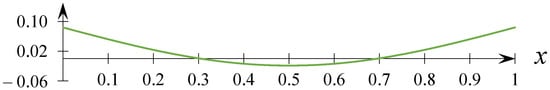
Figure 4.
Graphs of functions and (green).
Table 3 shows the deviation estimate of these functions:
and a comparative analysis of the obtained results for iron.
Table 3.
Deviation estimates for .
Thus, the analysis of the results of the computational experiment confirms the following regularity of the physical properties of the rod material: the lower the thermal diffusivity of the material, the more time is required for boundary control, which provides the desired deviation .
So, using the proposed approach, given , we have constructed explicit expressions of the thermal process control function solving the problem stated above and the explicit expression of the corresponding rod temperature distribution function.
7. Conclusions
For a rod with an insulated side surface, we have proposed a constructive approach to building a function of such temperature conditions at the ends of the rod that change the distribution of the temperature state in the rod from a given initial state to a final state within a given time interval. The proposed approach relies on the method of separation of variables and methods of the theory of control of finite-dimensional systems. With the aid of the Fourier method, the proposed approach can be applied to constructing control of thermal conditions for other non-uniform thermal processes. This attests to the practical significance of the results obtained. The results obtained can be used in the design of boundary control of thermal processes.
Author Contributions
Conceptualization, V.B.; methodology, V.B.; software, S.S.; validation, V.B. and S.S.; formal analysis, V.B. and S.S.; investigation, V.B. and S.S.; resources, V.B. and S.S.; data curation, V.B. and S.S.; writing—original draft preparation, V.B. and S.S.; writing—review and editing, V.B. and S.S.; visualization, V.B. and S.S.; supervision, V.B. and S.S.; project administration, V.B. and S.S.; funding acquisition, V.B. and S.S. All authors have read and agreed to the published version of the manuscript.
Funding
The research by S.S. was carried out under State Assignment Project (no. FWEU-2021-0006) of the Fundamental Research Program of the Russian Federation 2021–2030 using the resources of the High-Temperature Circuit Multi-Access Research Center (Ministry of Science and Higher Education of the Russian Federation, project no 13.CKP.21.0038).
Data Availability Statement
Not applicable.
Conflicts of Interest
The authors declare no conflict of interest. The funders had no role in the design of the study; in the collection, analyses, or interpretation of data; in the writing of the manuscript; or in the decision to publish the results.
References
- Butkovsky, A.G. Control Methods for Systems with Distributed Parameters; Nauka: Moscow, Russia, 1975. (In Russian) [Google Scholar]
- Butkovsky, A.G.; Maly, S.A.; Andreev, Y.N. Optimal Control of Metal Heating; Metallurgiya: Moscow, Russia, 1972. (In Russian) [Google Scholar]
- Egorov, A.I. Optimal Control of Thermal and Diffusion Processes; Nauka: Moscow, Russia, 1978. (In Russian) [Google Scholar]
- Rapoport, E.Y. Structural Modeling of Control Objects and Control Systems with Distributed Parameters; Vysshaya Shkola: Moscow, Russia, 2003. (In Russian) [Google Scholar]
- Tikhonov, A.N.; Samarskii, A.A. Equations of Mathematical Physics; Pergamon Press Ltd.: Oxford, UK, 1963. [Google Scholar]
- Ukhobotov, V.I.; Izmestiev, I.V. The problem of controlling the process of heating of a rod with the unknown temperature at the right end and the unknown density of the heat source. Tr. Inst. Mat. I Mekh. UrO RAN 2019, 25, 297–305. (In Russian) [Google Scholar]
- Butyrin, V.I.; Filshtinsky, L.A. Optimal control of the temperature field in a rod with programmed changes of the control zone. Sov. Appl. Mech. 1976, 12, 115–118. (In Russian) [Google Scholar]
- Kopets, M.M. Optimal control of the heating process of a thin rod. Rep. Natl. Acad. Sci. Ukr. 2014, 7, 48–52. (In Russian) [Google Scholar]
- Gibkina, N.V.; Podusov, D.Y.; Sidorov, M.V. Optimal control of the finite temperature state of a homogeneous rod. Radioelectron. Inform. 2014, 2, 9–15. (In Russian) [Google Scholar]
- Liu, J.; Zheng, G.; Ali, M.M. Stability analysis of the anti-stable heat equation with uncertain disturbance on the boundary. J. Math. Anal. Appl. 2015, 428, 1193–1201. [Google Scholar]
- Dai, J.; Ren, B. UDE-based robust boundary control of heat equation with unknown input disturbance. IFAC Pap. 2017, 50, 11403–11408. [Google Scholar]
- Bonnans, J.F.; Jaisson, P. Optimal control of a parabolic equation with time-dependent state constraints. SIAM J. Control Optim. Soc. Ind. Appl. Math. 2010, 48, 4550–4571. [Google Scholar]
- Lapin, A.; Laitinen, E. Iterative Solution of Mesh Constrained Optimal Control Problems with Two-Level Mesh Approximations of Parabolic State Equation. J. Appl. Math. Phys. 2018, 6, 58–68. [Google Scholar]
- Kunisch, K.; Wang, L. Time optimal control of the heat equation with pointwise control constraints. ESAIM Control. Optim. Calc. Var. 2013, 19, 460–485. [Google Scholar]
- Lemos, J.M.; Marreiro, L.; Costa, B. Supervised multiple model adaptive control of a heating fan. Arch. Control Sci. 2008, 18, 5–16. [Google Scholar]
- Barseghyan, V.R. The problem of control of rod heating process with nonseparated conditions at intermediate moments of time. Arch. Control Sci. 2021, 31, 481–493. [Google Scholar]
- Barseghyan, V.R. Control of Stage by Stage Changing Linear Dynamic Systems. Yugosl. J. Oper. Res. 2012, 22, 31–39. [Google Scholar]
- Barseghyan, V.R.; Barseghyan, T.V. On an Approach to the Problems of Control of Dynamic System with Nonseparated Multipoint Conditions. Autom. Remote Control 2015, 76, 549–559. [Google Scholar]
- Zubov, V.I. Lectures on Control Theory; Nauka: Moscow, Russia, 1975. (In Russian) [Google Scholar]
Disclaimer/Publisher’s Note: The statements, opinions and data contained in all publications are solely those of the individual author(s) and contributor(s) and not of MDPI and/or the editor(s). MDPI and/or the editor(s) disclaim responsibility for any injury to people or property resulting from any ideas, methods, instructions or products referred to in the content. |
© 2023 by the authors. Licensee MDPI, Basel, Switzerland. This article is an open access article distributed under the terms and conditions of the Creative Commons Attribution (CC BY) license (https://creativecommons.org/licenses/by/4.0/).