Inference Based on the Stochastic Expectation Maximization Algorithm in a Kumaraswamy Model with an Application to COVID-19 Cases in Chile

Abstract

Extensive research has been conducted on models that utilize the Kumaraswamy distribution to describe continuous variables with bounded support. In this study, we examine the trapezoidal Kumaraswamy model. Our objective is to propose a parameter estimation method for this model using the stochastic expectation maximization algorithm, which effectively tackles the challenges commonly encountered in the traditional expectation maximization algorithm. We then apply our results to the modeling of daily COVID-19 cases in Chile.

1. Introduction

The Kumaraswamy distribution [1], originally referred to as the double-bounded model, was introduced to describe hydrological data. Later, in [2], it was renamed the Kumaraswamy distribution. Additional references to this and related distributions include [3,4,5,6,7,8,9,10,11,12,13,14,15,16]. Recently, the trapezoidal Kumaraswamy (TK) distribution [17] was developed to enhance the flexibility of the Kumaraswamy distribution while preserving its fundamental properties. To offer more versatility than their base models, several extensions of the Kumaraswamy distribution have been proposed, such as the Kumaraswamy-Weibull [18], Kumaraswamy–Fréchet [19], and Kumaraswamy-generalized gamma [20] distributions. However, these extensions do not allow for the modeling of tail-area events. In cases where heavy left- and right-tailed distributions are required for modeling bounded data, neither the beta nor Kumaraswamy distributions, including the aforementioned extensions, are suitable, as noted in [21,22]. To address this unsuitability, the TK distribution was introduced in [17], adding flexibility to the beta and Kumaraswamy distributions.

The TK distribution is a mixture model that enables the modeling of bounded data with heavy tails in different proportions in these tails. Here, we leverage the finite mixture representation of the TK distribution to implement the expectation- maximization (EM) algorithm. The EM algorithm, which consists of an expectation (E) step and a maximization (M) step, is widely used for iterative computation of maximum likelihood estimates, particularly in missing data settings. In the context of mixture models, the EM algorithm assumes that the mixture arises from missing observations. Further details about this algorithm can be found in [23]. The EM algorithm, introduced in [24], has been extensively applied in various contexts. For more specific information on these contexts, readers may refer to [25,26,27,28,29,30,31,32,33].

The maximization step of the EM algorithm can encounter problems, especially when dealing with multimodal likelihood functions [34]. To address these problems, as well as others discussed in subsequent sections, an alternative approach called the stochastic expectation maximization (SEM) algorithm was proposed in [35], employing a Bayesian framework. The SEM algorithm introduces an additional stage known as the S-step, which involves simulation methods such as Gibbs sampling and the Metropolis–Hastings algorithm to obtain posterior distributions of the parameters. By incorporating prior information and utilizing it to overcome the problems encountered in the EM approach, the SEM algorithm offers a solution. By properly rewriting the TK distribution as a mixture model, we can utilize the SEM algorithm to estimate its parameters. To the best of our knowledge, this approach to estimating the parameters of the TK distribution has not previously been considered.

Modeling bounded data is a widely discussed topic in the literature, particularly in relation to statistical indicators such as mortality rates, recovery rates, economic measures, and risk measures [36]. In various fields of research, continuous variables expressed as proportions, rates, ratios, and indices pose challenges. During the COVID-19 pandemic, this type of information was crucial for investigating issues related to infected cases, recovered cases, and deaths worldwide [37,38]. The emergence of severe acute respiratory syndrome coronavirus 2 (SARS-CoV-2) in December 2019 caused a global state of confusion as governments strove to monitor and control the disease without prior information [39,40]. In this paper, we apply our results to COVID-19 data. The impact of the pandemic extended beyond public health, affecting aspects such as the economy and gross domestic product, especially in Latin America [41]. Different models have proven to be relevant in forecasting epidemic diseases, and various methodologies have been employed to gain insights into diverse aspects of epidemics around the world [42,43,44,45,46,47,48,49,50,51,52,53,54,55,56,57,58,59,60].

The objectives of this investigation are twofold: (i) to propose an estimation method for the parameters of the TK distribution based on the SEM algorithm, and (ii) to apply the obtained results to the modeling of daily COVID-19 cases in Chile. We implemented the obtained results in the R software [61].

The remainder of this article is organized as follows. Section 2 presents a general overview of the TK distribution and of the EM algorithm applied to mixture models. In Section 3, we describe how the SEM algorithm is implemented for the TK model and highlight its main differences with the EM algorithm. First, we treat the parameters as random variables, leveraging the prior information available about them. Second, we utilize joint prior distributions and simulate the parameters from their posterior distribution using Gibbs sampling and the Metropolis–Hastings algorithm. Next, Section 4 demonstrates the functionality of the SEM algorithm using 100 datasets across different scenarios. In Section 5, we apply our results to a real-world dataset concerning daily COVID-19 cases in Chile. Finally, Section 6 concludes the article by providing insights into our findings.

2. Background

In this section, we describe preliminary aspects of the TK distribution and EM algorithm.

2.1. Trapezoidal Kumaraswamy Distribution

A random variable Y follows a TK distribution with parameters ${\Theta }^{\prime }={(a,b,\alpha ,\beta )}^{\top }={(a,b,{\Theta }^{\top })}^{\top }$, that is, $\Theta ={(\alpha ,\beta )}^{\top }$, if its probability density function (PDF) is provided by

$$f_{\mathrm{TK}}(y;a,b,\alpha ,\beta )=a+(b-a)y+\left(1-\frac{a+b}{2}\right)f_{\mathrm{K}}(y;\alpha ,\beta ),y\in (0,1),$$

(1)

where $0\le a,b\le 2,a+b\le 2$, and $f_{\mathrm{K}}$ is the Kumaraswamy PDF [1] with parameters $\alpha ,\beta >0$. As an example, Figure 1 shows shapes of the TK PDF defined in (1).

The expected value and variance of the TK distribution are formulated as $\mathrm{E}\left(Y\right)=m_1$ and $\mathrm{Var}\left(Y\right)=m_2-m_1^2$, where $m_k$ denotes the k-th moment of the TK distribution, that is,

$$m_k=\frac{a}{k+1}+\frac{b-a}{k+2}+\left(1-\frac{a+b}{2}\right)\beta B\left(1+\frac{k}{\alpha },\beta \right),$$

where $B(c,d)$ is the beta function in terms of c and d.

2.2. EM Algorithm

The EM algorithm is a general method for finding maximum likelihood estimates when there are missing values or latent variables. It can be used for mixture models based on an observed data set of a random variable Y that is classified as a mixture component according to a probability. The basic idea behind this algorithm is the assumption that the dataset results from an unobservable discrete random variable U, which indicates the mixture component that generated observation $y_i$ and allows us to fit these probabilities in each iteration until a convergence criterion is reached.

Next, we describe the general steps of the EM algorithm for estimating the TK parameters ${\Theta }^{\prime }$. For each variable $Y_i$, with $i\in \{1,\dots ,n\}$ and n denoting the sample size, ${\mathit{U}}_i={(U_{i1},U_{i2},U_{i3})}^{\top }$ is the discrete random vector indicating to which mixture component $Y_i$ belongs, that is, $U_{ij}=1$ if $Y_i$ belongs to class j and $U_{ij}=0$ otherwise, for $j\in \{1,2,3\}$. Note that $\mathit{y}={(y_1,\dots ,y_n)}^{\top }$ is the vector of the observed data associated with the random vector $\mathit{Y}={(Y_1,\dots ,Y_n)}^{\top }$; $\mathit{u}={({\mathit{u}}_1,\dots ,{\mathit{u}}_n)}^{\top }$ is the matrix of unobserved (missing) data related to $\mathit{U}={({\mathit{U}}_1,\dots ,{\mathit{U}}_n)}^{\top }$; and $\mathit{z}={({\mathit{z}}_1,\dots ,{\mathit{z}}_n)}^{\top }$ is the matrix of complete data regarding $\mathit{Z}={({\mathit{Z}}_1,\dots ,{\mathit{Z}}_n)}^{\top }$, where ${\mathit{Z}}_i=(Y_i,{\mathit{U}}_i)$, for $i\in \{1,\dots ,n\}$. Thus, in our case, the EM algorithm consists of iterating the following steps:

E-step: Compute ${\widehat{U}}_{ij}^{\left(t\right)}$ and parameter estimates from initial values at $t=0$.

M-step: Update the parameters estimates according to ${{\widehat{\Theta }}^{\prime }}^{\left(t\right)}={\mathrm{argmax}}_{{\Theta }^{\prime }}\mathsf{\ell }({{\Theta }^{\prime }}^{(t-1)},\mathit{z})$.

Note that the M-step must be iterated until reaching convergence, where t indexes the t-th iteration, ${\widehat{U}}_{ij}^{\left(t\right)}$ is the probability that observation i comes from component j of the mixture, and ℓ is the log-likelihood function, which is formulated utilizing the three-component mixture structure of the TK distribution; see more details in [62].

Unfortunately, as mentioned, the EM algorithm has some problems, including its dependence on initial values for the case of multimodal likelihood functions that may produce saddle points [62] and slow convergence in several other cases [34]. To avoid these problems, several extensions of the EM algorithm have been proposed, including those based on Bayesian approaches, with the SEM algorithm being one of these extensions. Note that a good EM algorithm should converge to the true maximization point. For details regarding the usual EM algorithm, see [23]. In Section 3, we provide further necessary details to deal with the SEM algorithm, which as mentioned is a very popular extension of the EM algorithm used to estimate mixture model parameters.

3. Bayesian Estimation for the Trapezoidal Kumaraswamy Model

In this section, we describe how to efficiently estimate the parameters of the TK distribution using the SEM algorithm.

3.1. The Model

As mentioned in Section 2.2, the EM algorithm and its variants require the model to be represented as a mixture of PDFs. To satisfy this requirement, we can rewrite the PDF stated in (1) as

$$f_{\mathrm{TK}}(y;a,b,\alpha ,\beta )=\frac{a}{2}(2-2y)+\frac{b}{2}\left(2y\right)+\left(1-\frac{a+b}{2}\right)f_{\mathrm{K}}(y;\alpha ,\beta ),$$

(2)

where $f_1\left(y\right)=f_{\mathrm{B}}(y;1,2)=2-2y$ and $f_2\left(y\right)=f_{\mathrm{B}}(y;2,1)=2y$ are the PDFs of the beta distribution denoted as $f_{\mathrm{B}}$. Then, the PDF stated in (2) can be expressed in a mixture form as

$$f_{\mathrm{TK}}(y;a,b,\alpha ,\beta )=w_1{f}_{\mathrm{B}}(y;1,2)+w_2{f}_{\mathrm{B}}(y;2,1)+w_3{f}_{\mathrm{K}}(y;\alpha ,\beta ),$$

with $w_1=a/2$, $w_2=b/2$, and $w_3=1-\left(a+b\right)/2$ representing the weights of each PDF in the mixture model, where $0\le w_j\le 1$ and ${\sum }_{j=1}^3{w}_j=1$, for $j\in \{1,2,3\}$. Therefore, the parameters to be estimated in this model are now ${\Theta }^{★}={(\mathit{w},\Theta )}^{\top }$, where $\mathit{w}={(w_1,w_2,w_3)}^{\top }$ and, as earlier defined, $\Theta ={(\alpha ,\beta )}^{\top }$.

As in the EM framework, the SEM algorithm requires the model to be a mixture and to be expressed in terms of missing data. Thus, for each variable $Y_i$, with $i\in \{1,\dots ,n\}$, ${\mathit{U}}_i=(U_{i1},U_{i2},U_{i3})$ is a vector indicating to which mixture component $Y_i$ belongs, that is,

$$U_{ij}=\left\{\begin{array}{cc}1,& \mathrm{if}{Y}_i\mathrm{belongs}\mathrm{to}\mathrm{component}j;\\ 0,& \mathrm{otherwise}.\end{array}\right.$$

Recall that $\mathit{y}={(y_1,\dots ,y_n)}^{\top }$ is the vector of observed data associated with $\mathit{Y}={(Y_1,\dots ,Y_n)}^{\top }$; $\mathit{u}={({\mathit{u}}_1,\dots ,{\mathit{u}}_n)}^{\top }$ is the matrix of unobserved (missing) data related to $\mathit{U}={({\mathit{U}}_1,\dots ,{\mathit{U}}_n)}^{\top }$; and $\mathit{z}={(z_1,\dots ,z_n)}^{\top }$ is the matrix of complete data regarding $\mathit{Z}={({\mathit{Z}}_1,\dots ,{\mathit{Z}}_n)}^{\top }$, where ${\mathit{Z}}_i=(Y_i,{\mathit{U}}_i)=(Y_i,U_{i1},U_{i2},U_{i3})$, for $i\in \{1,\dots ,n\}$. Then, the likelihood function for the complete data $\mathit{z}={(\mathit{y},\mathit{u})}^{\top }$ is provided by

$$L({\Theta }^{★};\mathit{z})=\prod _{i=1}^n\prod _{j=1}^3{\left(w_j{f}_j(y_i;{\mathit{\theta }}_j)\right)}^{u_{ij}},$$

(3)

and the log-likelihood function obtained from (3) is stated as

$$\mathsf{\ell }({\Theta }^{★};\mathit{z})=\sum _{j=1}^3\sum _{i=1}^n{u}_{ij}log\left(w_j{f}_j(y_i;{\mathit{\theta }}_j)\right),$$

with $f_1(y_i;{\mathit{\theta }}_1)=f_{\mathrm{B}}(y_i;1,2)$, $f_2(y_i;{\mathit{\theta }}_2)=f_{\mathrm{B}}(y_i;2,1)$, and $f_3(y_i;{\mathit{\theta }}_3)=f_{\mathrm{K}}(y;\alpha ,\beta )$.

3.2. SEM Algorithm

Next, we describe the step-by-step application of the SEM algorithm to the TK model from initial values for ${\Theta }^{★}$, that is, for $t=0$, we have ${\mathit{w}}^{\left(0\right)}={(w_1^{\left(0\right)},w_2^{\left(0\right)},w_3^{\left(0\right)})}^{\top }$ and ${\Theta }^{\left(0\right)}={({\alpha }^{\left(0\right)},{\beta }^{\left(0\right)})}^{\top }$.

E-step:

As $U_{ij}$ represents each observed item of data belonging to certain mixture components of the model, we can estimate its value based on its expectation [23], that is, we must compute the probability formulated as

$${\widehat{U}}_{ij}^{\left(t\right)}=P\left(U_{ij}=1|Y_i=y_i\right){|}_{{\Theta }^{★}={\Theta }^{★(t-1)}}=\frac{w_j^{(t-1)}{f}_j\left(y_i\right|{\alpha }^{(t-1)},{\beta }^{(t-1)})}{{\sum }_{l=1}^3{w}_l^{(t-1)}{f}_l\left(y_i\right|{\alpha }^{(t-1)},{\beta }^{(t-1)})},i\in \{1,\dots ,n\},j\in \{1,2,3\}.$$

(4)

In practical terms, ${\widehat{U}}_{ij}^{\left(t\right)}$ in step t is the posterior probability of observation i arising from component j of the model, evaluated at the values in a previous iteration $t-1$, which we denote by ${|}_{{\Theta }^{★}={\Theta }^{★(t-1)}}$.

S-step:

As mentioned, the EM algorithm can present problems after the E-step in the case of multimodal likelihood functions, which imply dependence on initial conditions without a guaranteed local maximum, in addition to presenting possible saddle points, as mentioned in Section 2.2. To solve these problems, we propose using a Bayesian approach. In particular, the complete data $\mathit{z}={(\mathit{y},\mathit{u})}^{\top }$, whose joint PDF is denoted in general by f, can be combined with prior information about the parameters ${\Theta }^{★}$. That is, we can assign a prior probability distribution with PDF $\pi ({\Theta }^{★})$ that, according to the Bayes theorem, is stated as

$$\pi ({\Theta }^{★}|\mathit{z})=\frac{f(\mathit{z}|{\Theta }^{★})\pi ({\Theta }^{★})}{{\int }_{S_{{\Theta }^{★}}}f(\mathit{z}|{\Theta }^{★})\pi ({\Theta }^{★})\mathrm{d}{\Theta }^{★}}\propto f(\mathit{z}|{\Theta }^{★})\pi ({\Theta }^{★}),$$

(5)

which implies that we can know the posterior distribution for each unknown parameter, with $S_{{\Theta }^{★}}$ being the support of ${\Theta }^{★}$, recalling that ${\Theta }^{★}={(w_1,w_2,w_3,\alpha ,\beta )}^{\top }$. The inclusion of the S-step of the SEM algorithm may be considered a Bayesian extension of the usual EM algorithm, as it consists of simulating $\mathit{U}$, $\mathit{W}$, and ${\Theta }^{★}$ from their posterior distributions, as indicated in (5). As described below, the simulation techniques we use here are the Gibbs sampling and Metropolis–Hastings algorithm [63].

In the S-step, we simulate $U_{ij}$ from its posterior distribution, which we can assume intuitively to be multinomially distributed and have a size equal to one with probabilities $({\widehat{U}}_{i1},{\widehat{U}}_{i2},{\widehat{U}}_{i3})$. Therefore, in the t-th iteration, $U_i^{\left(t\right)}\sim \mathcal{M}(1;{\widehat{U}}_{i1}^{\left(t\right)},{\widehat{U}}_{i2}^{\left(t\right)},{\widehat{U}}_{i3}^{\left(t\right)})$. This provides a vector with a one in its components and two other vectors with zeros, that is, the data are assigned randomly to a component with a value of one.

The M-step of the SEM algorithm depends on the form of the PDF, and its solution often does not exist in closed form. In addition, it is possible that the values of the parameters to become too large during the iterations, causing a numerical problem [62]. To avoid this problem, a viable approach could be simulating the parameters instead computing them. According to [64], this approach is one of the most widely used in Bayesian estimation for mixture models. The association of each observation $y_i$ with an unobservable data ${\mathit{u}}_i$ allows us to simulate $W_j$ from its posterior distribution $\pi \left(\mathit{w}\right|\mathit{u})$. Observe that $\mathit{W}$ is independent of $\mathit{Y}$, that is, $\pi \left(\mathit{w}\right|\mathit{y},\mathit{u})=\pi (\mathit{w}\left|\mathit{u}\right)$. The standard Gibbs sampler for mixture models is based on successive simulations of $\mathit{U}$, $\mathit{W}$, and ${\Theta }^{★}$.

We know that $\pi \left(\mathit{w}\right|\mathit{u})\propto \pi (\mathit{u}\left|\mathit{w}\right)\pi \left(\mathit{w}\right)$. Then, given the known prior information, we have $\mathit{w}={(w_1,w_2,w_3)}^{\top }$, for $0<w_j<1$, and ${\sum }_{j=1}^3{w}_j=1$. Thus, it is intuitive to assume that $\mathit{W}$ is Dirichlet distributed, that is, we have

$$\pi \left(\mathit{w}\right)=\frac{\Gamma \left({\sum }_{j=1}^3{\eta }_j\right)}{{\prod }_{j=1}^3\Gamma \left({\eta }_j\right)}\prod _{j=1}^3{w}_j^{{\eta }_j-1},$$

(6)

where $\Gamma$ is the usual gamma function and $\mathit{\eta }={({\eta }_1,{\eta }_2,{\eta }_3)}^{\top }$ is the parameter vector of the Dirichlet distribution. In addition, we have

$$\pi \left(\mathit{u}\right|\mathit{w})=\prod _{i=1}^n\pi \left(u_i\right|\mathit{w})=\prod _{i=1}^n{w}_1^{u_{i1}}{w}_2^{u_{i2}}{w}_3^{u_{i3}}=\prod _{i=1}^n\prod _{j=1}^3{w}_j^{u_{ij}}=\prod _{j=1}^3{w}_j^{n_j},$$

(7)

where $n_j={\sum }_{i=1}^n{\mathbb{1}}_{u_{ij}=1}$ is the number of observations assigned to component j in the S-step, with ${\mathbb{1}}_B$ being the indicator function in the set B. This means that each $n_j$ is the sum of each $u_{ij}=1$ simulated from $U_{ij}$ in each iteration. Then, by assembling both of the equations stated in (6) and (7), we can prove that

$$\pi \left(\mathit{w}\right|\mathit{u})\propto \mathcal{D}({\eta }_1+n_1,{\eta }_2+n_2,{\eta }_3+n_3),$$

(8)

where $\mathcal{D}$ is the Dirichlet PDF with parameters $({\eta }_1+n_1,{\eta }_2+n_2,{\eta }_3+n_3)$. Note that ${\eta }_1$, ${\eta }_2$, and ${\eta }_3$ are hyperparameters. To estimate the parameters of the Kumaraswamy distribution, that is, $\Theta ={(\alpha ,\beta )}^{\top }$, we must simulate them from the joint posterior distribution $\pi ({\Theta }^{\left(t\right)}|{\mathit{u}}^{\left(t\right)},\mathit{y})=\pi ({\alpha }^{\left(t\right)},{\beta }^{\left(t\right)}|{\mathit{u}}^{\left(t\right)},\mathit{y})$. To do it, we use the Metropolis–Hastings algorithm whose steps are:

(i)

Generate candidates ${\alpha }^{*},{\beta }^{*}$ from

$$\begin{array}{cc}\hfill {\alpha }^{*}& \sim \mathcal{LN}\left(log({\alpha }^{(t-1)}),{\sigma }^2\right),\end{array}$$

(9)

$$\begin{array}{cc}\hfill {\beta }^{*}& \sim \mathcal{LN}\left(log({\beta }^{(t-1)}),{\sigma }^2\right),\end{array}$$

(10)

where $\sigma$ is a hyperparameter and $\mathcal{LN}$ denotes the log-normal distribution. Here, we know that

$$\pi ({\alpha }^{*},{\beta }^{*}|{\mathit{u}}^{\left(t\right)},\mathit{y})\propto \pi (\mathit{y},{\mathit{u}}^{\left(t\right)}|{\alpha }^{*},{\beta }^{*})\pi ({\alpha }^{*},{\beta }^{*})=\left(\prod _{i=1}^n{\left(f_{\mathrm{TK}}(y_i;2w_1,2w_2,\alpha ,\beta |{\alpha }^{*},{\beta }^{*})\right)}^{{\mathbb{1}}_{u_{i3}=1}}\right)\pi \left({\alpha }^{*}\right)\pi \left({\beta }^{*}\right).$$

Then, with probability $\delta$ provided by

$$\delta \left(\left.\begin{array}{c}\left(\begin{array}{c}{\alpha }^{*}\\ {\beta }^{*}\end{array}\right)\end{array}\right|\left(\begin{array}{c}{\alpha }^{(t-1)}\\ {\beta }^{(t-1)}\end{array}\right)\right)=min\left\{1,\frac{\pi ({\alpha }^{*},{\beta }^{*}|{\mathit{u}}^{\left(t\right)},\mathit{y})}{\pi ({\alpha }^{(t-1)},{\beta }^{(t-1)}|{\mathit{u}}^{\left(t\right)},\mathit{y})}\right\},$$

(11)

we accept or reject the new values of the parameters (both of them).

(ii)

For a value $v^{*}$ generated from $V^{*}\sim {\mathcal{U}}_{[0,1]}$, that is, uniform in [0, 1], consider

$$\left(\begin{array}{c}{\alpha }^{\left(t\right)}\\ {\beta }^{\left(t\right)}\end{array}\right)=\left\{\begin{array}{cc}\left(\begin{array}{c}{\alpha }^{*}\\ {\beta }^{*}\end{array}\right),& \mathrm{if}\delta \ge v^{*},\\ \left(\begin{array}{c}{\alpha }^{(t-1)}\\ {\beta }^{(t-1)}\end{array}\right),& \mathrm{if}\delta <v^{*}.\end{array}\right.$$

(12)

In summary, the application of the SEM algorithm to the TK model must consider the following:

(i)

[Initialization] Set arbitrary initial values for the parameter vector $\Theta ={\Theta }^{\left(0\right)}$.

(ii)

[E-step] Compute ${\widehat{U}}_{ij}^{\left(t\right)}$ from (4).

(iii)

[S-step] Simulate a sample from $U_i^{\left(t\right)}\sim \mathcal{M}(1;{\widehat{U}}_{i1}^{\left(t\right)},{\widehat{U}}_{i2}^{\left(t\right)},{\widehat{U}}_{i3}^{\left(t\right)})$ for each $Y_i$.

(iv)

[M-step]

(a)

Establish the weights from $W^{\left(t\right)}\sim \mathcal{D}({\eta }_1+n_1^{\left(t\right)},{\eta }_2+n_2^{\left(t\right)},{\eta }_3+n_3^{\left(t\right)})$.

(b)

Generate the candidates $({\alpha }^{*},{\beta }^{*})$ from (9) and (10).

(c)

Calcalute $\delta$ from (11), generate $v^{*}$ from $V^{*}\sim \mathcal{U}[0,1]$ and accept or reject $({\alpha }^{*},{\beta }^{*})$ according to (12).

(v)

[Iteration] Repeat E-step, S-step, and M-step until a convergence criterion is achieved.

4. Simulation Study

In this section, we perform a simulation study to compare the performance of the TK distribution under different scenarios. First, we present a brief discussion on the value of ${\sigma }^2$ and the hyperparameters ${\eta }_l$ for $l\in \{1,2,3\}$. Then, we compare the performance of the TK and Kumaraswamy distributions for samples generated from each of them.

4.1. Simulation Scenario

It can be observed that the parameters ${\alpha }^{*}$ and ${\beta }^{*}$ have been generated from the log-normal distribution with variance ${\sigma }^2$. Hence, the variance of ${\alpha }^{*}$ is equal to $(exp\left({\sigma }^2\right)-1)exp(2log\left({\alpha }^{(t-1)}\right)+{\sigma }^2)$, and assigning a value to the hyperparameter ${\sigma }^2$ should be done cautiously. For example, if we consider $log\left({\alpha }^{(t-1)}\right)=5$ and a standard deviation $\sigma =0.5$ and $1.0$, then $\mathrm{Var}\left({\alpha }^{*}\right)=8032.96$ and 102,880.6, respectively. Thus, a value of the hyperparameter $\sigma =1.0$ may seem extremely high for exploring a new updated ${\alpha }^{*}$, such as that noted in Section 4.2 (analogous to ${\beta }^{*}$). In addition, from (8), we have $w^{\left(t\right)}\propto \mathcal{D}({\eta }_1+n_1^{\left(t\right)},{\eta }_2+n_2^{\left(t\right)},{\eta }_3+n_3^{\left(t\right)})$, where $n_j$ is the total amount of data assigned to component j. Hence, we suppose that the hyperparameters ${\eta }_i$, for $i\in \{1,2,3\}$, can take, for example, values ${\eta }_i=0.1$ or $1.0$ indistinctly. In fact, if we have lifted tails in the distribution, both values achieve good results. However, if the tails are not lifted, then, when ${\eta }_i=0.1$, the estimates of a and b are closer to zero, as noted in the Kumaraswamy simulation of Section 4.2. All the numerical calculations were obtained considering 100,000 Monte Carlo replicates and discarding the first 40,000 as burn-in.

To capture each tail behavior in the TK distribution, we generated 100 samples of size 1000 to compute the average deviance information criterion (DIC) proposed in [65], the expected Akaike information criterion (EAIC) introduced in [66], and the expected Bayesian information criterion (EBIC) provided in [67]. First, we ran the simulation using the TK distribution with ${\Theta }^{\prime }={(0.1,0.3,5,10)}^{\top }$, allowing us to model a skewed distribution with independently lifted tails, which captures the essence of the TK distribution. Second, we used a sample from the Kumaraswamy distribution with the parameters provided by ${(a,b)}^{\top }={(5,10)}^{\top }$, that is, a skewed distribution that lacks lifted tails in its PDF.

4.2. Results of the Simulations

For the first simulation using the TK distribution, it can be concluded from

Table 1. Values of the mean DIC, EAIC, and EBIC in the indicated distribution for 100 samples of size 1000 generated from a TK distribution with parameters $(0.1,0.3,5,10)$.

Distribution	$(\mathit{\sigma },{\mathit{\eta }}_{\mathit{i}})$	Mean DIC	Mean EAIC	Mean EBIC
TK	(0.5, 0.1)	−802.301	−794.466	−774.835
	(0.5, 1)	−801.519	−794.616	−774.985
	(1, 0.1)	−780.712	−782.756	−763.125
	(1, 1)	−783.543	−783.138	−763.507
Kumaraswamy	$\sigma =0.5$	−526.796	−604.993	−595.177

that the TK distribution obtains a better fit than the Kumaraswamy distribution. Note that the value of the hyperparameter $\sigma$ must be chosen carefully, as mentioned, providing better results when $\sigma =0.5$, as stated in Section 4.1. In

Table 2. Estimated posterior medians, means, and credibility intervals (CI) for 100 samples of size 1000 generated from a TK distribution with parameters $(0.1,0.3,5,10)$.

Distribution	Parameter	True Value	Mean	Standard Deviation	Median	95% CI
TK	a	0.1	0.098	0.018	0.095	(0.077, 0.117)
	b	0.3	0.300	0.027	0.298	(0.263, 0.335)
	$\alpha$	5	4.944	0.271	4.933	(4.637, 5.237)
	$\beta$	10	9.932	1.234	9.646	(8.303, 11.233)
Kumaraswamy	$\alpha$	-	3.006	0.154	2.996	(2.828, 3.170)
	$\beta$	-	3.139	0.327	3.097	(2.825, 3.398)

, we consider results from the TK distribution with hyperparameters $\sigma =0.5$ and ${\eta }_i=0.1$, as well as from the Kumaraswamy distribution. It is noteworthy that the Kumaraswamy distribution attempts to fit the model by increasing the variance, that is, by selecting small values for $\alpha$ and $\beta$, to compensate for its inability to produce lifted tails.

Table 3. Relbias and root squared error of each parameter under 100 samples of size 1000 generated from a TK distribution with parameters $(0.1,0.3,5,10)$.

Indicator	a	b	$\mathit{\alpha }$	$\mathit{\beta }$
RelBias	−0.0041	−0.0283	−0.0174	−0.0231
$\mathrm{RMSE}$	0.0139	0.0212	0.2170	0.9884

presents two statistical indicators: the empirical relative bias (RelBias), and the root mean squared error ($\mathrm{RMSE}$) for each parameter estimator over the 100 simulated samples from the TK distribution. These indicators are defined as

$$\begin{array}{c}\hfill \mathrm{RelBias}\left(\theta \right)=\frac{1}{100}\sum _{i=1}^{100}\left(\frac{{\widehat{\theta }}^{\left(i\right)}-\theta }{\theta }\right)\mathrm{and}\mathrm{MSE}\left(\theta \right)=\frac{1}{100}\sum _{i=1}^{100}{({\widehat{\theta }}^{\left(i\right)}-\theta )}^2,\end{array}$$

where $\theta$ represents a specific parameter of interest and ${\widehat{\theta }}^{\left(i\right)}$ denotes the posterior estimate of $\theta$ obtained from sample i. Table 3 shows that the estimation of each parameter in each dataset is good when the TK distribution is adjusted.

In Table 2, we reported the results of the estimation process for each parameter for both models, where a and b come from $\mathit{w}={(w_1,w_2)}^{\top }$ with $w_1=a/2$ and $w_2=b/2$, according to the definition of the model provided in Section 3.1. Upon conducting the second simulation using the Kumaraswamy distribution, it is evident from

Table 4. Values of the mean DIC, EAIC, and EBIC in the indicated distribution for 100 samples of size 1000 generated from a Kumaraswamy distribution with parameters $(5,10)$.

Distribution	($\mathit{\sigma },{\mathit{\eta }}_{\mathit{i}})$	Mean DIC	Mean EAIC	Mean EBIC
TK	(0.5, 0.1)	−1257.515	−1321.922	−1302.291
	(0.5, 1)	−1232.631	−1311.324	−1291.693
Kumaraswamy	$\sigma =0.5$	−1257.887	−1326.381	−1316.566

that the TK distribution provides an adequate fit, similar to that of the Kumaraswamy distribution. Furthermore,

Table 5. Estimated posterior medians and means for 100 samples of size 1000 drawn from a Kumaraswamy distribution with parameters $(5,10)$.

Distribution	Parameter	True Value	Mean	Standard Deviation	Median	95% CI
TK	a	0	$5.58\times {10}^{-4}$	$4.44\times {10}^{-4}$	$2.65\times {10}^{-5}$	$(3.52\times {10}^{-8}, 6.32\times {10}^{-4})$
	b	0	$7.98\times {10}^{-4}$	$1.24\times {10}^{-3}$	$2.25\times {10}^{-4}$	$(3.04\times {10}^{-5}, 1.12\times {10}^{-3})$
	$\alpha$	5	4.980	0.149	4.970	(4.715, 5.249)
	$\beta$	10	10.054	0.715	9.839	(8.666, 11.272)
Kumaraswamy	$\alpha$	5	4.971	0.152	4.963	(4.709, 5.239)
	$\beta$	10	10.009	0.728	9.804	(8.641, 11.214)

shows that the parameter estimates obtained with the TK distribution are comparable to those obtained from the Kumaraswamy distribution.

When the true values a and b are zero, the hyperparameter ${\eta }_i=0.1$ may be a better option than ${\eta }_i=1$. Then, the hyperparameter combination for $(\sigma ,{\eta }_i)$ equal to $(0.5,0.1)$ provides good results in different scenarios. In summary, it is not surprising that we observe similar values for the mean DIC, EAIC, and EBIC achieved with the Kumaraswamy and TK distributions when the sample is generated from the Kumaraswamy distribution. However, when the sample is generated from a TK distribution with a difference between its two tails ($a=0.1$ and $b=0.3$), the TK distribution achieves the best fit in terms of the mean DIC, EAIC, and EBIC. This result is expected, as the data generated from the tails of the distribution cannot be adequately captured by the Kumaraswamy distribution alone.

5. Empirical Illustration Using Real-World Data

As illustration, the proposed method is applied to real data fitting the TK and Kumaraswamy distributions. The appendix presents the codes used in this illustration.

COVID-19 Data

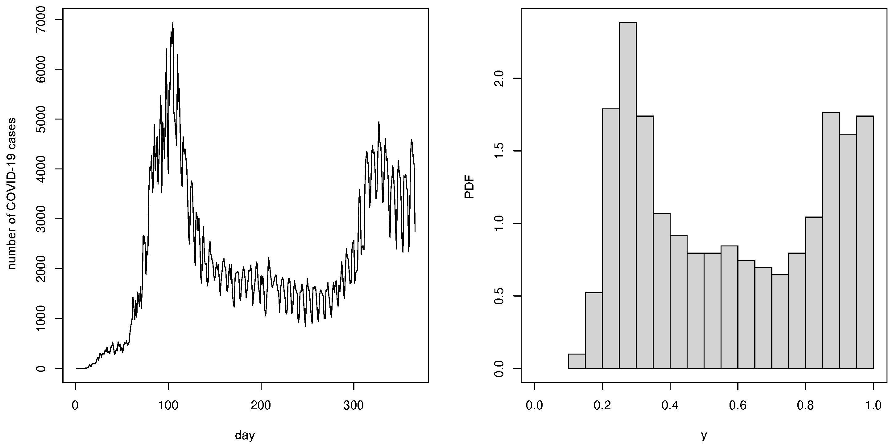
The COVID-19 outbreak and worldwide spread has led to a pandemic. In Figure 2, two peaks are apparent, indicating the first and second massive outbreaks during June 2020 and January 2021. The data that we analyze here contain the number of daily confirmed and probable cases in Chile, from the first detected case on 02 March 2020 to 03 March 2021 (366 records), with each datapoint corresponding to the cases on the previous day. These data are available from the Chilean government under the Ministry of Science, Technology, Knowledge, and Innovation (www.minciencia.gob.cl/covid19; accessed on 21 June 2023).

We fit the TK model to the behavior of data on new daily cases in Chile and compared this with the fit of the Kumaraswamy model. Due to the curve corresponding to a daily measure, we first must transform it into a probability model of a random variable that takes values in (0, 1), with values of zero and one not being included, that is, transforming days 1 to 366 to (0, 1). Then, we consider all new cases for the day on which they were observed and transform them to the value of their proper day. This involves assigning all days a proportional weight according to the number of new cases recorded to obtain the shape and growth of the original data for the TK distribution, resulting in the histogram shown in Figure 2. Therefore, from (13) and following [68], we have

$$\begin{array}{c}\hfill y=\left(\frac{N-1}{N}\right)\left(\frac{y^{*}-a_1}{a_2-a_1}\right)+\frac{1}{2N},y^{*}\in [a_1,a_2].\end{array}$$

(13)

Here, $N=$ 800,569 represents the sum of the all new daily cases, whereas $a_1=1$ and $a_2=366$ are the first and last day of the observations, with $y\in (0,1)$. Now, for each $y_i$ with $i\in \{1,\dots ,366\}$, we repeat its value as many times as needed to indicate the total daily cases. For example, if on the last day (day 366, $y_{366}=0.9999$), there were 2747 new cases, in our sample the value $y_{366}$ is repeated 2747 times. Because the required time in processing the full data set is large, and as the shape of the distribution is not affected, we take only a portion of the total sample, that is, 805 observations. To know which day is represented by the value of any y, we can return from transforming and solve the equation stated in (13) for $y^{*}$.

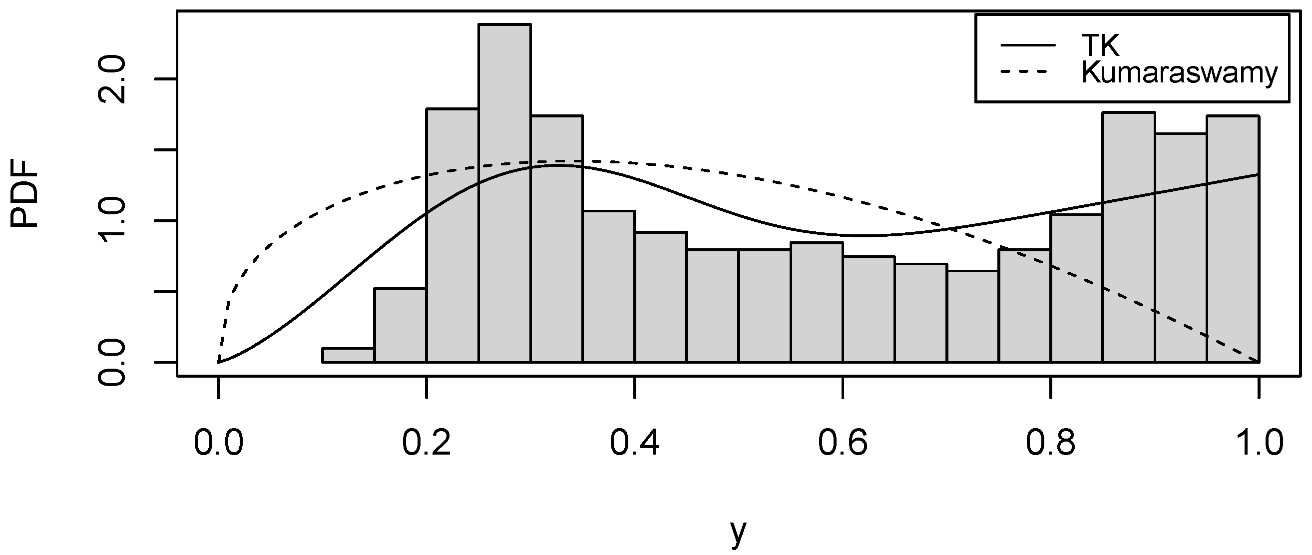
The results showed that the fit performed using the TK distribution is better than with the Kumaraswamy distribution, as there may be enough data in the tails to require a model that can describe this behavior. Note that, in Figure 3 and

Table 6. Values of the mean DIC, EAIC, and EBIC for the indicated distribution using Chilean COVID-19 data.

Distribution	Mean DIC	Mean EAIC	Mean EBIC
TK	876.3951	−207.6895	−188.9261
Kumaraswamy	424.0051	428.0051	437.3868

, the TK distribution achieves a better fit compared to the Kumaraswamy distribution. It is clear that the empirical distribution in this dataset is lifted in the right tail, as captured by $\widehat{b}=1.3264$. Moreover, in accordance with the mean EAIC and EBIC, we can conclude that the TK distribution is a much better choice for modeling these COVID-19 data.

Table 7. Estimated means, medians, and CIs for the indicated distribution using COVID-19 data.

Distribution	Parameter	Mean	Standard Deviation	Median	95% CI
TK	a	0.0009	0.0030	0	(0, 0.0050)
	b	1.3264	0.0487	1.3267	(1.2373, 1.4211)
	$\alpha$	2.4929	0.5118	2.4966	(1.4474, 3.4459)
	$\beta$	12.9142	8.4907	10.7872	(1.5407, 29.9875)
Kumaraswamy	$\alpha$	1.4027	0.5590	1.2789	(0.6033, 2.4522)
	$\beta$	2.0127	7.5916	0.8599	(0.4080, 2.1823)

presents the means, standard deviations, medians, and CIs for each model. It can be seen that $\widehat{\beta }$ has a high standard deviation compared to the mean in both models, and is less in the TK distribution. This might be explained by the higher amount of data in the right tail causing the estimation process to encounter difficulty when assigning the value of $\beta$ in each iteration, assuming that the peak is on this side. Furthermore, the standard deviation of $\widehat{\alpha }$ is considered high compared with $\widehat{\beta }$ in the Kumaraswamy distribution.

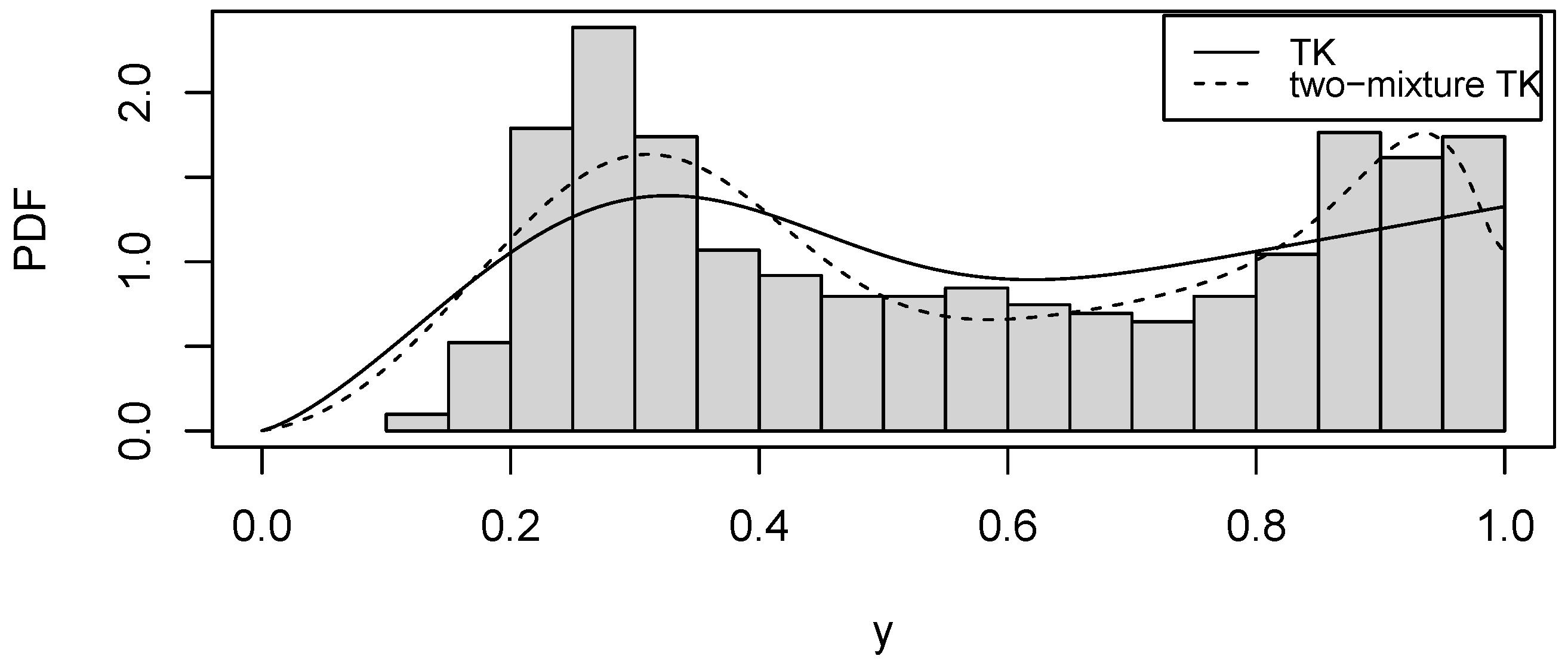
In conclusion, the TK model provides a better fit for this dataset (see Figure 4 and

Table 8. Values of the mean DIC, EAIC, and EBIC for the indicated distribution with Chilean COVID-19 data.

Distribution	Mean DIC	Mean EAIC	Mean EBIC
Two-mixture TK	−603.6924	−585.6924	−543.4748
TK	876.3951	−207.6895	−188.9261

).

Table 9. Estimated posterior means, medians, and CIs for the two-mixture TK distribution with Chilean COVID-19 data.

Parameter	Mean	Standard Deviation	Median	95% CI
$a_1$	0.0013	0.0043	0	(0, 0.0081)
$b_1$	1.6641	0.1651	1.6680	(1.3678, 2)
${\alpha }_1$	15.8136	6.8317	15.4616	(2.2682, 27.8903)
${\beta }_1$	2.9145	2.5286	2.2340	(0.0589, 8.1871)
$a_2$	0.0026	0.0097	0	(0, 0.0162)
$b_2$	0.0938	0.01952	0	(0, 0.6082)
${\alpha }_2$	3.0370	0.4966	3.065	(2.0029, 3.9354
${\beta }_2$	26.4600	15.5967	22.7700	(4.3897, 59.6894)
p	0.6120	0.0601	0.6248	(0.4671, 0.6994)

shows that the estimation of each parameter in each dataset is good when the TK distribution is adjusted. Moreover, in accordance with the mean EAIC and EBIC, we can conclude that the TK distribution is a much better choice for modeling these data.

The described situation above involving the standard deviation led us to consider whether we might be able to obtain an even better fit. This would be possible with a model based on a mixture of two TK distributions, which can be justified because this dataset is bimodal. Therefore, we could have a model using a two-mixture TK distribution defined as: $Y_i;a_j,b_j,{\alpha }_j,{\beta }_j,p_j\sim {\sum }_{j=1}^2{p}_j{f}_{\mathrm{TK}}(y;a_j,b_j,{\alpha }_j,{\beta }_j)$, for $i\in \{1,\dots ,805\}$ and $j\in \{1,2\}$, where $0<p_j\le 1$ and ${\sum }_{i=1}^2{p}_j=1$ are the weights for each individual TK distribution.

6. Concluding Remarks

The trapezoidal Kumaraswamy distribution is a new proposal derived from the Kumaraswamy distribution in the particular case of data with raised tails. This involves a generalization that allows the data in the extremes of the distribution to be fitted by adding two very intuitive new parameters. In particular, the effort of this investigation was in proposing an alternative estimation procedure based on a Bayesian approach, justified by the intuitive nature of the parameters. In addition, this proposal avoids the dependence on initial values of the usual expectation-maximization algorithm, accomplishing more reliable results. This proposal achieved very good results in both simulation and real-world data application. The trapezoidal Kumaraswamy distribution performed a better adjustment for data with some accumulation at the extremes of their distribution. In addition, by observing a real dataset consisting of Chilean COVID-19 cases, we arrived at a new proposal, that is, consideration of two trapezoidal Kumaraswamy distributions to build a mixture model. This can provide the potential benefit of performing a bimodal distribution, as shown in the application with real data. The trapezoidal Kumaraswamy mixture model achieved an even better fit than the trapezoidal Kumaraswamy model. The importance of this finding lies in the possibility of extending the model for a finite mixture of trapezoidal Kumaraswamy distributions in future work.

References

1. Kumaraswamy, P. A generalized probability density function for double-bounded random processes. J. Hydrol. 1980, 46, 79–88. [Google Scholar] [CrossRef]
2. Jones, M.C. Kumaraswamy distribution: A beta-type distribution with some tractability advantages. Stat. Methodol. 2009, 6, 70–81. [Google Scholar] [CrossRef]
3. Bayer, F.M.; Cribari-Neto, F.; Santos, J. Inflated Kumaraswamy regressions with application to water supply and sanitation in Brazil. Stat. Neerl. 2021, 75, 453–481. [Google Scholar] [CrossRef]
4. Tian, W.; Pang, L.; Tian, C.; Ning, W. Change point analysis for Kumaraswamy distribution. Mathematics 2023, 11, 553. [Google Scholar] [CrossRef]
5. Nagy, H.; Al-Omari, A.I.; Hassan, A.S.; Alomani, G.A. Improved estimation of the inverted Kumaraswamy distribution parameters based on ranked set sampling with an application to real data. Mathematics 2022, 10, 4102. [Google Scholar] [CrossRef]
6. Akinsete, A.; Famoye, F.; Lee, C. The Kumaraswamy-geometric distribution. J. Stat. Distrib. Appl. 2014, 1, 17. [Google Scholar] [CrossRef] [Green Version]
7. Akinsete, A.; Famoye, F. The beta-Pareto distribution. Statistics 2008, 42, 547–563. [Google Scholar] [CrossRef]
8. Figueroa-Zuniga, J.; Niklitschek, S.; Leiva, V.; Liu, S. Modeling heavy-tailed bounded data by the trapezoidal beta distribution with applications. REVSTAT-Stat. J. 2022, 20, 387–404. [Google Scholar]
9. Cordeiro, G.; dos Santos, B. The beta power distribution. Braz. J. Probab. Stat. 2012, 26, 88–112. [Google Scholar]
10. Cordeiro, G.; de Castro, M. A new family of generalized distributions. J. Stat. Comput. Simul. 2011, 81, 883–898. [Google Scholar] [CrossRef]
11. Cordeiro, G.; Nadarajah, S.; Ortega, E. The Kumaraswamy Gumbel distribution. Stat. Methods Appl. 2012, 21, 139–168. [Google Scholar] [CrossRef]
12. De Santana, T.; Ortega, E.; Cordeiro, G.; Silva, G. The Kumaraswamy-log-logistic distribution. J. Stat. Theory Appl. 2012, 11, 265–291. [Google Scholar]
13. Eugene, N.; Lee, C.; Famoye, F. Beta-normal distribution and its applications. Commun. Stat. Theory Methods 2002, 3, 497–512. [Google Scholar] [CrossRef]
14. Liang, Y.; Sun, D.; He, C.; Schootman, M. Modeling bounded outcome scores using the binomial-logit-normal distribution. Chil. J. Stat. 2014, 5, 3–14. [Google Scholar]
15. Nadarajah, S.; Kotz, S. The beta-Gumbel distribution. Math. Probl. Eng. 2004, 10, 323–332. [Google Scholar] [CrossRef] [Green Version]
16. Nadarajah, S.; Kotz, S. The beta exponential distribution. Reliab. Eng. Syst. Saf. 2006, 91, 689–697. [Google Scholar] [CrossRef]
17. Figueroa, J.; Sanhueza, R.; Lagos, B.; Ibacache, G. Modeling bounded data with the trapezoidal Kumaraswamy distribution and applications to education and engineering. Chil. J. Stat. 2020, 11, 163–176. [Google Scholar]
18. Cordeiro, G.; Ortega, M.; Nadarajah, S. The Kumaraswamy Weibull distribution with application to failure data. J. Frankl. Inst. 2010, 347, 1399–1429. [Google Scholar] [CrossRef]
19. Mead, M.; Abd-Eltawab, A. A Note on Kumaraswamy-Fréchet Distribution. Aust. J. Basic Appl. Sci. 2014, 8, 294–300. [Google Scholar]
20. de Pascoa, M.; Ortega, E.; Cordeiro, G. The Kumaraswamy generalized gamma distribution with application in survival analysis. Stat. Methodol. 2011, 8, 411–433. [Google Scholar] [CrossRef]
21. García, C.B.; Pérez, J.G.; van Dorp, J.R. Modeling heavy-tailed, skewed and peaked uncertainty phenomena with bounded support. Stat. Methods Appl. 2011, 20, 463–486. [Google Scholar] [CrossRef]
22. Hahn, E.D. Mixture densities for project management activity times: A robust approach to PERT. Eur. J. Oper. Res. 2008, 188, 450–459. [Google Scholar] [CrossRef]
23. McLachlan, G.; Peel, D. Finite Mixture Models; Wiley: New York, NY, USA, 2004. [Google Scholar]
24. Dempster, A.; Laird, N.; Rubin, D. Maximum likelihood from incomplete data via the EM algorithm. J. R. Stat. Soc. B 1977, 39, 1–38. [Google Scholar]
25. Anil Meera, A.; Wisse, M. Dynamic expectation maximization algorithm for estimation of linear systems with colored noise. Entropy 2021, 23, 1306. [Google Scholar] [CrossRef] [PubMed]
26. Lucini, M.M.; Van Leeuwen, P.J.; Pulido, M. Model error estimation using the expectation maximization algorithm and a particle flow filter. SIAM/ASA J. Uncertain. Quantif. 2021, 9, 681–707. [Google Scholar] [CrossRef]
27. Han, M.; Wang, Z.; Zhang, X. An approach to data acquisition for urban building energy modeling using a gaussian mixture model and expectation-maximization algorithm. Buildings 2021, 11, 30. [Google Scholar] [CrossRef]
28. Okamura, H.; Dohi, T. Application of EM algorithm to NHPP-based software reliability assessment with generalized failure count data. Mathematics 2021, 9, 985. [Google Scholar] [CrossRef]
29. Massa, P.; Benvenuto, F. Predictive risk estimation for the expectation maximization algorithm with Poisson data. Inverse Probl. 2021, 37, 045013. [Google Scholar] [CrossRef]
30. Mahdizadeh, M.; Zamanzade, E. On estimating the area under the ROC curve in ranked set sampling. Stat. Methods Med. Res. 2022, 31, 1500–1514. [Google Scholar] [CrossRef]
31. Balakrishnan, N.; Leiva, V.; Sanhueza, A.; Vilca, F. Estimation in the Birnbaum-Saunders distribution based on scale-mixture of normals and the EM-algorithm. Stat. Oper. Res. Trans. 2009, 33, 171–192. [Google Scholar]
32. Couri, L.; Ospina, R.; da Silva, G.; Leiva, V.; Figueroa-Zuniga, J. A study on computational algorithms in the estimation of parameters for a class of beta regression models. Mathematics 2022, 10, 299. [Google Scholar] [CrossRef]
33. Marchant, C.; Leiva, V.; Cysneiros, F.J.A. A multivariate log-linear model for Birnbaum-Saunders distributions. IEEE Trans. Reliab. 2016, 65, 816–827. [Google Scholar] [CrossRef]
34. Celeux, G.; Govaert, G. A classification EM algorithm for clustering and two stochastic versions. Comput. Stat. Data Anal. 1992, 14, 315–332. [Google Scholar] [CrossRef] [Green Version]
35. Celeux, G.; Diebolt, J. The SEM algorithm: A probabilistic teacher algorithm derived from the EM algorithm for the mixture problem. Comput. Stat. Q. 1985, 2, 73–82. [Google Scholar]
36. Leiva, V.; Mazucheli, M.; Alves, B. A novel regression model for fractiles: Formulation, computational aspects, and applications to medical data. Fractal Fract. 2023, 7, 169. [Google Scholar] [CrossRef]
37. Worldometers. COVID-19 Coronavirus Pandemic. Available online: www.worldometers.info/coronavirus (accessed on 21 June 2023).
38. Mazucheli, M.; Alves, B.; Menezes, A.F.B.; Leiva, V. An overview on parametric quantile regression models and their computational implementation with applications to biomedical problems including COVID-19 data. Comput. Methods Programs Biomed. 2022, 221, 106816. [Google Scholar] [CrossRef]
39. Dong, E.; Du, H.; Gardner, L. An interactive web-based dashboard to track COVID-19 in real time. Lancet Infect. Dis. 2020, 20, 533–534. [Google Scholar] [CrossRef]
40. Chakraborty, T.; Ghosh, I. Real-time forecasts and risk assessment of novel coronavirus (COVID-19) cases: A data-driven analysis. Chaos Solitons Fractals 2020, 135, 109850. [Google Scholar] [CrossRef]
41. De la Fuente-Mella, H.; Rubilar, R.; Chahuán-Jiménez, K.; Leiva, V. Modeling COVID-19 cases statistically and evaluating their effect on the economy of countries. Mathematics 2021, 9, 1558. [Google Scholar] [CrossRef]
42. Ospina, R.; Leite, A.; Ferraz, C.; Magalhaes, A.; Leiva, V. Data-driven tools for assessing and combating COVID-19 out-breaks based on analytics and statistical methods in Brazil. Signa Vitae 2022, 18, 18–32. [Google Scholar]
43. Jerez-Lillo, N.; Álvarez, B.L.; Gutiérrez, J.M.; Figueroa-Zúñiga, J.; Leiva, V. A statistical analysis for the epidemiological surveillance of COVID-19 in Chile. Signa Vitae 2022, 18, 19–30. [Google Scholar]
44. Boselli, P.M.; Soriano, J.M. COVID-19 in Italy: Is the mortality analysis a way to estimate how the epidemic lasts? Biology 2023, 12, 584. [Google Scholar] [CrossRef]
45. Da Silva, C.C.; De Lima, C.L.; Da Silva, A.C.G.; Silva, E.L.; Marques, G.S.; De Araújo, L.J.B.; De Santana, M.A. COVID-19 dynamic monitoring and real-time spatio-temporal forecasting. Front. Public Health 2021, 9, 641253. [Google Scholar] [CrossRef]
46. Sardar, I.; Akbar, M.A.; Leiva, V.; Alsanad, A.; Mishra, P. Machine learning and automatic ARIMA/Prophet models-based forecasting of COVID-19, Methodology, evaluation, and case study in SAARC countries. Stoch. Environ. Res. Risk Assess. 2022, 37, 345–359. [Google Scholar] [CrossRef]
47. Heredia Cacha, I.; Sáinz-Pardo Díaz, J.; Castrillo, M.; García, Á.L. Forecasting COVID-19 spreading through an ensemble of classical and machine learning models: Spain’s case study. Sci. Rep. 2023, 13, 6750. [Google Scholar] [CrossRef]
48. Gondim, J.A.M. Preventing epidemics by wearing masks: An application to COVID-19. Chaos Solitons Fractals 2021, 143, 110599. [Google Scholar] [CrossRef] [PubMed]
49. Vasconcelos, G.L.; Brum, A.A.; Almeida, F.A.G.; Macêdo, A.M.S.; Duarte-Filho, G.C.; Ospina, R. Standard and Anomalous Waves of COVID-19, A Multiple-Wave Growth Model for Epidemics. Braz. J. Phys. 2021, 51, 1867–1883. [Google Scholar] [CrossRef]
50. Vasconcelos, G.L.; Macêdo, A.M.S.; Duarte-Filho, G.C.; Brum, A.A.; Ospina, R.; Almeida, F.A.G. Power law behaviour in the saturation regime of fatality curves of the COVID-19 pandemic. Sci. Rep. 2021, 11, 4619. [Google Scholar] [CrossRef] [PubMed]
51. Wu, K.; Darcet, D.; Wang, Q.; Sornette, D. Generalized logistic growth modeling of the COVID-19 outbreak: Comparing the dynamics in provinces in China and in the rest of the world. Nonlinear Dyn. 2020, 101, 1561–1581. [Google Scholar] [CrossRef]
52. Pérez-Ortega, J.; Almanza-Ortega, N.N.; Torres-Poveda, K.; Martínez-González, G.; Zavala-Díaz, J.C.; Pazos-Rangel, R. Application of data science for cluster analysis of COVID-19 mortality according to sociodemographic factors at municipal level in Mexico. Mathematics 2022, 10, 2167. [Google Scholar] [CrossRef]
53. Alkady, W.; ElBahnasy, K.; Leiva, V.; Gad, W. Classifying COVID-19 based on amino acids encoding with machine learning algorithms. Chemom. Intell. Lab. Syst. 2022, 224, 104535. [Google Scholar] [CrossRef] [PubMed]
54. De Araújo Morais, L.R.; Da Silva Gomes, G.S. Forecasting daily COVID-19 cases in the world with a hybrid ARIMA and neural network model. Appl. Soft Comput. 2022, 126, 109315. [Google Scholar] [CrossRef]
55. Yousaf, M.; Zahir, S.; Riaz, M.; Hussain, S.M.; Shah, K. Statistical analysis of forecasting COVID-19 for upcoming month in Pakistan. Chaos Solitons Fractals 2020, 138, 109926. [Google Scholar] [CrossRef] [PubMed]
56. Yang, Z.; Zeng, Z.; Wang, K.; Wong, S.; Liang, W.; Zanin, M.; Liu, P.; Cao, X.; Gao, Z.; Mai, Z.; et al. Modified SEIR and AI prediction of the epidemics trend of COVID-19 in China under public health interventions. J. Thorac. Dis. 2020, 12, 165. [Google Scholar] [CrossRef] [PubMed]
57. Martin-Barreiro, C.; Ramirez-Figueroa, J.A.; Cabezas, X.; Leiva, V.; Galindo-Villardón, M.P. Disjoint and functional principal component analysis for infected cases and deaths due to COVID-19 in South American countries with sensor-related data. Sensors 2021, 21, 4094. [Google Scholar] [CrossRef] [PubMed]
58. Chimmula, V.K.R.; Zhang, L. Time series forecasting of COVID-19 transmission in Canada using LSTM networks. Chaos Solitons Fractals 2020, 135, 109864. [Google Scholar] [CrossRef]
59. ArunKumar, K.E.; Kalaga, D.V.; Sai Kumar, C.M.; Chilkoor, G.; Kawaji, M.; Brenza, T.M. Forecasting the dynamics of cumulative COVID-19 cases (confirmed, recovered and deaths) for top-16 countries using statistical machine learning models: Auto-regressive integrated moving average (ARIMA) and seasonal auto-regressive integrated moving average (SARIMA). Appl. Soft Comput. 2021, 103, 107161. [Google Scholar] [CrossRef]
60. Verma, H.; Mandal, S.; Gupta, A. Temporal deep learning architecture for prediction of COVID-19 cases in India. Expert Syst. Appl. 2022, 195, 116611. [Google Scholar] [CrossRef]
61. R Core Team. R: A Language and Environment for Statistical Computing. R Foundation for Statistical Computing: Vienna. 2022. Available online: www.r-project.org (accessed on 21 June 2023).
62. Bouguila, Z.; Monga, E.; Ziou, D. Practical Bayesian estimation of a finite beta mixture through Gibbs sampling and its applications. Stat. Comput. 2006, 16, 215–225. [Google Scholar] [CrossRef]
63. Casella, G.; Robert, C. Introducing Monte Carlo Methods with R; Springer: New York, NY, USA, 2010. [Google Scholar]
64. Diebolt, J.; Robert, C. Estimation of finite mixture distributions through Bayesian sampling. J. R. Stat. Soc. B 1994, 56, 363–375. [Google Scholar] [CrossRef]
65. Spiegelhalter, D.; Best, N.; Carlin, B.; Van Der Linde, A. Bayesian measures of model complexity and fit. J. R. Stat. Soc. B 2002, 64, 583–639. [Google Scholar] [CrossRef] [Green Version]
66. Brooks, S.P. Discussion on the paper by Spiegelhalter, Best, Carlin, and van der Linde. J. R. Stat. Soc. B 2002, 64, 616–618. [Google Scholar]
67. Carlin, B.; Louis, T. Bayes and Empirical Bayes Methods for Data Analysis; Chapman and Hall/CRC: Boca Raton, FL, USA, 2001. [Google Scholar]
68. Smithson, M.; Verkuilen, J. A better lemon squeezer? Maximum-likelihood regression with beta-distributed dependent variables. Psychol. Methods 2006, 11, 54–71. [Google Scholar] [CrossRef] [PubMed] [Green Version]
Figure 1. Plots of TK (solid line) and Kumaraswamy (dashed line) PDFs with  ( α , β ) = ( 5 , 13 )  and different values of the parameters  ( a , b )  in TK:  ( a , b ) = ( 0.4 ; 0.4 )  (left),  ( a , b ) = ( 0.0 ; 0.7 )  (center), and  ( a , b ) = ( 0.7 ; 0.0 )  (right).
Mathematics 11 02894 g001
Figure 2. Daily Chilean COVID-19 data (left) and histogram with the applied transformation (right).
Mathematics 11 02894 g002
Figure 3. Fitting plot for the TK (solid line) and Kumaraswamy (dashed line) distributions taking the mean of the parameters and histogram with Chilean COVID-19 data.
Mathematics 11 02894 g003
Figure 4. Fitting plot for the two-mixture TK (solid line) and TK (dashed line) distributions taking the parameter mean and histogram for Chilean COVID-19 data.
Mathematics 11 02894 g004