Dynamics of Newtonian Liquids with Distinct Concentrations Due to Time-Varying Gravitational Acceleration and Triple Diffusive Convection: Weakly Non-Linear Stability of Heat and Mass Transfer

Abstract

One of the practical methods for examining the stability and dynamical behaviour of non-linear systems is weakly non-linear stability analysis. Time-varying gravitational acceleration and triple-diffusive convection play a significant role in the formation of acceleration, inducing some dynamics in the industry. With an emphasis on the natural Rayleigh–Bernard convection, more is needed on the significance of a modulated gravitational field on the heat and mass transfer due to triple convection focusing on weakly non-linear stability analysis. The Newtonian fluid layers were heated, salted and saturated from below, causing the bottom plate’s temperature and concentration to be greater than the top plate’s. In this study, the acceleration due to gravity was assumed to be time-dependent and comprised of a constant gravity term and a time-dependent gravitational oscillation. More so, the amplitude of the modulated gravitational field was considered infinitesimal. The case in which the fluid layer is infinitely expanded in the x-direction and between two concurrent plates at $z=0$ and $z=d$ was considered. The asymptotic expansion technique was used to retrieve the solution of the Ginzburg–Landau differential equation (i.e., a system of non-autonomous partial differential equations) using the software MATHEMATICA 12. Decreasing the amplitude of modulation, Lewis number, Rayleigh number and frequency of modulation has no significant effect on the Nusselt number proportional to heat-transfer rates ($Nu$), Sherwood number proportional to mass transfer of solute 1 ($S{h}_1$) and Sherwood number proportional to mass transfer of solute 2 ($S{h}_2$) at the initial time. The crucial Rayleigh number rises in value in the presence of a third diffusive component. The third diffusive component is essential in delaying the onset of convection.

1. Introduction

The problem of fluid instability due to buoyancy, also known as Rayleigh–Bernard convection, is a classical problem with many real-life applications. For example, the problem where the instability occurs due to the density, which depends on two different quantities/species that diffuse in the system with different rates, is called the double-diffusive instability problem; see Turner [1]. In recent years, many researchers have explored double-diffusive convection. Antar [2] presents the influence of penetrative motion for double-diffusive convection with quadratic relation between density and temperature. Gupta et al. [3] analyzed double-diffusive convection under gravity modulation and obtained the result that the rate of mass transport decreases with the increase in Taylor number. While Bhadauria et al. [4] studied the double-diffusive Bernard–Darcy convection under temperature modulation and found that the frequency of modulation ($\omega$) and amplitude of modulation ($\delta$) has a negligible effect on the variation heat transfer for IPM (In Phase Modulation). Moreover, Siddheshwar et al. [5] studied the behaviour of the same convective system in a porous medium and showed that the influence of gravity and temperature modulation on the rate of mass and heat transport increases with an increase in solute Rayleigh number and amplitude of modulation. The double-diffusive convection problems are essential in many fields, such as electrochemistry, geophysics, solidification of two mixtures, oceanography and limnology. However, there are many situations where two solutes are present with a fluid. The convection in such a system is called triple-diffusive convection. Due to many applications, the problem of heat and mass transport in triply diffusive convective systems is now an exciting research topic. Straughan and Tracey [6] start the investigation of multi-diffusive components as applicable in the case of solute migration in water-saturated muds and chemical engineering where the chemical reaction of two reactants with fluids takes place, metallurgy in which the valuable metals are extracted from an ore chemically or physically and moisture migration via air contained in fibrous insulation. In view of this, it is important to study the dynamics of Newtonian liquids with distinct concentrations with emphasis on the heat- and mass-transfer rates.

Wollkind et al. [7] remarked on applying weakly nonlinear stability analysis for understanding the prototype reaction-diffusion. Rionero [8] obtained the condition for global nonlinear stability of the thermal conductive solution under triple-diffusive convection. Rudraiah and Vortmeyer [9] investigate the problem under the influence of permeability and reveal that the permeability minimizes the field of salt-finger and overstable modes. Tracey [10] presented the topology of the neutral curve for porous media. Further, Raghunatha [11] obtained the result for Maxwell fluid saturated porous medium and revealed that increment in relaxation parameter and the Darcy–Prandtl number enhanced the heat and mass transport rate. Moreover, Khan et al. [12] analyzed the enhancement of mass and heat transfer of the Nacl–Sucrose–water mixture for porous media and considered different types of cavities. Moreover, some researchers also explained the behaviour of triple-diffusive convection under couple stress. Shivakumara and Kumar [13] show that Oscillatory convection is possible for a value greater than one of the diffusivity ratios. Raghunatha [14] concluded that the heat and mass transfer due to the medium’s porosity decreased with increased stress parameters in the stationary case and showed the opposite nature in the oscillatory case. Moreover, Stuart [15] performed a linear stability analysis for a third diffusive component system for Maxwell fluid saturated by a porous layer under the condition of internal heat source and derived the sufficient condition of the non-existence of over stability and also showed that Lewis numbers destabilize the system. In contrast, the solute Rayleigh numbers play a stabilizing role. Although in recent times, many researchers have revealed a fascinating and essential fact about triple-diffusive convection under different situations, as mentioned above, there is also a situation where the modulation significantly affects the convection for gravity. Therefore, the influence of gravity modulation in triple-diffusive convection for a Newtonian fluid was studied. Here, the two gravity parts were assumed as the regular and time-dependent sinusoidally varying parts. Further, a weakly nonlinear theory was used to predict the variation of the rate of heat and mass transfer in terms of Nusselt number and Sherwood numbers. In this direction, it is worth noticing that the literature needs to include the study of time-varying gravitational acceleration and triple-diffusive convection of Newtonian liquids with distinct concentrations.

Finally, this theory is used to determine hydrodynamic stability. It is a method of perturbing the linear stability characteristics for disturbance of small amplitude. Systems whose behaviour cannot be effectively explained by a straightforward superposition of linear effects are referred to as “nonlinear” systems. Nonlinear systems frequently display complicated and complex dynamics, which calls for using specialist approaches to analyze them. The first steps of a nonlinear theory were taken by Stokes [16] for surface waves in deep water. Bohr [17] considered the case of capillary instability. Heisenberg [18] analyzed the instability of parallel plane flows of a viscous fluid. After applying the weakly nonlinear theory, non-dimensionalization of the parameters and analysis of the present problem were achieved using the Ginzburg–Landau equation. The Ginzburg–Landau differential equations have been used to model many physical problems. For example, regarding pattern formation, the fundamental Ginzburg–Landau differential equation (RGLE) was first obtained as a long-wave amplitude equation in the relationship with convection in binary mixtures close to the onset of instability. The complex Ginzburg–Landau differential equation (CGLE) was first derived as a modulation equation for two classical hydrodynamic stability problems, Rayleigh–Bernard convection by Newell and Whitehead [19] and Poiseuille flow by Stewartson and Stuart [20]. Multiple factors of the mathematical validity of this formal approximation scheme have been studied by Collet and Eckmann [21], Schneider [22] and van Harten [23]. In 1950, Landau and Ginzburg proposed a phenomenological theory that describes much of the behaviour seen in superconductors but is also used in convective fluid systems where phase transitions occur. The Ginzburg–Landau functional occurred in various branches of science. The name Ginzburg–Landau, of the functional and both of the equations (RGLE and CGLE), comes through a paper on superconductivity by Malashetty [24]. However, in this context, the (real, stationary) equation and the function are part of a more extensive functional system. The non-autonomous real Ginzburg–Landau Differential Equation was obtained via the analytical method. This non-autonomous real Ginzburg–Landau differential equation is solved numerically for different values of various parameters via the Runge–Kutta method with the help of the software MATHEMATICA. The various graphs are plotted for heat and mass transport using $Nu$ and $S{h}_i$ to analyze the parameters’ nature.

The research questions for studying the dynamics of Newtonian liquids with distinct concentrations due to time-varying gravitational acceleration and triple-diffusive convection with emphasis on the analysis of heat and mass transfer are

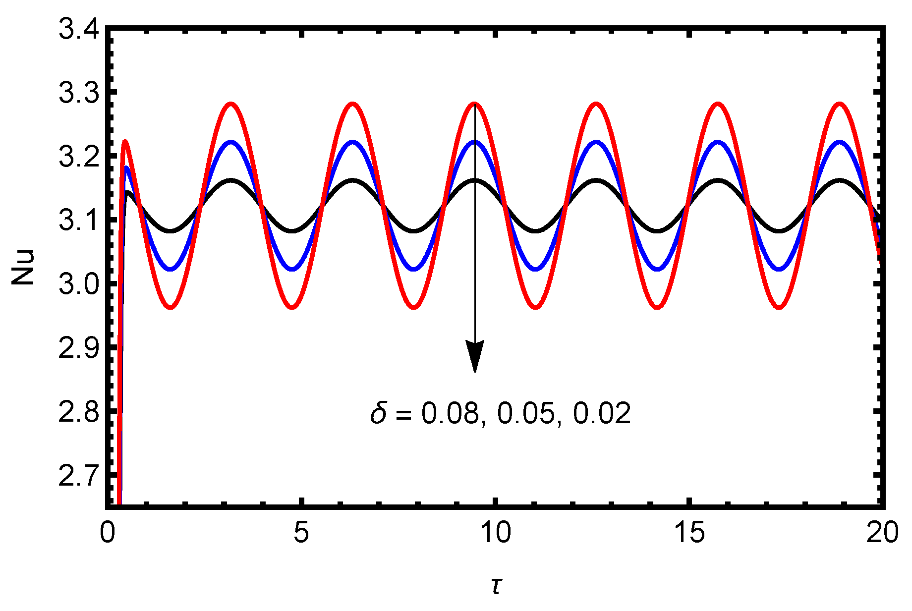
• At different levels of amplitude of modulation, how does the Nusselt number proportional to heat transfer rates ($Nu$) change with time?
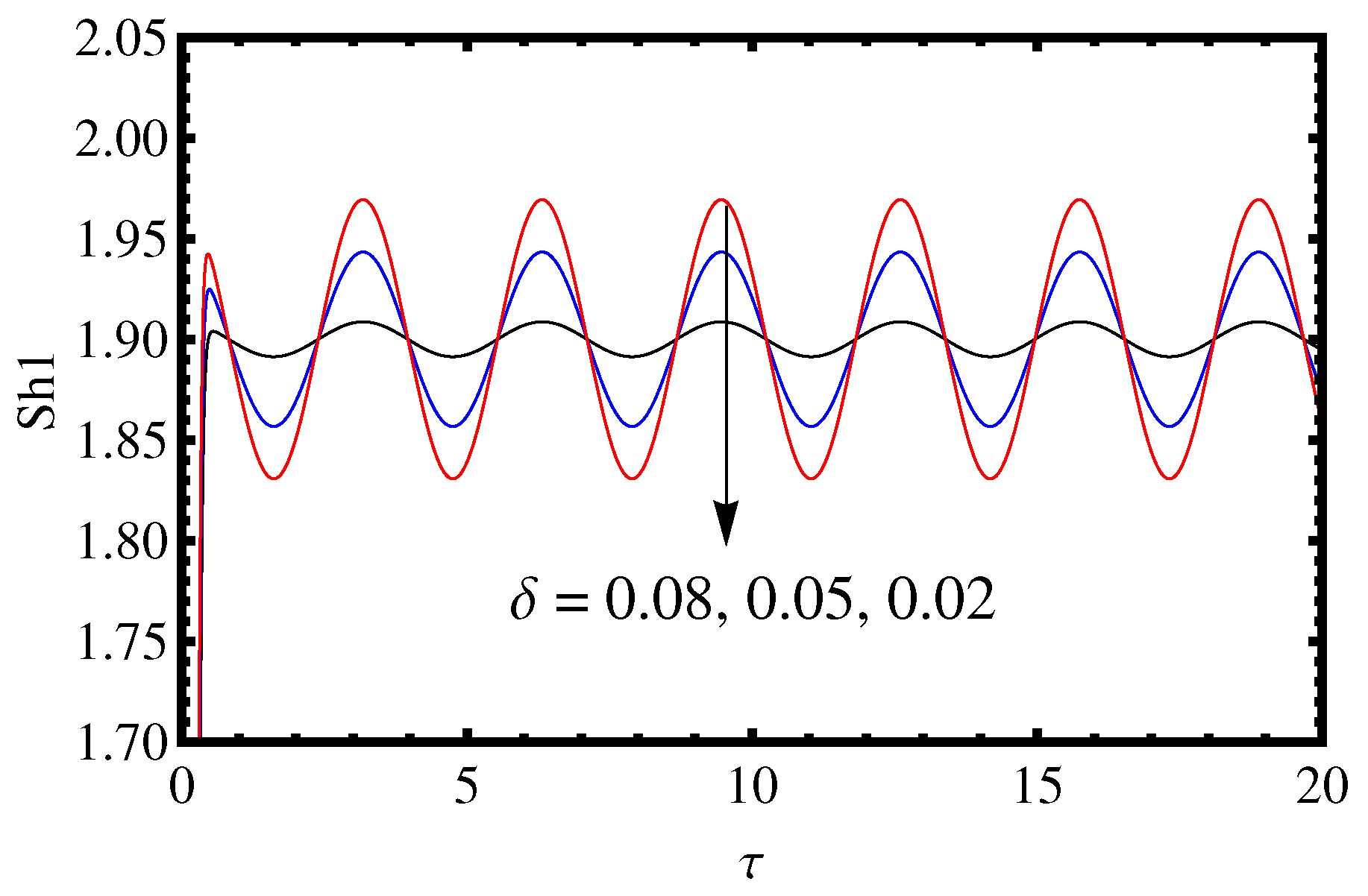
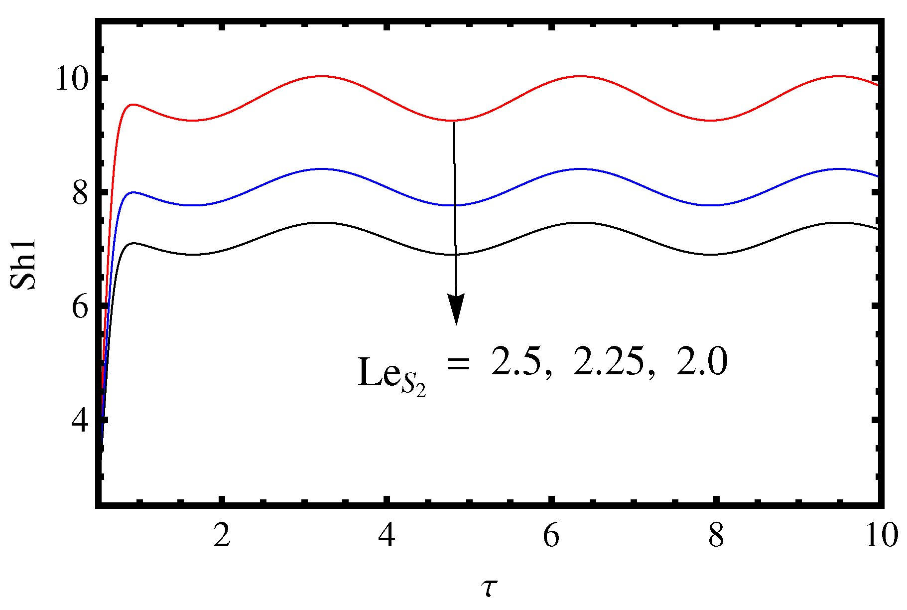
• How do decreasing Lewis number and Rayleigh number affect the Sherwood number proportional to mass transfer of solute 1 ($S{h}_1$) varying with time?
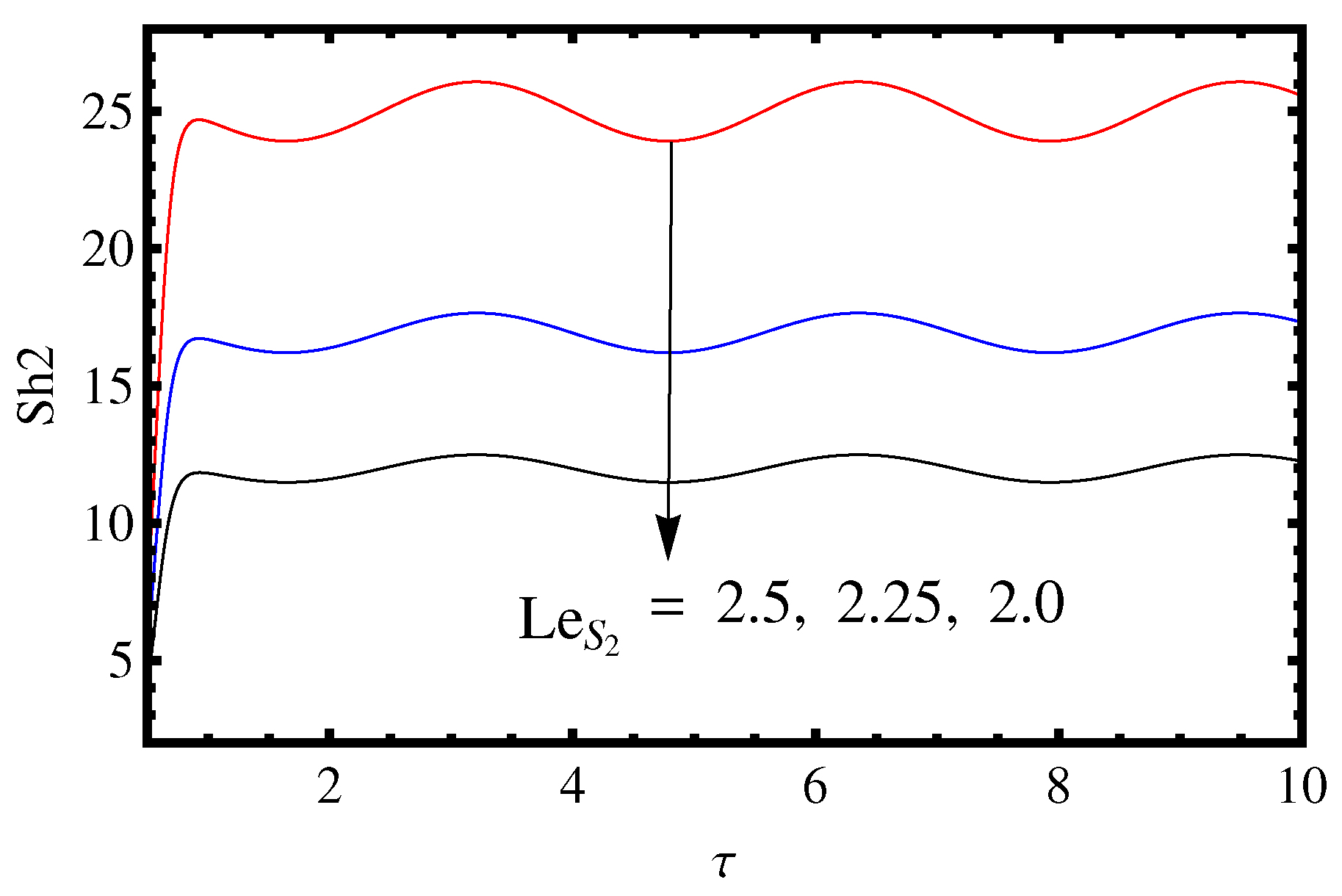
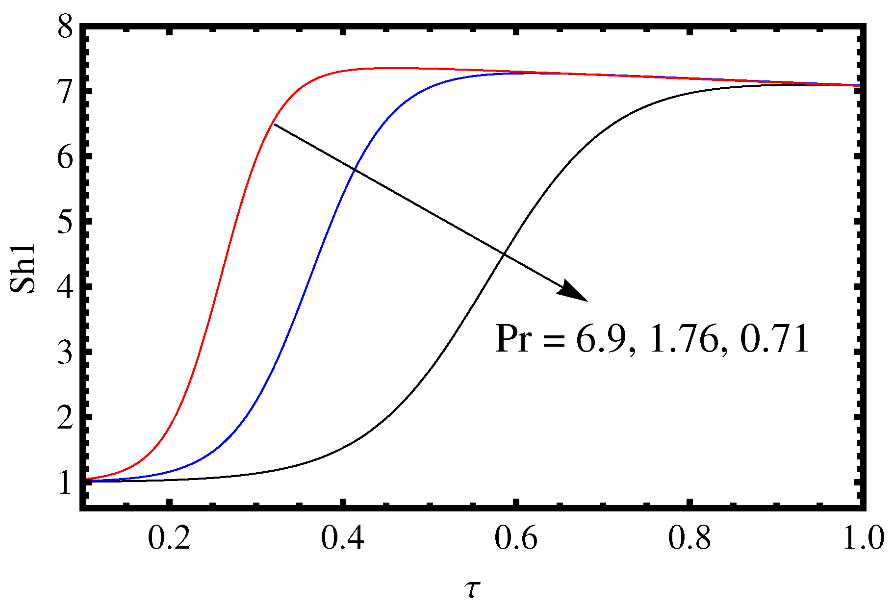
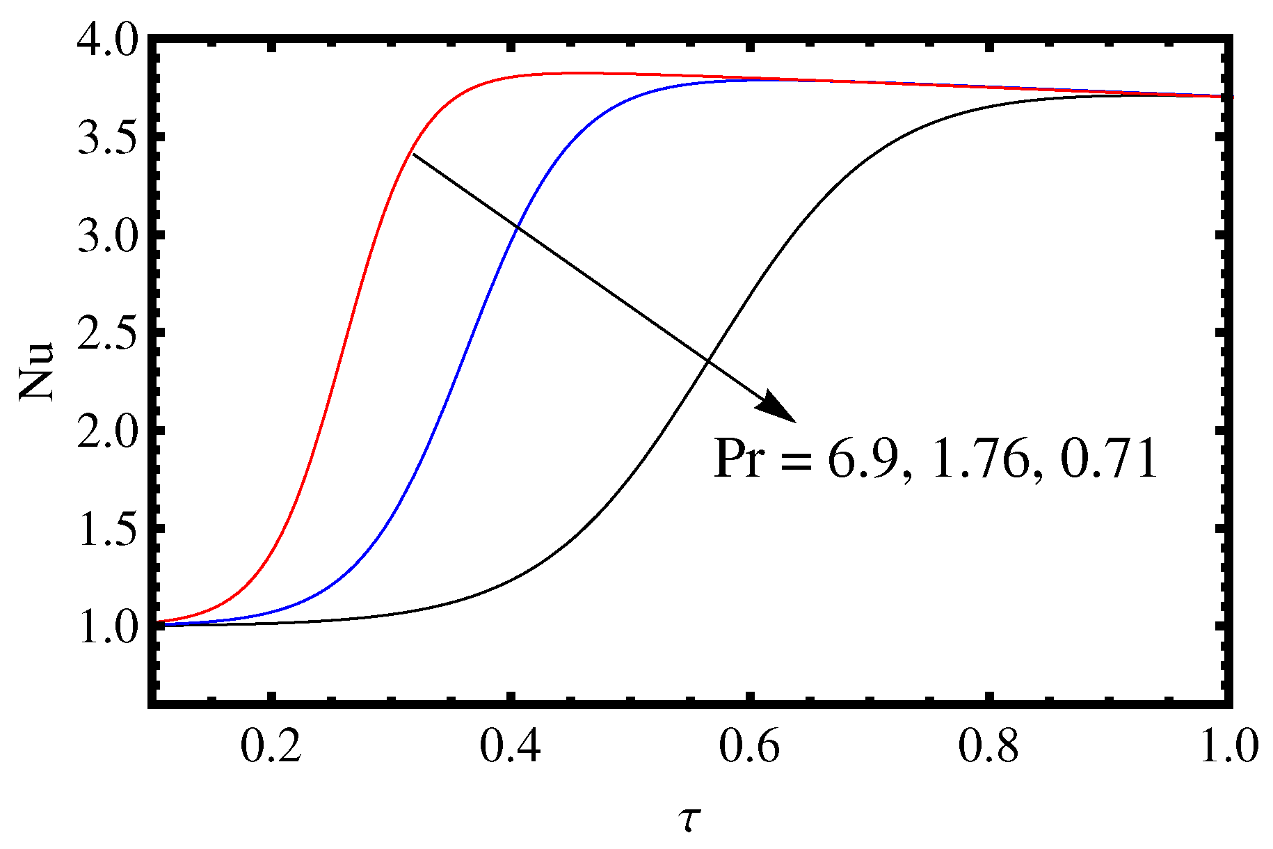
• What is the effect of decreasing Prandtl number on the Nusselt number proportional to heat transfer rates ($Nu$), Sherwood number proportional to mass transfer of solute 1 ($S{h}_1$) and Sherwood number proportional to mass transfer of solute 2 ($S{h}_2$)?

2. Research Methodology

While scientific research on gravity manipulation and other sophisticated propulsion technologies is ongoing, the practical use of gravitational modulation continues to be speculative and largely theoretical. It is a lively scientific investigation and study field, but considerable technological improvements are required to obtain such capabilities.

2.1. Formulation of the Governing Equations

As shown in Figure 1, a horizontal layer of Newtonian fluid of depth d, which includes the three components (i.e., two solutes with different concentrations and a fluid) was considered. The different values of temperature T and concentration ($S_i$) are assumed at the fluid’s bottom and top boundaries. The temperature and concentration are greater below ($z=0$) with respect to the above ($z=d$). The typical Cartesian system z-axis is vertically upward and the X- and Y-axes lie perpendicular to each other in the horizontal plane. Moreover, the system uses Boussinesq approximation, which assumes that the variation in density with temperature and solute concentration is linear and the gravity is taken as the function of t for a minimal interval time. The geometrical representation of the related problem is shown in Figure 1. The present problem is gravitational modulation with two solvents in a Newtonian fluid. Taking these assumptions, the mathematical equation of the problem is

$$\overrightarrow{g\left(t\right)}=-g_0[1+{ϵ}^2\delta cos(\Omega t)]\widehat{k}$$

(1)

where the parameters $ϵ$, $\delta$ and $\Omega$ are described in the Nomenclature section. The term $g_{{}_0}$ denotes the mean gravity (the value of $g_{{}_0}$ for space application is taken as less than or equal to ${10}^{-3}$ ms⁻²)

$$\frac{D\overrightarrow{q}}{Dt}=\frac{1}{{\rho }_0}\left[-\nabla p+\rho \overrightarrow{g\left(t\right)}+\mu {\nabla }^2\overrightarrow{q}\right],$$

(2)

$$\frac{DT}{Dt}={\kappa }_{{}_T}{\nabla }^{2}T,$$

(3)

$$\frac{D{S}_1}{Dt}={\kappa }_{S_{{}_1}}{\nabla }^2{S}_1,$$

(4)

$$\frac{D{S}_2}{Dt}={\kappa }_{S_{{}_2}}{\nabla }^2{S}_2,$$

(5)

where $D=\frac{\partial }{\partial t}+\overrightarrow{q}.\nabla$ is a substantive derivative, $\overrightarrow{q}=(u,v,w)$ is the fluid velocity, p denotes the pressure term, $\rho$ denotes the variable density of the fluid, while the solute concentrations of solute one and solute two are given by $S_1$ and $S_2$, respectively. Following Rionero [8], the Boussinesq equation is given by

$$\rho ={\rho }_{{}_0}[1-{\alpha }_{{}_T}(T-T_0)+{\beta }_{S{}_1}(S_1-S_{10})+{\beta }_{S{}_2}(S_2-S_{20})]$$

(6)

where ${\alpha }_{{}_T}$, ${\beta }_{s_{{}_1}}$ and ${\beta }_{s_{{}_2}}$ are coefficients of thermal and concentration expansion, respectively. The equation of continuity is

$$\nabla .\overrightarrow{q}=0,$$

(7)

and the boundary conditions for temperature and concentration are as follows

$$T=T_0+\Delta T\mathrm{at}z=0\mathrm{and}T=T_0\mathrm{at}z=d,$$

(8)

$$S_1=S_{10}+\Delta S_1\mathrm{at}z=0\mathrm{and}{S}_1=S_{10}\mathrm{at}z=d,$$

(9)

$$S_2=S_{20}+\Delta S_2\mathrm{at}z=0\mathrm{and}{S}_2=S_{20}\mathrm{at}z=d,$$

(10)

For the basic state of the fluid, variables are independent of time t

$$\overrightarrow{q}=\overrightarrow{q_b}=0,p=p_b\left(z\right),\rho ={\rho }_b\left(z\right),T=T_b\left(z\right),S_1=S_{1b}\left(z\right),S_2=S_{2b}\left(z\right)$$

(11)

Substituting the basic Equation (11) into Equation (6), it is worth noticing that

$$-\nabla p+{\rho }_b\overrightarrow{g\left(t\right)}=0or\frac{\partial p_b}{\partial z}={\rho }_b\overrightarrow{g\left(t\right)}$$

(12)

$$\frac{{\partial }^2{T}_b}{\partial z^2}=0$$

(13)

$$\frac{{\partial }^2{S}_{1b}}{\partial z^2}=0$$

(14)

$$\frac{{\partial }^2{S}_{2b}}{\partial z^2}=0$$

(15)

while the Boussinesq approximation becomes

$${\rho }_b={\rho }_0(1-{\alpha }_T\Delta T+{\beta }_{S1}\Delta S_1+{\beta }_{S2}\Delta S_2)$$

(16)

and the equation of continuity for the basic state is

$$\nabla .\overrightarrow{q_b}=0,$$

(17)

Taking the basic state of temperature and both solutes as a sum of the steady state and transient state leads to the equations

$$\frac{\partial T_b}{\partial z}=-\frac{\Delta T}{d},\frac{\partial S_{1b}}{\partial z}=-\frac{\Delta S_1}{d},\frac{\partial S_{2b}}{\partial z}=-\frac{\Delta S_2}{d}$$

(18)

2.2. Perturbed State and Dimensionless Variables

On applying the perturbation to the system, the perturbed variables are defined as

$$Q=Q_b+Q^{\prime }$$

(19)

where ${}^{\prime }$ defines the perturbed value and subscript b denotes basic state. Moreover, $Q=q$, p, $\rho$, T, $S_1$ and $S_2$. Now, we use the perturbed state of the system and eliminate the pressure term and then express the velocity in the form of stream function as $\overrightarrow{q^{\prime }}=(\frac{\partial \psi }{\partial z},0,-\frac{\partial \psi }{\partial x})=(u,v,z)$ for two-dimensional motion to obtain

$${\rho }_{{}_0}\left[\frac{\partial }{\partial t}\left({\nabla }^2\psi \right)-\frac{\partial (\psi ,{\nabla }^2\psi )}{\partial (x,z)}\right]={\rho }_{{}_0}{g}_{{}_0}(1+{ϵ}^2\delta cos(\Omega t))\left[-{\alpha }_{{}_T}\frac{\partial T^{\prime }}{\partial x}+{\beta }_{S{}_1}\frac{\partial S_{{}_1}^{\prime }}{\partial x}+{\beta }_{S{}_2}\frac{\partial S_{{}_2}^{\prime }}{\partial x}\right]+{\nabla }^4\psi$$

(20)

$$\frac{\partial T^{\prime }}{\partial t}-\frac{\partial (\psi ,T^{\prime })}{\partial (x,z)}-\frac{\partial T_b}{\partial x}\frac{\partial \psi }{\partial x}={\kappa }_{{}_T}\left({\nabla }^2{T}^{\prime }\right)$$

(21)

$$\frac{\partial S_{{}_1}^{\prime }}{\partial t}-\frac{\partial (\psi ,S_{{}_1}^{\prime })}{\partial (x,z)}-\frac{\partial S_{1{}_b}}{\partial x}\frac{\partial \psi }{\partial x}={\kappa }_{S{}_1}\left({\nabla }^2{S}_{{}_1}^{\prime }\right)$$

(22)

$$\frac{\partial S_{{}_2}^{\prime }}{\partial t}-\frac{\partial (\psi ,S_{{}_2}^{\prime })}{\partial (x,z)}-\frac{\partial S_{2{}_b}}{\partial x}\frac{\partial \psi }{\partial x}={\kappa }_{S{}_2}\left({\nabla }^2{S}_{{}_2}^{\prime }\right)$$

(23)

To find the dimensionless form of the variable, the redefinition of the variables below was considered

$$r=d{r}^{\ast }t=\frac{d^2}{{\kappa }_{{}_T}}{t}^{\ast },{\psi }^{\prime }={\kappa }_{{}_T}{\psi }^{\ast },(T^{\prime },T_b)=(\Delta T)(T^{\ast },T_b^{\ast })$$

(24)

$$(S_1^{\prime },S_{1b})=\left({\Delta }_1\right)(S_1^{\ast },S_{1{}_b}^{\ast }),(S_2^{\prime },S_{2{}_b})=(\Delta T)(S_2^{\ast },S_{2b}^{\ast })$$

(25)

Using the values of dimensionless parameters in Equation (20) to Equation (23), the expressions below were obtained

$$\frac{1}{P_r}\left[\frac{\partial }{\partial t^{\ast }}\left({\nabla }^2{\psi }^{\ast }\right)-J({\psi }^{\ast },{\nabla }^2{\psi }^{\ast })\right]=(1+{ϵ}^2\delta cos(\Omega t)\left[-R_{aT}\frac{\partial T^{\ast }}{\partial x^{\ast }}+R_{a{S}_1}\frac{\partial S_1^{\ast }}{\partial x^{\ast }}+R_{a{S}_2}\frac{\partial S_2^{\ast }}{\partial x^{\ast }}\right]+{\nabla }^4{\psi }^{\ast }$$

(26)

$$\frac{\partial T^{\ast }}{\partial t^{\ast }}-J({\psi }^{\ast },T^{\ast })+\frac{\partial {\psi }^{\ast }}{\partial x^{\ast }}={\nabla }^2{T}^{\ast }$$

(27)

$$\frac{\partial S_1^{\ast }}{\partial t^{\ast }}-J({\psi }^{\ast },S_1^{\ast })+\frac{\partial {\psi }^{\ast }}{\partial x^{\ast }}={\tau }_1{\nabla }^2{S}_1^{\ast }$$

(28)

$$\frac{\partial S_2^{\ast }}{\partial t^{\ast }}-J({\psi }^{\ast },S_2^{\ast })+\frac{\partial {\psi }^{\ast }}{\partial x^{\ast }}={\tau }_2{\nabla }^2{S}_2^{\ast }$$

(29)

where * denotes the dimensionless form of variables and $J(\ast ,@)=\frac{\partial (\ast ,@)}{\partial (x,z)}$ denotes the Jacobian, $P_r=\frac{\nu }{{\kappa }_{{}_T}}$ is Prandtl number, $\nu =\frac{\mu }{{\rho }_0}$ is the kinematic viscosity, $R_{a_{{}_T}}=\frac{{\alpha }_{T}g\Delta T{d}^3}{\nu {\kappa }_{{}_T}}$ is heat Rayleigh number and $R_{a_{S1}}=\frac{{\beta }_{S_1}g\Delta S_1{d}^3}{\nu {\kappa }_{{}_T}}$ and $R_{a_{S_2}}=\frac{{\beta }_{S_2}g\Delta S_2{d}^3}{\nu {\kappa }_{{}_T}}$ are solute Rayleigh number for solute one and two, respectively.

2.3. Weakly Non-Linear Stability Analysis

A complex mathematical technique used to examine the stability characteristics of dynamical systems that display nonlinear behaviour while permitting minor perturbations or deviances from equilibrium is known as weakly nonlinear stability analysis. “Weakly” means that the study concentrates on minor disruptions or deviations rather than significant departures from the equilibrium. Whether it is called weakly non-linear or weak nonlinearity, there is a strong assurance that there is only one term in the system, which is non-linear. The primary goals of weakly non-linear stability analysis are to analyse the evolution of minor perturbations to an equilibrium state and determine whether they increase, decay or remain bounded. This study, which goes beyond the linear stability analysis, which is restricted to tiny perturbations, is made possible by taking into account non-linear effects in a controlled manner. For the ingenuity of equations, the asterisk from the symbols was removed. For slow time re-scaling, the time scale such that $\tau ={ϵ}^{2}t$ then leads to Equations (26)–(29).

$$\left[{ϵ}^2\frac{dX}{d\tau }-J(\psi ,X)\right]=LX+\delta {ϵ}^{2}cos\left(\omega \tau \right)MX$$

(30)

where $J(\ast ,@)=\frac{\partial (\ast ,@)}{\partial (x,z)}$ denotes the Jacobian and the terms X, L, and M are defined as

$$X=\left[\begin{array}{c}{\nabla }^2\psi \\ T\\ S_1\\ S_2\\ \end{array}\right],L=\left[\begin{array}{cccc}{P}_r{\nabla }^2& -P_r{R}_{a_T}\frac{\partial }{\partial x}& P_r{R}_{a_{S_1}}\frac{\partial }{\partial x}& P_r{R}_{a_{S_2}}\frac{\partial }{\partial x}\\ -\frac{\partial }{\partial x}{\nabla }^{-2}& {\nabla }^2& 0& 0\\ -\frac{\partial }{\partial x}{\nabla }^{-2}& 0& {\tau }_1{\nabla }^2& 0\\ -\frac{\partial }{\partial x}{\nabla }^{-2}& 0& 0& {\tau }_2{\nabla }^2\end{array}\right]$$

(31)

$$M=\left[\begin{array}{cccc}0& -P_r{R}_{a_T}& P_r{R}_{a_{S_1}}& P_r{R}_{a_{S_2}}\\ 0& 0& 0& 0\\ 0& 0& 0& 0\\ 0& 0& 0& 0\end{array}\right]$$

(32)

Since the gravity modulation case was considered, the variables/Eigen functions of the system Equation (30) should be the function of $ϵ$ for the modulated case. Moreover, as $ϵ$ is very small with respect to executing weakly non-linear stability analysis, it is worth following the asymptotic expansion method. So, stream function $\psi$, temperature T and thermal and solute Rayleigh number $R{a}_T$, $R{a}_{S_1}$ and $R{a}_{S_2}$ are expanded in the form

$$\psi =\sum _{m=1}^{\infty }{ϵ}^m{\psi }_m,T=\sum _{m=1}^{\infty }{ϵ}^m{T}_m,$$

$$R_{aT}=\sum _{m=1}^{\infty }{ϵ}^{2m-2}{R}_{aT(2m-2)},S_1=\sum _{m=1}^{\infty }{ϵ}^m{S}_{1m},S_2=\sum _{m=1}^{\infty }{ϵ}^m{S}_{2m}.$$

(33)

Substituting Equation (33) into Equation (30) and comparing like powers of $ϵ$ up to the third degree gives the following equations.

$$L{X}_1=Y_1$$

(34)

$$L{X}_2=Y_2$$

(35)

$$L{X}_3=Y_3$$

(36)

where Equation (34) corresponds to unmodulated case and the vectors

$$Y_i=\left[\begin{array}{c}{R}_{i1}\\ R_{i2}\\ R_{i3}\\ R_{i4}\end{array}\right],X_i=\left[\begin{array}{c}{\nabla }^2{\psi }_i\\ T_i\\ S_{1i}\\ S_{2i}\end{array}\right],i=1,2,3.$$

2.3.1. First-Order Solution

Next is to find the solution at the first-order stage and obtain the minimum value of thermal Rayleigh number for the onset of convection to obtain

$$L{X}_1=Y_1$$

(37)

where the linear operator L is given as

$$L=\left[\begin{array}{cccc}{P}_r{\nabla }^2& -P_r{R}_{a_T}\frac{\partial }{\partial x}& P_r{R}_{a_{S_1}}\frac{\partial }{\partial x}& P_r{R}_{a_{S_2}}\frac{\partial }{\partial x}\\ -\frac{\partial }{\partial x}{\nabla }^{-2}& {\nabla }^2& 0& 0\\ -\frac{\partial }{\partial x}{\nabla }^{-2}& 0& {\tau }_1{\nabla }^2& 0\\ -\frac{\partial }{\partial x}{\nabla }^{-2}& 0& 0& {\tau }_2{\nabla }^2\end{array}\right]$$

(38)

and

$$X_1=\left[\begin{array}{c}{\psi }_1\\ T_1\\ S_{11}\\ S_{21}\end{array}\right]$$

(39)

It is worth knowing that the Rayleigh–Bernard convection cells are periodic. Moreover, the component of the vector $X_0$ is the time-dependent periodic function of x and z. Therefore, to find the solution of Equation (32), the next step is to assume the following time-dependent periodic solutions,

$${\psi }_1=\mathcal{A}\left(\tau \right)Sin\left(kx\right)Sin\left(\pi z\right),$$

(40)

$$T_1=\mathcal{B}\left(\tau \right)Cos\left(kx\right)Sin\left(\pi z\right),$$

(41)

$$S_{11}=\mathcal{D}\left(\tau \right)Cos\left(kx\right)Sin\left(\pi z\right),$$

(42)

$$S_{21}=\mathcal{E}\left(\tau \right)Cos\left(kx\right)Sin\left(\pi z\right),$$

(43)

and obtain the solution according to the boundary conditions

$${\psi }_1=\mathcal{A}\left(\tau \right)Sin\left(kx\right)Sin\left(\pi z\right),$$

(44)

$$T_1=-\frac{k}{p^2}\mathcal{A}\left(\tau \right)Cos\left(kx\right)Sin\left(\pi z\right),$$

(45)

$$S_{11}=-\frac{k}{p^2{\tau }_1}\mathcal{A}\left(\tau \right)Cos\left(kx\right)Sin\left(\pi z\right),$$

(46)

$$S_{21}=-\frac{k}{p^2{\tau }_2}\mathcal{A}\left(\tau \right)Cos\left(kx\right)Sin\left(\pi z\right),$$

(47)

where

$$p^2=k^2+{\pi }^2$$

(48)

Here, $\mathcal{A}\left(\tau \right)$ is undetermined and the value of $\mathcal{A}\left(\tau \right)$ will obtain at the calculation of third-order solution by using the condition of Fredholm solvability. Moreover, at this stage, it is possible to obtain the critical value of the thermal Rayleigh number ($R_a$) for the onset of convection which is given as

$$R_{a_{T_0}}=\frac{p^6}{k^2}+\frac{R{a}_{S_1}}{{\tau }_1}+\frac{R{a}_{S_2}}{{\tau }_2}$$

(49)

and the corresponding wave number is

$$and{k}_c=\frac{\pi }{\sqrt{2}}$$

(50)

The value of the critical wave number obtained here is the same as found by Chandrasekhar [25] for the classical problem of Rayleigh–Bernard convection. However, the value of the critical Rayleigh number differs by the positive sum $\frac{R{a}_{S_1}}{{\tau }_1}+\frac{R{a}_{S_2}}{{\tau }_2}$. This means that the onset of convection is a delay for the triple-diffusive convection. Moreover, from the value of the critical Rayleigh number, it is evident that the value does not depend on the amplitude of the modulation. Therefore, the onset of triple-diffusive convection is not affected by the amplitude of modulation.

2.3.2. Second-Order Solution

Next is to determine the solution at the second-order stage and the expressions of heat and mass transport in terms of Nusselt number $Nu$ and Sherwood numbers $S{h}_i$ and equate the coefficient of ${ϵ}^2$ in Equation (30) and then obtain the following equations.

$$L{X}_2=Y_2$$

(51)

where L is given by Equation (31), while $X_2$ and $Y_2$ are defined as

$$X_2=\left[\begin{array}{c}{\psi }_2\\ T_2\\ S_{12}\\ S_{22}\end{array}\right]$$

(52)

$$Y_2=\left[\begin{array}{c}{R}_{21}\\ R_{22}\\ R_{23}\\ R_{24}\end{array}\right]=\left[\begin{array}{c}0\\ \frac{\pi k^2}{2p^2}{\mathcal{A}}^2\left(\tau \right)sin\left(2\pi z\right)\\ \frac{\pi k^2}{2p^2{\tau }_1}{\mathcal{A}}^2\left(\tau \right)sin\left(2\pi z\right)\\ \frac{\pi k^2}{2p^2{\tau }_2}{\mathcal{A}}^2\left(\tau \right)sin\left(2\pi z\right)\end{array}\right]$$

(53)

In the second order, it is possible to obtain the following solutions

$${\psi }_2=0$$

(54)

$$T_2=-\frac{k^2}{8\pi p^2}{\mathcal{A}}^2\left(\tau \right)Sin\left(2\pi z\right)$$

(55)

$$S_{12}=-\frac{k^2}{8\pi {\tau }_1^2{p}^2}{\mathcal{A}}^2\left(\tau \right)Sin\left(2\pi z\right)$$

(56)

$$S_{22}=-\frac{k^2}{8\pi {\tau }_2^2{p}^2}{\mathcal{A}}^2\left(\tau \right)Sin\left(2\pi z\right)$$

(57)

The next step is to obtain the horizontally averaged Nusselt number and Sherwood numbers since

$$Nu\left(\tau \right)=\frac{[\frac{k}{2\pi }{\int }_0^{\frac{k}{2\pi }}(1+T_{{}_2}-z)dx{]}_{z=0}}{[\frac{k}{2\pi }{\int }_0^{\frac{k}{2\pi }}(1-z)dx{]}_{z=0}}$$

(58)

$$S{h}_1(\tau )=\frac{[\frac{k}{2\pi }{\int }_0^{\frac{k}{2\pi }}(1+S_{{}_{12}}-z)dx{]}_{z=0}}{[\frac{k}{2\pi }{\int }_0^{\frac{k}{2\pi }}(1-z)dx{]}_{z=0}}$$

(59)

$$S{h}_2\left(\tau \right)=\frac{[\frac{k}{2\pi }{\int }_0^{\frac{k}{2\pi }}(1+S_{{}_{22}}-z)dx{]}_{z=0}}{[\frac{k}{2\pi }{\int }_0^{\frac{k}{2\pi }}(1-z)dx{]}_{z=0}}$$

(60)

putting the values of $T_{{}_2}$, $S_{{}_{12}}$ and $S_{{}_{22}}$ from Equations (49)–(51) to obtain the following expression for Nusselt and Sherwood numbers.

$$Nu\left(\tau \right)=1+\frac{k^2}{4p^2}{\mathcal{A}}^2\left(\tau \right)$$

(61)

$$S{h}_1\left(\tau \right)=1+\frac{k^2.L{e}_{S_1}^2}{4p^2}{\mathcal{A}}^2\left(\tau \right)$$

(62)

$$S{h}_2\left(\tau \right)=1+\frac{k^2.L{e}_{S_2}^2}{4p^2}{\mathcal{A}}^2\left(\tau \right)$$

(63)

2.3.3. Third-Order Solution

To find the solution at the third-order stage and the non-autonomous Ginzburg–Landau equation, we now compare the coefficient of ${ϵ}^3$ in Equation (30) on both sides and obtain the following system of equations.

$$L{X}_3=Y_3$$

(64)

where the vector $X_3$ is given by

$$X_3=\left[\begin{array}{c}{\psi }_3\\ T_3\\ S_{13}\\ S_{23}\end{array}\right]$$

(65)

and the component of the vector $Y_3$ are

$$R_{31}=\left[-\frac{p^2}{P_r}\frac{d\mathcal{A}\left(\tau \right)}{d\tau }+\frac{k^2}{p^2}\left(R_{a_{T2}}+\delta cos\omega t\left(R_{a_{T_0}}-\frac{R_{a_{S_1}}}{{\tau }_1}-\frac{R_{a_{S_2}}}{{\tau }_2}\right)\right)\mathcal{A}\left(\tau \right)\right]sinkxsin\pi z$$

(66)

$$R_{32}=\left[-\frac{k}{p^2}\frac{d\mathcal{A}\left(\tau \right)}{d\tau }+\frac{k^3{\mathcal{A}}^3\left(\tau \right)}{4p^2}cos2\pi z\right]coskxsin\pi z$$

(67)

$$R_{33}=\left[-\frac{k}{{\tau }_1{p}^2}\frac{d\mathcal{A}\left(\tau \right)}{d\tau }+\frac{k^3{\mathcal{A}}^3\left(\tau \right)}{4{\tau }_1^2{p}^2}cos2\pi z\right]coskxsin\pi z$$

(68)

$$R_{34}=\left[-\frac{k}{{\tau }_2{p}^2}\frac{d\mathcal{A}\left(\tau \right)}{d\tau }+\frac{k^3{\mathcal{A}}^3\left(\tau \right)}{4{\tau }_2^2{p}^2}cos2\pi z\right]coskxsin\pi z.$$

(69)

Next, the Fredholm solvability condition was used to determine whether a Fredholm integral equation of the second kind has a unique solution. According to this, the time-independent part of the vector $Y_3$ must be normal to the kernel of the adjoint of the operator L. Using the expressions of $R_{31}$, $R_{32}$, $R_{33}$, and $R_{34}$ and Fredholm solvability condition for the existence of third-order solution to obtain

$$\langle Y_3,\widehat{X_1}\rangle =\underset{S}{\int \int }{Y}_3.\widehat{X_1}dS=0.$$

(70)

Firstly,  $\widehat{}$  denotes the adjoint. Secondly, $\langle ,\rangle$ defined the inner product. Thirdly, $S=[0,\frac{2\pi }{k_c}]$ X $[0,1]$. Also, $Y_3$ and $\widehat{X_1}$ are given by

$$X_1=\left[\begin{array}{c}\widehat{{\psi }_1}\\ \widehat{T_1}\\ \widehat{S_{11}}\\ \widehat{S_{21}}\end{array}\right]and{Y}_3=\left[\begin{array}{c}{R}_{31}\\ R_{32}\\ R_{33}\\ R_{34}\end{array}\right]$$

With Equation (66) and the value of $\widehat{X_1}$ and $Y_3$, to obtain the equation

$${\int }_{z=0}^{z=1}{\int }_{x=0}^{x=\frac{2\pi }{k}}[\widehat{{\psi }_1}{R}_{31}+A\widehat{T_1}{R}_{32}+B\widehat{S_{11}}{R}_{33}+C\widehat{S_{21}}{R}_{34}]dxdz=0$$

(71)

The constants A, B and C were chosen in such a way that the operator L is self adjoint after solving the above Equation (71) to obtain the values $A=1$, $B=R_{a_{T_0}}$, $C=-R_{a_{S_{11}}}$, $D=-R_{a_{S_{21}}}$ and the Ginzburg–Landau Equation of the form

$$\begin{array}{c}\left(\frac{p^2}{P_r}+\frac{k^2{R}_{a_{T_0}}}{p^4}-\frac{R_{a_{S_{11}}}{k}^2}{{{\tau }_1}^2{p}^4}-\frac{R_{a_{S_{21}}}{k}^2}{{\tau }_2^2{p}^4}\right)\frac{d\mathcal{A}\left(\tau \right)}{d\tau }=\frac{k^2}{p^2}\left(R_{a_{T_2}}+\left(R_{a_{T_0}}-\frac{R_{a_{S_1}}}{{\tau }_1}-\frac{R_{a_{S_2}}}{{\tau }_2}\right)\delta cos\Omega t\right)\mathcal{A}\left(\tau \right)\\ +\frac{k^4}{8p^4}\left[-R_{a_{T_0}}+\frac{R_{a_{S_1}}}{{\tau }_1^3}+\frac{R_{a_{S_2}}}{{\tau }_2^3}\right]{\mathcal{A}}^3\left(\tau \right)\end{array}$$

(72)

The above Ginzburg–Landau equation was solved using RK4 (Runge–Kutta fourth-order) method with initial condition $A\left(0\right)=a_0$, where $a_0$ is the amplitude of the convection at the initial stage. Moreover, it is possible to assume that $R_{{}_{T_2}}=R_{{}_{T_0}}$ to minimize the parameters.

3. Analysis of Results and Discussion

Weakly nonlinear stability analysis has a complicated meaning since it may identify elaborate patterns and behaviours that result from the interaction of nonlinear dynamics with minor disturbances. It sheds light on the presence and stability of several coherent structures that may develop in nonlinear systems, including patterns, waves and solitons. Additionally, using weakly nonlinear analysis, bifurcations—critical regions where a system’s stability characteristics undergo qualitative changes—can be found. In a concise form, we predicted the critical value of thermal Rayleigh number for the onset of the convection and impact of time-periodic modulated gravitational field (g-jitter effect) and the role of the third diffusive component on the variation of heat and mass transports in the Newtonian fluid layer. The study emphasizes the minimum value of the Rayleigh number, the heat transfer rate and the mass transfer rate. The value of the critical thermal Rayleigh number is obtained using linear stability analysis. It is worth noticing that the linear stability analysis needs to be more robust to describe the nature of the rate of heat transport. Therefore, it is possible to perform a weakly non-linear stability theory to obtain the heat and mass transfer expression in terms of Nusselt number $Nu$ and Sherwood numbers $S{h}_i$ for $i=1$ and 2.

The next step is to present the effect of non-dimensional parameters $\delta$, $L{e}_{S_1}$, $L{e}_{S_2}$, $R_{a_{S_1}}$, $R_{a_{S_2}}$ and $P_r$ on the heat and mass transport under the impact of the modulated gravitational field where the order of modulation is assumed to be very small and considered of order $O\left({ϵ}^2\right)$. As the impact of gravity modulation occurred for a concise period in the real situation, the magnitude of modulation of amplitude $\delta$ is also considered very small. For the real-life application, the range of amplitude of modulation is ${10}^{-2}<\delta <{10}^{-2}$ [26]. Moreover, for the present analysis, the frequency of modulation $\omega$ was chosen to satisfy the condition $\frac{\delta }{\omega }$≪ 1. The reason for this inequality $\frac{\delta }{\omega }$≪ 1 is explained by Venezian [27]. The parameter range was chosen in such a way that it coincides with real physical problems. The range chosen here is usually used for common fluids such as water and air. Moreover, for values of other parameters, it is worth following Bhadauria et al. [28] and assuming that $L{e}_{S_1}<L{e}_{S_2}$, $R{a}_{S_1}<R{a}_{S_2}$. Hence, in the present problem, the fixed values of dimensionless parameters as $\omega =2$, $\delta =0.05$, $L{e}_{S_1}=1.5$, $L{e}_{S_2}=2.0$, $R{a}_{S_1}=10$, $R{a}_{S_2}=20$, $P_r=0.71$ were considered. The value of minimum thermal Rayleigh number $R_{T_0}$ and the wave number $k_c$ is worth deducing from Equations (45) and (46).

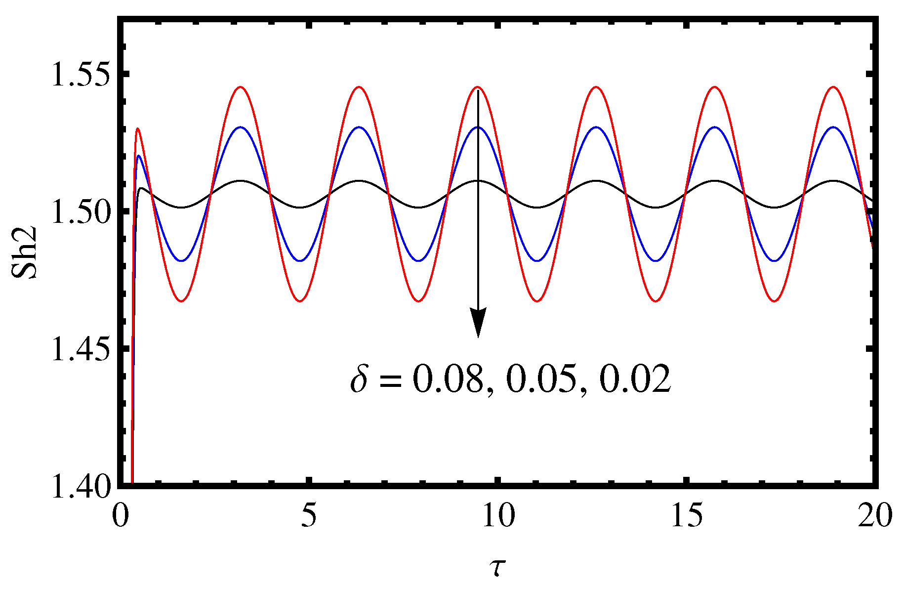
3.1. Influence of the Amplitude of Modulation

Gravitational fields are often generated by massive objects such as planets, stars or black holes and they exert an attractive effect on other things that have mass. In other words, mass diffusivity plays a significant role during amplitude of modulation. As shown in Figure 2, Figure 3 and Figure 4, the sinusoidal nature as in the case of Nusselt number proportional to heat transfer rates ($Nu$), Sherwood number proportional to mass transfer of solute 1 ($S{h}_1$) and Sherwood number proportional to mass transfer of solute 2 ($S{h}_2$) was found to disappear as the amplitude of the modulation ($\delta$) declined but the time scale grew. The manipulation or control of gravitational fields is referred to as gravitational modulation. What gravitational modulation entails is modifying gravitational force through increment, attenuation or diversion. As seen in Figure 2, Figure 3 and Figure 4, decreasing the amplitude of modulation causes the heat and mass transfer to be oscillating in nature. In Figure 2, it is worth noticing that $Nu$ increases with amplitude of modulation $\delta$ such that $Nu{/}_{\delta =0.02}<Nu{/}_{\delta =0.05}<Nu{/}_{\delta =0.08}$. Therefore, it is worth observing that the amplitude of modulation $\delta$ has a destabilizing effect on convection. This is analogous to Bhadauria et al. [28] for double-diffusive convection, but for the ongoing study, the destabilizing rate is more as compared to double-diffusive convection.

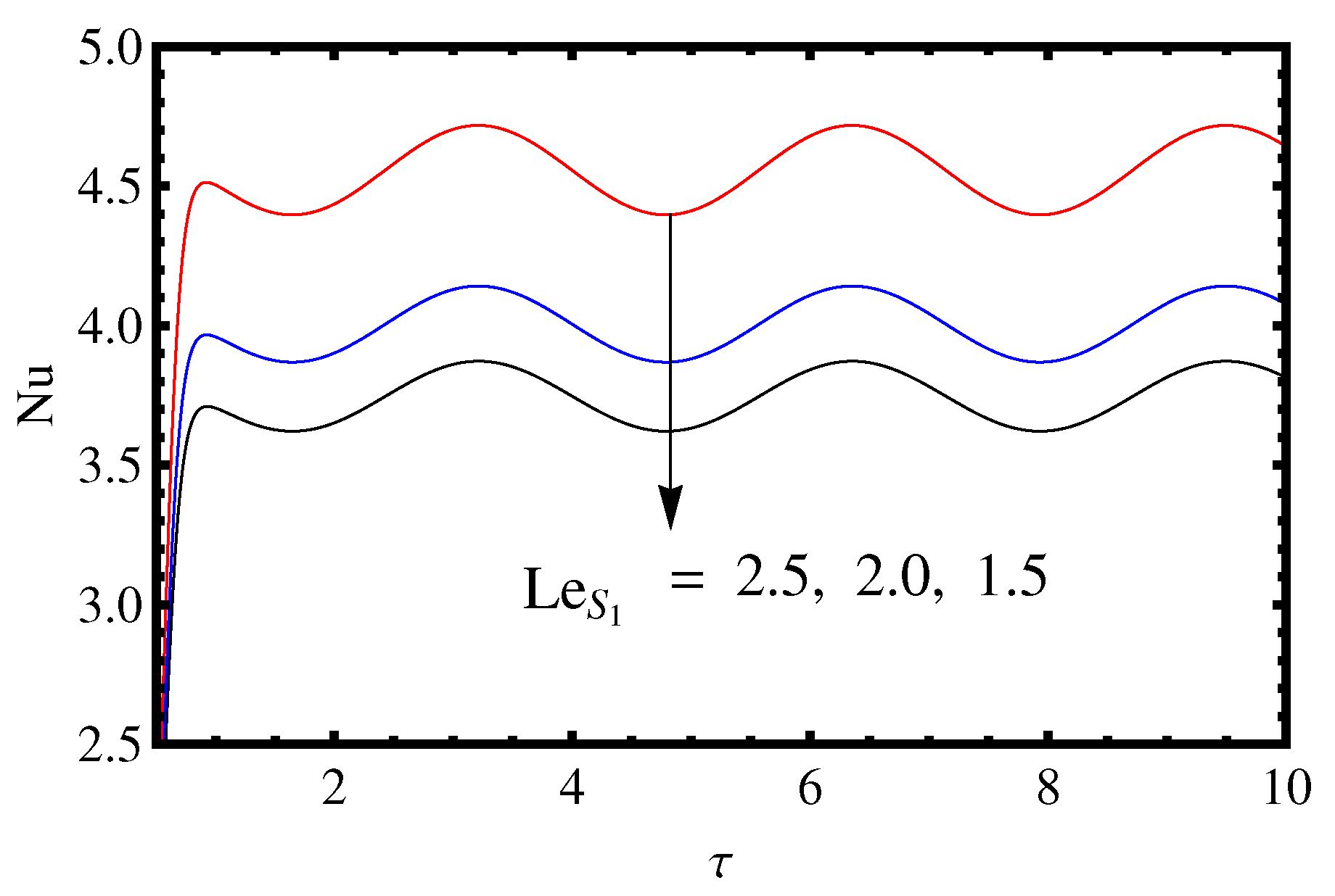
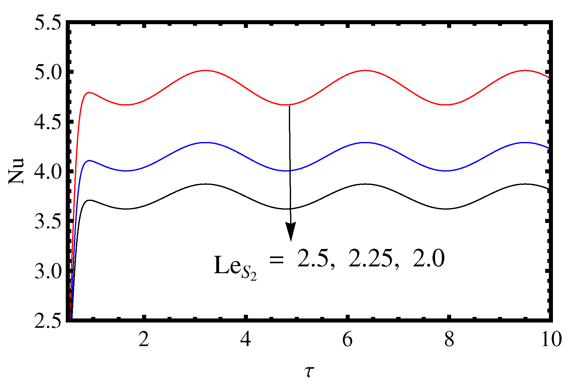
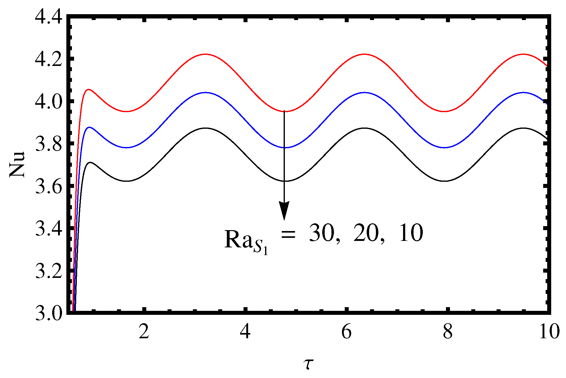
3.2. Influence of the Lewis Number and Rayleigh Number

When the Lewis number is larger than one, thermal diffusivity precedes momentum diffusivity. This is a frequent situation in gases and low-viscosity fluids. Temperature changes travel faster across the fluid in these instances than momentum transmission. Figure 5, Figure 6, Figure 7, Figure 8, Figure 9 and Figure 10 show that the Nusselt number proportional to heat transfer rates ($Nu$), Sherwood number proportional to mass transfer of solute 1 ($S{h}_1$) and Sherwood number proportional to mass transfer of solute 2 ($S{h}_2$) decline due to a lower Lewis number. The Rayleigh number gives valuable information on the behaviour of fluid flows, particularly when natural convection and heat transfer are involved. It aids in determining whether the flow is stable or unstable and it is critical in studying different natural and commercial procedures involving fluid dynamics and thermal phenomena. As seen in Figure 11, Figure 12, Figure 13, Figure 14, Figure 15 and Figure 16, the Nusselt number proportional to heat transfer rates ($Nu$), Sherwood number proportional to mass transfer of solute 1 ($S{h}_1$) and Sherwood number proportional to mass transfer of solute 2 ($S{h}_2$) decrease with lower relative importance of buoyancy forces to viscous forces in the fluid flow.

From these equations, it is clear that the critical value of the Rayleigh number is independent of the amplitude of the modulation ($\delta$). This shows that the onset of convection is not affected by the amplitude of the modulation. Moreover, the Lewis numbers and solutal Rayleigh numbers of two solutes occur in the expression of the thermal Rayleigh number, which shows that the minimum thermal Rayleigh number for triple-diffusive convection is greater than for double-diffusive convection. Thus, the presence of a third diffusive component increases the value of the minimum thermal Rayleigh number by an additional factor $\frac{R{a}_{S_1}}{{\tau }_1}$ for the onset of convection. Because the value of $\frac{R{a}_{S_1}}{{\tau }_1}$ is always positive as the ratio of two positive terms, the appearance of the third diffusing component increases the threshold value of the critical Rayleigh number. When $\omega =2$, $P_r=0.71$, $L{e}_{S_1}=1.5$, $L{e}_{S_2}=2$, $R{a}_{S_1}=10$ and $R{a}_{S_2}=20$, the variations in the Nusselt number as a yardstick for studying the heat transfer rate are presented as in Figure 2, Figure 3, Figure 4, Figure 5, Figure 6, Figure 7, Figure 8, Figure 9, Figure 10, Figure 11, Figure 12, Figure 13, Figure 14, Figure 15, Figure 16, Figure 17, Figure 18 and Figure 19. As $\delta$ decreases and $\tau \to 20$, the optimal value for $Nu\approx 3.25$, $S{h}_1\approx 1.97$ and $S{h}_2\approx 1.54$. A common Rayleigh–Bernard issue involves buoyancy-driven convection of a liquid layer heated evenly from below and contained between two parallel pure-conduction surfaces, where the tangential parts of the stress are believed to be zero; see Wollkind et al. [7].

As shown in Figure 5, Figure 6, Figure 7, Figure 8, Figure 9 and Figure 10, it is evident that the Nusselt number and mass transfer rate based on the first and second concentration diminish due to the lowering of both Lewis numbers. For a fixed thermal diffusivity, a higher Lewis number leads to a reduction in molecular diffusivity in most instances of heat and mass transfer. The Prandtl number in heat transfer is equivalent to the Schmidt number in mass transfer. The relative magnitudes of both mass and heat diffusion, mostly in thermal as well as concentration boundary layers, are represented by Lewis numbers (Animasaun et al. [29]). As $L{e}_{s2}$ decreases and $\tau \to 10$, the optimal value for $Nu\approx 4.99$ in Figure 6, $S{h}_1\approx 10$ in Figure 8 and $S{h}_2\approx 26$ in Figure 10. Figure 11, Figure 12, Figure 13, Figure 14, Figure 15 and Figure 16 depict the fact that the Nusselt number and the mass transfer rate based on the first and second concentration diminish due to a decline in both critical Rayleigh numbers. Laminar flow transitions to turbulent flow manifested at a point known as the critical Reynolds number. The Nusselt number and the mass transfer rate based on the first and second concentration rise due to the higher Prandtl number; see Figure 17, Figure 18 and Figure 19. The above results can be summarized as

$$Nu{/}_{\delta =0.02}<Nu{/}_{\delta =0.05}<Nu{/}_{\delta =0.08}$$

$$Nu{/}_{L{e}_{S_1}=1.5}<Nu{/}_{L{e}_{S_1}=2.0}<Nu{/}_{L{e}_{S_1}=2.5}$$

$$Nu{/}_{L{e}_{S_2}=2.0}<Nu{/}_{L{e}_{S_2}=2.25}<Nu{/}_{L{e}_{S_2}=2.5}$$

$$Nu{/}_{Ra{S}_1=10}<Nu{/}_{Ra{S}_1=20}<Nu{/}_{Ra{S}_1=40}$$

$$Nu{/}_{Ra{S}_2=210}<Nu{/}_{Ra{S}_2=30}<Nu{/}_{Ra{S}_2=40}$$

$S{h}_1$ and $S{h}_2$ both show effects similar to $Nu$. Meanwhile, the variations in the first Sherwood number as a yardstick for studying the mass transfer rate based on the first concentration are presented as Figure 3, Figure 4, Figure 5, Figure 6, Figure 7, Figure 8, Figure 9, Figure 10, Figure 11, Figure 12, Figure 13, Figure 14, Figure 15, Figure 16 and Figure 17. In addition, the variations in the second Sherwood number as a yardstick for studying the mass transfer rate based on the second concentration are presented as Figure 4, Figure 5, Figure 6, Figure 7, Figure 8, Figure 9, Figure 10, Figure 11, Figure 12, Figure 13, Figure 14, Figure 15, Figure 16, Figure 17 and Figure 18.

4. Concluding Remarks

Newtonian liquids’ dynamics with distinct concentrations due to time-varying gravitational acceleration and triple-diffusive convection have been examined. The impact of gravity modulation in an incompressible Newtonian liquid with a triple-diffusive component was predicted in the current research. It is believed that the fluid layers are endless, parallel and spaced apart. Ginzburg–Landau’s equation and asymptotic expansion method are applied to find the heat and mass transport rate. Based on the observations within the scope of checking the influences of different non-dimensional parameters on the convective system, it is worth concluding that:

• Decreasing the amplitude of modulation, Lewis number, Rayleigh number and frequency of modulation has no significant effect on the Nusselt number proportional to heat transfer rates ($Nu$), Sherwood number proportional to mass transfer of solute 1 ($S{h}_1$) and Sherwood number proportional to mass transfer of solute 2 ($S{h}_2$) at the initial time.
• The critical value of the thermal Rayleigh number is independent of the amplitude of the modulation ($\delta$). Thus, the onset of convection is not affected by the amplitude of the modulation.
• The crucial Rayleigh number rises in value in the presence of a third diffusive component. The third diffusive component is essential in delaying the onset of convection.
• For a small time, the amplitude of modulation increases the heat and mass transport rate and the mass transport rate is more significant than heat transport.
• The Prandtl number increases mass and heat transport for a minimal period and has a negligible effect on $Nu$, $S{h}_1$ and $S{h}_1$ after a short time interval.
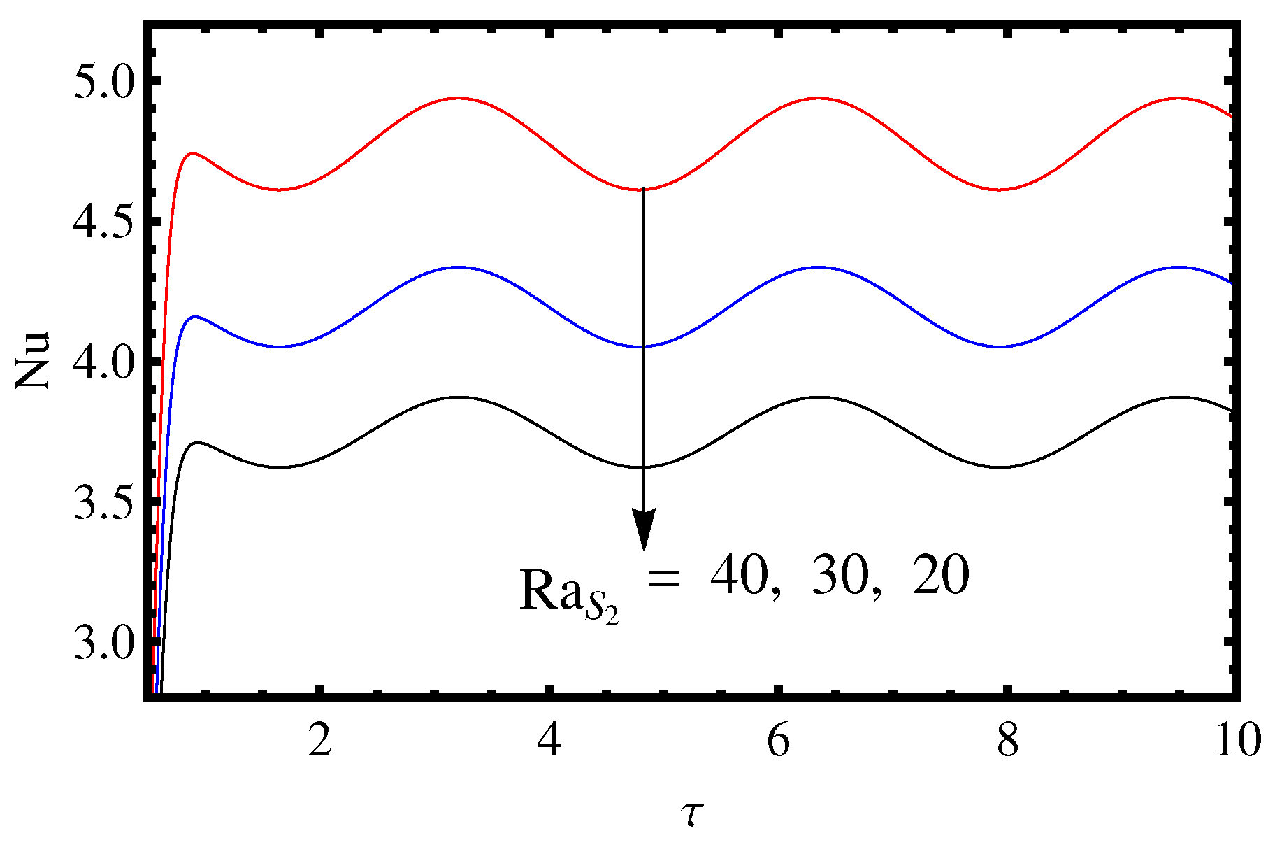
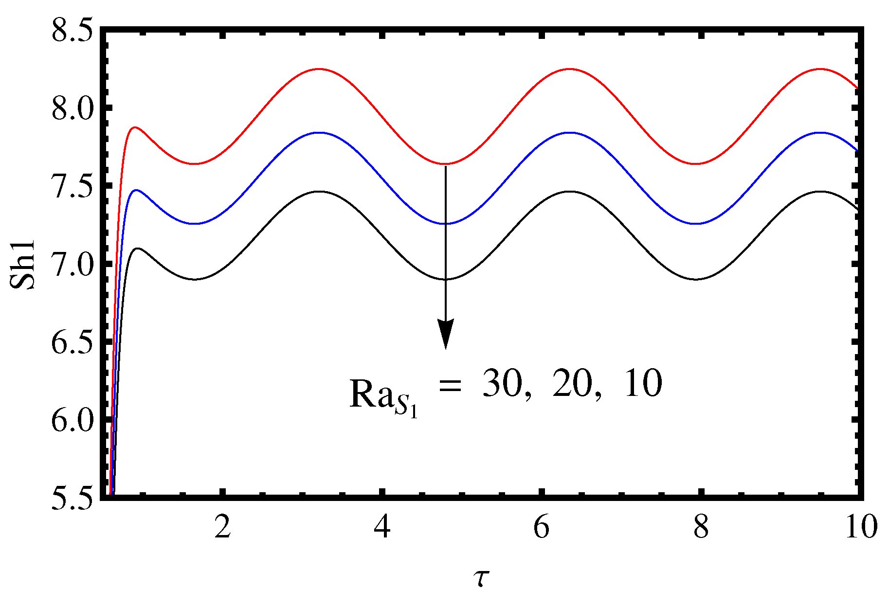
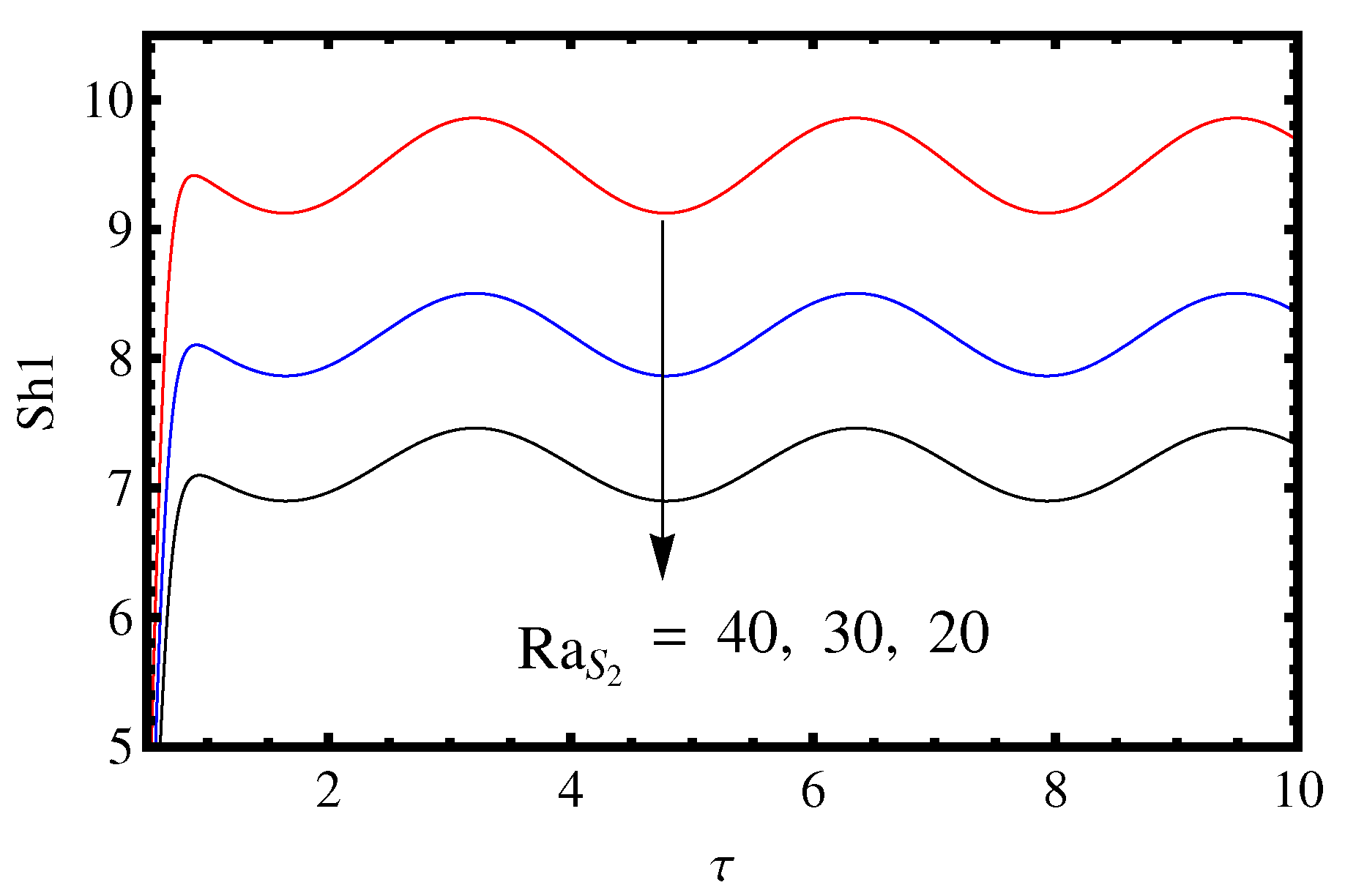
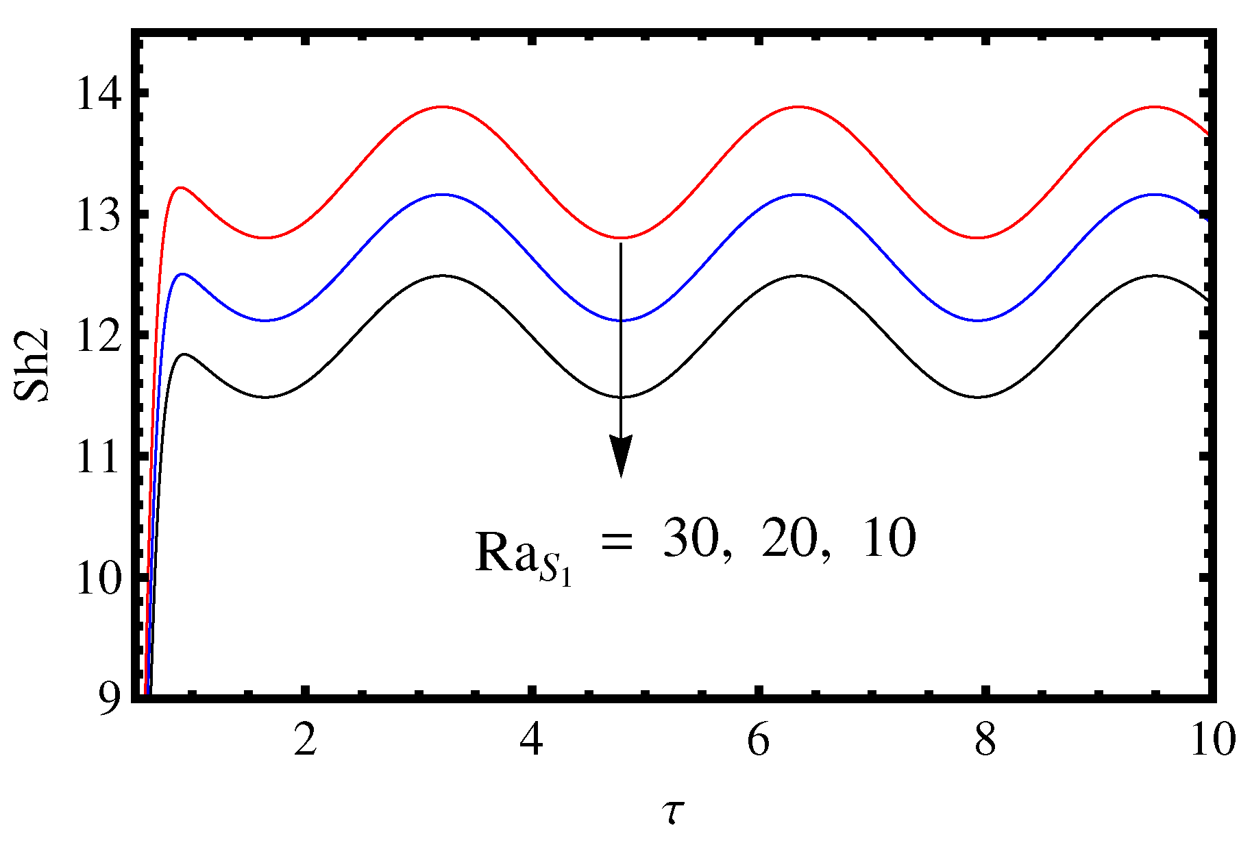
• The effect of two solute Rayleigh numbers $R{a}_{S_1}$ and $R{a}_{S_2}$ is to increase the mass and heat transport.
• The value of $Nu$, $S{h}_1$ and $S{h}_1$ decreases on increasing the value of ${\tau }_1$ and ${\tau }_2$.

Further analysis using the results by Alessa et al. [30] and Tamilvanan et al. [31] is recommended.

References

1. Turner, J.S.; Turner, J.S. Buoyancy Effects in Fluids; Cambridge University Press: Cambridge, UK, 1979; p. 251. [Google Scholar]
2. Antar, B.N. Penetrative double-diffusive convection. Phys. Fluids 1987, 30, 322–330. [Google Scholar] [CrossRef]
3. Gupta, V.K.; Kumar, A.; Singh, A.K. Analytical study of weakly non-linear mass transfer in rotating fluid layer under time-periodic concentration/gravity modulation. Int. J. Non-Linear Mech. 2017, 97, 22–29. [Google Scholar] [CrossRef]
4. Bhadauria, B.S.; Hashim, I.; Siddheshwar, P.G. Effects of time-periodic thermal boundary conditions and internal heating on heat transport in a porous medium. Transp. Porous Media 2013, 97, 185–200. [Google Scholar] [CrossRef]
5. Siddheshwar, P.G.; Bhadauria, B.S.; Srivastava, A. An analytical study of non-linear double-diffusive convection in a porous medium under temperature/gravity modulation. Transp. Porous Media 2012, 91, 585–604. [Google Scholar] [CrossRef]
6. Straughan, B.; Tracey, J. Multi-component convection-diffusion with internal heating or cooling. Acta Mech. 1999, 133, 219–238. [Google Scholar] [CrossRef]
7. Wollkind, D.J.; Manoranjan, V.S.; Zhang, L. Weakly Nonlinear Stability Analyses of Prototype Reaction-Diffusion Model Equations. SIAM Rev. 1994, 36, 176–214. [Google Scholar] [CrossRef]
8. Rionero, S. Triple-diffusive convection in porous media. Acta Mech. 2013, 224, 447–458. [Google Scholar] [CrossRef]
9. Rudraiah, N.; Vortmeyer, D. The influence of permeability and of a third diffusing component upon the onset of convection in a porous medium. Int. J. Heat Mass Transf. 1982, 25, 457–464. [Google Scholar] [CrossRef]
10. Tracey, J. Original Article Multi-component convection-diffusion in a porous medium. Contin. Mech. Thermodyn. 1996, 8, 361–381. [Google Scholar] [CrossRef]
11. Raghunatha, K.R.; Shivakumara, I.S.; Shankar, B.M. Weakly non-linear stability analysis of triple-diffusive convection in a Maxwell fluid saturated porous layer. Appl. Math. Mech. 2018, 39, 153–168. [Google Scholar] [CrossRef]
12. Khan, Z.H.; Khan, W.A.; Sheremet, M.A. Enhancement of heat and mass transfer rates through various porous cavities for triple convective-diffusive free convection. Energy 2020, 201, 117702. [Google Scholar] [CrossRef]
13. Shivakumara, I.S.; Kumar, S.N. Linear and weakly non-linear triple-diffusive convection in a couple stress fluid layer. Int. J. Heat Mass Transf. 2014, 68, 542–553. [Google Scholar] [CrossRef] [Green Version]
14. Raghunatha, K.R.; Shivakumara, I.S.; Pallavi, G. Couple stress effects on the stability of three-component convection-diffusion in a porous layer. Heat Transf. 2021, 50, 3047–3064. [Google Scholar] [CrossRef]
15. Stuart, J.T. On the non-linear mechanics of hydrodynamic stability. J. Fluid Mech. 1958, 4, 1–21. [Google Scholar] [CrossRef]
16. Stokes, G.G. On the theory of oscillatory waves. Trans. Camb. Phil. Soc. 1847, 8, 411–455. [Google Scholar]
17. Bohr, N. Determination of the surface-tension of water by the method of jet vibration. Philosophical Transactions of the Royal Society of London. Ser. A Contain. Pap. Math. Phys. Character 1909, 209, 281–317. [Google Scholar]
18. Heisenberg, W. On the stability of laminar flow. In Scientific Review Papers, Talks and Books Wissenschaftliche Ubersichtsartikel; Vortrage und Bucher; Springer: Berlin/Heidelberg, Germany, 1984; pp. 471–475. [Google Scholar]
19. Newell, A.C.; Whitehead, J.A. Finite bandwidth, finite amplitude convection. J. Fluid Mech. 1969, 38, 279–303. [Google Scholar] [CrossRef] [Green Version]
20. Stewartson, K.; Stuart, J.T. A non-linear instability theory for a wave system in plane Poiseuille flow. J. Fluid Mech. 1971, 48, 529–545. [Google Scholar] [CrossRef]
21. Collet, P.; Eckmann, J.P. The time dependent amplitude equation for the Swift-Hohenberg problem. Commun. Math. Phys. 1990, 132, 139–153. [Google Scholar] [CrossRef] [Green Version]
22. Schneider, G. Global existence via Ginzburg–Landau formalism and pseudo-orbits of Ginzburg–Landau approximations. Commun. Math. Phys. 1994, 164, 157–179. [Google Scholar] [CrossRef] [Green Version]
23. van Harten, A. On the validity of the Ginzburg–Landau equation. J. Nonlinear Sci. 1991, 1, 397–422. [Google Scholar] [CrossRef]
24. Malashetty, M.S.; Swamy, M.S. Effect of gravity modulation on the onset of thermal convection in rotating fluid and porous layer. Phys. Fluids 2011, 23, 064108. [Google Scholar] [CrossRef]
25. Chandrasekhar, S. Hydrodynamic and Hydromagnetic Stability; Oxford University Press: Oxford, UK; Dover Publications, Inc.: New York, NY, USA, 1961. [Google Scholar]
26. Wadih, M.; Roux, B. Natural convection in a long vertical cylinder under gravity modulation. J. Fluid Mech. 1988, 193, 391–415. [Google Scholar] [CrossRef]
27. Venezian, G. Effect of modulation on the onset of thermal convection. J. Fluid Mech. 1969, 35, 243–254. [Google Scholar] [CrossRef] [Green Version]
28. Bhadauria, B.S. Double diffusive convection in a porous medium with modulated temperature on the boundaries. Transp. Porous Media 2007, 70, 191–211. [Google Scholar] [CrossRef]
29. Animasaun, I.L.; Shah, N.A.; Wakif, A.; Mahanthesh, B.; Sivaraj, R.; Koriko, O.K. Ratio of Momentum Diffusivity to Thermal Diffusivity: Introduction, Meta-analysis and Scrutinization; Chapman and Hall/CRC: New York, NY, USA, 2022; ISBN-13: 978-1032108520. [Google Scholar] [CrossRef]
30. Alessa, N.; Tamilvanan, K.; Balasubramanian, G.; Loganathan, K. Stability results of the functional equation deriving from quadratic function in random normed spaces. AIMS Math. 2021, 6, 2385–2397. [Google Scholar] [CrossRef]
31. Tamilvanan, K.; Loganathan, K.; Revathi, N. HUR Stability Results of Mixed-Type Additive-Quadratic Functional Equation in Fuzzy b-Normed Spaces by Two Different Approaches. In Soft Computing Techniques in Engineering, Health, Mathematical and Social Sciences; CRC Press: Boca Raton, FL, USA, 2021; pp. 63–92. [Google Scholar]
Figure 1. Physical illustration of Phenomenon.
Mathematics 11 02907 g001
Figure 2. Effects of decreasing  δ  on  N u ( τ ) .
Mathematics 11 02907 g002
Figure 3. Effects of decreasing  δ  on  S h 1 ( τ ) .
Mathematics 11 02907 g003
Figure 4. Effects of decreasing  δ  on  S h 2 ( τ ) .
Mathematics 11 02907 g004
Figure 5. Effects of decreasing  L e S 1  on  N u ( τ ) .
Mathematics 11 02907 g005
Figure 6. Effects of decreasing  L e S 2  on  N u ( τ ) .
Mathematics 11 02907 g006
Figure 7. Effects of decreasing  L e S 1  on  S h 1 ( τ ) .
Mathematics 11 02907 g007
Figure 8. Effects of decreasing  L e S 2  on  S h 1 ( τ ) .
Mathematics 11 02907 g008
Figure 9. Effects of decreasing  L e S 1  on  S h 2 ( τ ) .
Mathematics 11 02907 g009
Figure 10. Effects of decreasing  L e S 2  on  S h 2 ( τ ) .
Mathematics 11 02907 g010
Figure 11. Effects of decreasing  R a S 1  on  N u ( τ ) .
Mathematics 11 02907 g011
Figure 12. Effects of decreasing  R a S 2  on  N u ( τ ) .
Mathematics 11 02907 g012
Figure 13. Effects of decreasing  R a S 1  on  S h 1 ( τ ) .
Mathematics 11 02907 g013
Figure 14. Effects of decreasing  R a S 2  on  S h 1 ( τ ) .
Mathematics 11 02907 g014
Figure 15. Effects of decreasing  R a S 1  on  S h 2 ( τ ) .
Mathematics 11 02907 g015
Figure 16. Effects of decreasing  R a S 2  on  S h 2 ( τ ) .
Mathematics 11 02907 g016
Figure 17. Effects of decreasing  P r  on  S h 1 ( τ ) .
Mathematics 11 02907 g017
Figure 18. Effects of decreasing  P r  on  S h 2 ( τ ) .
Mathematics 11 02907 g018
Figure 19. Effects of decreasing  P r  on  N u ( τ ) .
Mathematics 11 02907 g019
Disclaimer/Publisher’s Note: The statements, opinions and data contained in all publications are solely those of the individual author(s) and contributor(s) and not of MDPI and/or the editor(s). MDPI and/or the editor(s) disclaim responsibility for any injury to people or property resulting from any ideas, methods, instructions or products referred to in the content.